Class Notes Spring 2014

Transcription

1 Psychology 513 Quantitative Models in Psychology Class Notes Spring 2014 Robert M. McFatter University of Louisiana Lafayette Positive Emotional Intensity Extraversion Neuroticism

2 - 2 -

3 SYLLABUS Psychology Quantitative Models in Psychology Instructor: Bob McFatter Office: Girard Hall 222A; Internet page: mcfatter@louisiana.edu Texts: Kutner, M.H., Nachtsheim, C.J. & Neter, J. (2004). Applied linear regression models, fourth edition. New York: McGraw-Hill/Irwin OR Kutner, M.H., Neter, J., Nachtsheim, C.J. & Li, W. (2004). Applied linear statistical models, 5th international edition. New York: McGraw- Hill/Irwin. JMP Statistical Discovery Software, by SAS Institute. (available through UL site license at Course Description This course is designed to serve two main purposes. One objective is to provide an introduction to multiple correlation/regression and general linear models as basic analytical tools in psychological research. The other main objective is to familiarize students with a statistical package (JMP) available here and widely used throughout the country. Students should gain the practical skills necessary to enter, analyze, and interpret results for a variety of data sets using this package. The first part of the course includes an introduction to the JMP statistical package mentioned above. Students use JMP to do familiar descriptive statistics, data screening, histograms, scatterplots, t-tests, etc. A review of bivariate correlation and regression comes next if the backgrounds of the students require it. Topics covered include the relationship between correlation and regression, relevance of assumptions, effects of outliers, hypothesis testing, effects of measurement error and restricted variability, matrix formulation of regression analysis, the relation between dummy variable regression and t-test, and the interpretation of computer output including residual plots. The remainder of the course is devoted to multiple regression and closely related topics. Consideration is given to the meaning and interpretation of regression weights, part and partial correlations, enhancer and suppressor effects, stepwise regression, multicollinearity problems, polynomial, interactive and nonlinear regression, logistic regression, analysis of covariance, and the relationship between regression and analysis of variance. Two exams, a midterm and a final, are given along with numerous homework assignments involving use of the computer to illustrate the theoretical aspects of the course. Emergency Evacuation Procedures: A map of this floor is posted near the elevator marking the evacuation route and the Designated Rescue Areas. These are areas where emergency service personnel will go first to look for individuals who need assistance in exiting the building. Students who may need assistance should identify themselves to the teaching faculty

4 READING ASSIGNMENTS Sections to be covered in Kutner, M.H., Nachtsheim, C.J. & Neter, J. (2004). Applied linear regression models, fourth edition. Appendix A - Basic Results A.1, A.3-A.7 Chapter 1 - Linear Regression with One Independent Variable All sections Chapter 2 - Inferences in Regression Analysis All sections Chapter 3 - Diagnostics and Remedial Measures , 3.8 Chapter 4 - Effect of Measurement Errors 4.5 Chapter 5 - Matrix Approach to Regression Analysis All sections Chapter 6 - Multiple Regression - I , 6.9 Chapter 7 - Multiple Regression - II All sections Chapter 8 - Regression Models for Quantitative and Qualitative Predictors All sections Chapter 9 - Building the Regression Model I: Model Selection and Validation Chapter 14 - Logistic Regression, Poisson Regression, and Generalized Linear Models

5 513 NOTES OUTLINE A concise and useful review of basic statistical ideas is given in Kutner et al. s Appendix A, sections A.1, A.3-A.7. The model underlying general linear model (of which regression analysis and ANOVA are special cases) follows the general form: Data = Fit + Residual. One way this idea can be applied to the linear regression case is to describe each individual's score in the data set as being composed of 2 pieces: the predicted Y from some model, Y, and a residual or error component, e. Y Y e [1] It follows that e Y Y and reflects how far away the actual Y score is from the predicted Y score. The idea here is to hypothesize a model of the data and find estimates of the parameters of the model that make it fit the data as well as possible (i.e., minimize in some way the size of the residuals). The most common method is to find estimates of the parameters that make the sum of the squared residuals in the sample as small as possible. This is called least squares estimation. The model we focus on first is the linear regression model. The simplest case of linear regression analysis is the bivariate case: one predictor variable, X, and one criterion variable, Y. This involves fitting the sample data with a straight line of the form Y b b X 0 1 [2] where b 0 is the Y-intercept, and b 1 is the slope in the sample (these values being estimates of the population parameters 0 and 1 ). The least squares estimators, b 0 and b 1, can be shown to be as follows: b 1 r s s Y X b M b M 0 Y 1 X XY X 2 X Y n n X 2 and [3] Here r is the correlation between X and Y, s Y and s X are the standard deviations of Y and X, respectively, and M Y and M X are the means of Y and X, respectively. Example. Consider the following small data set. X Y The raw calculations may be done with X 20, Y 15, XY 49, X 94 and M X = 4 and M Y = 3, leading to Y X One way to do the JMP analysis using the Fit Y By X platform is as follows: [4] - 3 -

6 Predicted Ys and residuals are obtained by plugging values of X into the regression equation. In JMP they may be obtained by clicking the red triangle by Linear Fit and selecting Save Predicteds or Save Residuals. For values of X not in the data set, predicted values and residuals may be obtained by simply including the desired X in the data set with a missing Y value and saving predicteds and residuals. Meaning of b 0 and b 1 The parameter estimates, b 0 and b 1, are interpreted straightforwardly. The intercept b 0 is the predicted value of Y when X = 0. The slope b 1 is the predicted change in Y for a 1 unit increase in X. Standardized and Deviation Score Regression Equations The regression equation estimated above is sometimes called the raw score or unstandardized regression equation because raw scores on X plugged into the equation yield predicted raw scores on Y. If the X and Y scores are first transformed into deviation scores before computing the regression equation, the resulting equation is called the deviation score regression equation. To convert scores to deviation scores one simply subtracts the mean from each score (e.g., y = Y - M Y, and x = X - M X. I use lower case letters to indicate deviation scores). The deviation score regression equation will be of the form y b 1 x, where b 1 is exactly the same as the slope in the raw score equation. Notice that the intercept in the deviation score regression equation is zero

7 It is actually more common to transform the X and Y scores to standardized (Z) scores than to deviation scores. When this is done, the resulting equation is called the standardized regression equation. The form of the standardized regression equation is Z rz. Notice that the intercept of the standardized regression equation is zero and the slope is r, the correlation coefficient between X and Y. This equation can be obtained in JMP by right-clicking in the Parameter Estimates table and selecting Columns Std Beta. It is, unfortunately, common practice to refer to standardized regression coefficients (or weights or slopes; they all mean the same thing) as standardized betas even though the coefficients are not population parameters. One interpretation of the correlation coefficient r, then, is as the slope of the standardized regression equation. Thus, an r of.6 would mean that a 1 standard deviation increase in the value of X would lead us to predict a.6 standard deviation increase in the value of Y. The predictions made are the same regardless of which form (raw score, deviation score, standard score) of the regression equation is used. Example. Consider the following summary statistics for ACT scores and GPA. ACT GPA Mean Std Dev r 0.6 What are the predicted GPAs for individuals with ACTs of 25, 10, 27, and 20? For the raw score regression equation, b 1 =.6(.8/5) =.096, and b 0 = (20) =.68. Thus, Y X, and plugging X values into the equation gives Y X X Y Note that the standardized regression equation ( Z Y rz For X = 25, Z X = 1, Z Y. 6, Y (. 8) 308. For X = 10, Z X = -2, Z Y 12., Y (. 8) 164. For X = 27, Z X = 1.4, Z Y. 84, Y (. 8) For X = 20, Z X = 0, ZY 0, Y (. 8) 2. 6 X ) yields the same predicted Y values: - 5 -

8 One interesting and important phenomenon implied by the standardized regression equation is called regression toward the mean. Because it is always the case that 0 r 1, the predicted value of Z Y will be in absolute value than Z X, that is, generally closer to the mean of zero (in standard deviation units) than Z X. Assumptions Certain assumptions are commonly made to aid in drawing inferences in regression analysis. Those assumptions may be stated as follows: 1) The means of all the conditional distributions of Y X lie on a straight line (linearity). 2) The variances of the conditional distributions of Y X are all equal (homoscedasticity). 3) The conditional distributions of Y X are all normal. 4) The points in the sample are a random sample from the population of points. If homoscedasticity holds, then the population variance of any conditional distribution of Y X is equal to the variance of the population of residuals, and an estimate of that variance may be used as an estimate of the variance of Ys for any given X. The most commonly used estimate of the variance of the residuals is the mean square error (MSE) where MSE = Σ e 2 /(n - 2) = SSE/df E. The square root of this quantity (or Root MSE) is sometimes called the standard error of estimate for the regression analysis and would, of course, be an estimate of the standard deviation of each of the conditional distributions of Y X. It can be thought of as how far off typically one would expect actual Y values to be from the predicted Y of the regression equation. ANOVA Partitioning It is common to construct an ANOVA partitioning of the variation (SS) of the Y scores in a regression analysis. 2 The total variation of the raw Y scores is measured by SSY or SSTO = ( Y MY ) y 2. The variation of the predicted Y scores is SSR = ( 2 Y M ) y Y 2. The variation of the residuals is SSE = ( Y Y ) 2 e It is straightforward to show that SSTO = SSR + SSE. This is another example of the Data = Fit + Residual idea. The total variation of the Y scores can be broken down into two pieces: (1) predictable variation due to the model (SSR); and (2) unpredictable, noise, or error variation (SSE). It also turns out that the proportion of variation in Y that is predictable is equal to r 2 : 2 2 SSR rxy ryy. [5] SSTO Sums of squares (SS) are converted into sample variance estimates or mean squares (MS) by dividing by the appropriate df. For the ANOVA breakdown here, df TO = n - 1, df R = 1, and df E = n - 2, so that MSTO = SSTO/df TO, MSR = SSR/df R, and MSE = SSE/df E. MSTO would thus be simply the sample variance of the Y scores, and MSE would be the sample variance of the residuals using n - 2 as the df. The overall F-ratio from the ANOVA breakdown, F(df R, df E ) = MS R /MS E, tests the null hypothesis that none of the variation in Y is linearly predictable from X. In the bivariate case this is exactly equivalent to the null hypothesis that the population slope, β 1, is equal to zero

9 Example. The following hypothetical predictive validity regression analysis will illustrate the ideas in this and the following sections. Test score is the X variable and Job performance is the criterion. Test Score Job Perf Bivariate Fit of Job Perf By Test Score Job Perf Test Score Linear Fit Linear Fit Job Perf = Test Score Summary of Fit RSquare RSquare Adj Root Mean Square Error Mean of Response 376 Observations (or Sum Wgts)

10 Analysis of Variance Model Error Prob > F C. Total Parameter Estimates Term Estimate Std Error t Ratio Prob> t Lower 95% Upper 95% Std Beta Intercept Test Score Test Score Job Perf Pred Formula Job Perf Residual Job Perf PredSE Job Perf StdErr Indiv Job Perf Studentized Resid Job Perf Sampling Distributions of b 0 and b 1 Because b 0 and b 1 are sample statistics, their values will fluctuate from sample to sample from the same population of X and Y values. It is common to assume a model to describe the population of X and Y values, and consider b 0 and b 1 to be estimates of the parameters of the model. The most commonly assumed model is the normal error regression model: Y i = β 0 + β 1 X i + ε i [6] where: Y i is the observed value of the criterion variable for the ith observation X i is a known constant, the value of the predictor variable for the ith observation β 0 and β 1 are parameters the residuals, ε i, are independent and N(0, σ 2 ) i = 1,..., n [i.e., normally distributed with mean 0 and variance σ 2 ] Thus, b 0 and b 1 are estimates of β 0 and β 1, and will, like all statistics, have sampling distributions associated with them. Under the normal error regression model above, the sampling distributions of b 0 and b 1 will both be normal. The means of the sampling distributions will be E{b 0 } = β 0 and E{b 1 } = β 1, respectively. Thus, b 0 and b 1 are both unbiased estimators of their respective population parameters. The variances of the two sampling distributions may be shown to be: M X For b 0 : { b0} 2. [7] n ( X i M X ) - 8 -

11 For b 1 : 2 2 { b1}. [8] 2 ( X M ) i X Sample estimates of these variances may be obtained by replacing σ 2 with its sample estimate, the mean square error (MSE). Thus, M X s { b0} MSE n 2 and [9] ( X i M X ) s 2 { b } MSE ( X M ) 1 2 i X. [10] The square roots of these quantities are called the standard errors of the parameter estimates and are given by most regression programs (including JMP) in a column next to the estimates themselves. The standard errors of b 0 and b 1 reflect how far off, typically, one would expect the sample values, b 0 and b 1, to be from β 0 and β 1, respectively. The standard errors of b 0 and b 1 can be used to construct confidence intervals around b 0 and b 1 and to conduct hypothesis tests about β 0 and β 1. To avoid the somewhat cumbersome curly brace notation, I will generally use s b0 and s b1 to refer to the standard errors of b 0 and b 1. In the predictive validity example above, s b0 = and s b1 = Hypothesis Tests and Confidence Intervals for β 1, β 0, and ρ It is common to test hypotheses and construct confidence intervals for β 1, β 0 and ρ where ρ is the population correlation between X and Y. Because 1 Y, [11] X it is clear that β 1 = 0 when ρ = 0, and vice versa. Therefore, testing the null hypothesis that either of these is equal to zero is exactly equivalent to testing the hypothesis that the other is zero. These equivalent hypotheses are the most commonly tested null hypotheses in bivariate regression analyses because they test whether there is a relation between X and Y, often the hypothesis of most interest in the analysis. When the sampling distribution of a statistic is normal, and the standard deviation of the sampling distribution of that statistic (i.e., the standard error of the statistic) can be estimated, a t-test may be constructed to test null hypotheses about the value of the population parameter the statistic estimates. The general form of the t-test is Statistic Hypothesized value t. [12] Estimated Std Error of the Statistic Thus, to test H 0 : β 1 = 0, the appropriate t-test is t b1 0 b 1. s s b1 b1-9 -

12 In the example above, t(11) = / = 4.82, p =.0005, and the H 0 : β 1 = 0, would be rejected even at α =.001. The estimated standard error of r when ρ = 0 is s with t r s r r 2 1 r, so testing the H 0: ρ = 0 can be carried out n 2 r n 2. The df associated with the t-tests for these two null hypotheses are n r Because the two t-tests are testing equivalent null hypotheses, the values of t obtained in the two tests will be exactly the same. It is also important to note that the overall F-ratio from the bivariate regression analysis described above, F(df R, df E ) = F(1, n - 2)= MS R /MS E, is exactly equivalent to the square of the t value obtained testing the null hypotheses β 1 = 0 or ρ = 0. So, these three hypothesis tests all test the same basic question and will all have exactly the same p-level. In the example above, r = , and plugging this value into the equation above yields t(11) = 4.82, p = Also, F(1, 11) = 23.23, p = Note that = b Similar logic yields a test of H 0 : β 0 = 0 of the form t 0, but this hypothesis is usually not of as much interest as the ones described above. JMP provides values for all the crucial components of these hypothesis tests including t values, F-ratio, and p-levels. In addition, confidence intervals around b 0 and b 1 may be obtained in the usual way. For example, the 1 - α confidence limits for β 1 would be b 1 ± t(1 - α/2, n - 2) s b1. In JMP the 95% confidence limits for β 0 and β 1 may be obtained by right-clicking on the Parameter Estimates table and selecting Columns Lower 95% and Upper 95%. In the example above, the 95% confidence interval for β 1 would be (from the output): (3.38, 9.05). Confidence intervals around r may be obtained using the Fisher s Z r transformation: Z r = tanh -1 (r) = 1 1 r ln. Fisher s Z r values are approximately normally distributed with a standard 2 1 r deviation of Zr s b 0 1. Ordinary normal distribution methods can thus be used to find confidence n 3 intervals around the Z r values. The ends of the confidence interval obtained may then be transformed back to r values using r = tanh( Z r ). [See p in Kutner et al. or an introductory statistics text such as HyperStat Online ( for more details and examples.] Two Kinds of Prediction (E{Y X} and Y X) [See p. 52 and 55 in Kutner et al.] There are two kinds of prediction that one might consider following a regression analysis: 1) prediction of the mean value of Y for all observations with a given X score (i.e., E{Y X}); 2) prediction of the value of Y for an individual observation with a given X score (i.e., Y X). It is important to recognize that the predicted value of Y will be the same for both cases, namely, Y. However, the uncertainty associated with the two kinds of prediction will differ

13 In the first case we are trying to predict the Y value of the population regression line for the given X, and the uncertainty associated with that prediction will be simply how far typically we would expect sample regression lines to wobble in the Y direction around the population regression line. In the second case we must consider not only this wobble of sample regression lines around the population regression line, but also the variability of individual Ys around the sample regression line. Thus, the variability in the second case will simply be the variability in the first case (i.e., wobble) plus an additional component reflecting the variability of the Ys around the sample regression line. Kutner et al. show that a sample estimate of the (wobble) variance of the Y s around the population regression line is 2 2 s Y 1 X h M X h MSE, [13] n 2 X i M X where X h is the value of X for which we wish to estimate the mean Y value (i.e., Y h ). Notice that the uncertainty depends on how far away X h is away from the mean of X, M X. The further X h is from M X, the greater the uncertainty. The square root of this quantity is called the Std Error of Predicted by JMP and can be obtained for each observation from the Fit Model platform after a regression analysis has been performed by right-clicking on a section title and selecting Save Columns Std Error of Predicted. In the above example, the predicted job performance for individuals with a test score of 60 is One would expect this value to be off typically by points from the true mean performance of individuals with a score of 60 on the test. A sample estimate of the variance of the individual Ys around the sample regression line would then be the sum of the wobble variance above and the MSE. Kutner et al. call this s 2 {pred}: 2 2 X h M X s pred MSE 1 1. [14] 2 n X i M X The square root of this quantity is called Std Error of Individual by JMP and can be obtained for each observation by selecting Save Columns Std Error of Individual. In the above example, the predicted job performance for an individual with a test score of 60 is One would expect this value to be off typically by points from the actual performance of an individual with a score of 60 on the test. It is instructive to compare this interpretation with the interpretation at the end of the last paragraph. The standard errors of predicted and individual scores may be used with the t distribution in the usual way to construct confidence intervals for the two kinds of prediction. In the Fit Y by X platform of JMP, plots of the 95% confidence intervals for the two kinds of prediction may be obtained by clicking the Linear Fit red triangle and selecting Confid Curves Fit and Confid Curves Individual, respectively. (See the figure in the output for the example above.) Actual upper and lower bounds of the 95% confidence intervals for each observation may be obtained from the Fit Model platform regression analysis by right-clicking on a section title and selecting Save Columns Mean Confidence Interval or Indiv Confidence Interval, respectively. Residuals Analysis and Outliers Examining the residuals, e i, from a regression analysis is often helpful in detecting violations of the assumptions underlying the model. The least squares estimation procedure forces the residuals to sum to

14 zero and to have a zero correlation with the predictor variable X. However, important diagnostic information can often be gained by analyzing the obtained residuals in various ways. It is common, for example, to plot the residuals as a function of X or Y (the two plots would look exactly the same except for the scale of the horizontal axis make sure you see why). This kind of plot can easily reveal nonlinearity of the relation or violations of the homoscedasticity assumption. For example, the following scatterplot and residual plot illustrates violations of both the linearity and homoscedasticity assumptions. Outliers are extreme observations whose values lie far from the values of the other observations in the data. These observations can strongly affect the fitting of a model to the data. It is common practice to examine data for outliers and perhaps remove extreme observations before fitting a model. Observations that lie more than 3 or 4 standard deviations away from the mean of the other observations are usually considered outliers. In the bivariate regression case the residuals (or better, the studentized residuals, i.e., the residuals divided by their standard errors) can be helpful in identifying outliers. Observations with studentized residuals >3 or 4 would be considered outliers. JMP provides these studentized residuals from the Fit Model platform under the Save Columns menu. In multivariate situations the Multivariate platform in JMP provides an outlier analysis that uses a measure of distance (called Mahalanobis distance) of observations from the centroid of the data in multidimensional space. Again, points with distances of > 3 or 4 from the other points would be considered outliers. The presence of outliers can, of course, strongly affect the size of the obtained correlation between two variables. Other factors that can affect the size of the correlation are (1) restriction of variability in either X or Y; (2) measurement error or unreliability in the measurement of X or Y; (3) differences in the shapes of the marginal distributions of X and Y; and (4) nonlinearity of the relation between X and Y. All of these factors tend to make the correlation between X and Y smaller than would otherwise be the case. Instructive online simulation demonstrations of (1) and (2) can be found at the HyperStat Online site or directly at

15 Two-Predictor Models When there are two predictors in the model the simplest fitted regression equation becomes Y b0 b1 X1 b2 X. [15] 2 As we have seen, the simple bivariate regression equation (Equation [2]) represents the finding of the best fitting straight line to a two dimensional scatterplot of X and Y. When there are two predictors in the model, the equation in [15] represents the finding of the best fitting plane to a three dimensional cloud of points in 3-space. The Fit part of Data = Fit + Residual is now a plane rather than a straight line. By adding predictors to, or changing the functional form of predictors in, equation [15] we may generate a huge variety of models of data, but the basic principles of model fitting, estimation of parameters, and hypothesis testing remain the same. The sample statistics b 0, b 1, and b 2 in [15] are estimates of the population parameters β 0, β 1, and β 2. Formulas for the least squares estimates of the population parameters β 1 and β 2 may be found and involve the sample variances and covariances of the Xs and Y. These formulas quickly become very complex with more than two predictors, and it is generally most satisfactory to solve the least squares estimation problem in matrix form. We will consider that later. It is impractical to compute these estimates with a calculator, so we generally use a statistics program. The intercept b 0, however, will always be b 0 = M Y - b 1 M 1 - b 2 M 2... regardless of the number of predictors, where M Y is the mean of Y, M 1 the mean of X 1, etc. Example. The following example with hypothetical data from a study using IQ and Extraversion scores to predict Sale Success will illustrate the analysis. Here is the JMP output from the Fit Model platform. Raw Data IQ Extr Success Variable N Mean Std Dev Min Max Extr IQ Success Multivariate Correlations IQ Extr Success IQ Extr Success

16 Response Success Summary of Fit RSquare RSquare Adj Root Mean Square Error Mean of Response 4.7 Observations (or Sum Wgts) 10 Analysis of Variance Model Error Prob > F C. Total MODEL 1 - IQ ALONE Parameter Estimates Term Estimate Std Error t Ratio Prob> t Std Beta Intercept IQ Effect Tests Source Nparm DF Sum of Squares F Ratio Prob > F IQ Sequential (Type 1) Tests Source Nparm DF Seq SS F Ratio Prob > F IQ Response Success Summary of Fit RSquare RSquare Adj Root Mean Square Error Mean of Response 4.7 Observations (or Sum Wgts) 10 MODEL 2 - EXTR ALONE Analysis of Variance Model Error Prob > F C. Total Parameter Estimates Term Estimate Std Error t Ratio Prob> t Std Beta Intercept Extr Effect Tests Source Nparm DF Sum of Squares F Ratio Prob > F Extr Sequential (Type 1) Tests Source Nparm DF Seq SS F Ratio Prob > F Extr

17 Response Success Summary of Fit RSquare RSquare Adj Root Mean Square Error Mean of Response 4.7 Observations (or Sum Wgts) 10 MODEL 3 - IQ FIRST Analysis of Variance Model Error Prob > F C. Total Parameter Estimates Term Estimate Std Error t Ratio Prob> t Std Beta Intercept IQ Extr Effect Tests Source Nparm DF Sum of Squares F Ratio Prob > F IQ Extr Sequential (Type 1) Tests Source Nparm DF Seq SS F Ratio Prob > F IQ Extr Response Success Summary of Fit RSquare RSquare Adj Root Mean Square Error Mean of Response 4.7 Observations (or Sum Wgts) 10 MODEL 4 - EXTR FIRST Analysis of Variance Model Error Prob > F C. Total Parameter Estimates Term Estimate Std Error t Ratio Prob> t Std Beta Intercept Extr IQ Effect Tests Source Nparm DF Sum of Squares F Ratio Prob > F Extr IQ Sequential (Type 1) Tests Source Nparm DF Seq SS F Ratio Prob > F Extr IQ It is very instructive to closely examine what stays the same and what changes from model to model in the four models above. Models 3 and 4 differ only in the order in which IQ and Extr are put into the model. The only differences in the output between these two models are in the Sequential (Type 1) Tests

18 Interpretation of the Parameter Estimates The following contour and 3-D plot from the Fit Model platform (select Factor Profiling Contour Profiler) can help illustrate the interpretation of the regression coefficients b 0, b 1, and b 2. Response Success Contour Profiler Horiz Vert Response Success Factor IQ Extr Contour. Current X Current Y 4.7 Lo Limit. Hi Limit. 50 Success 6 Extr 5 Extr IQ 77 IQ 115 If we let X 1 = IQ and X 2 = Extr, the raw score (unstandardized) regression equation with two predictors is Y X1. 161X. The interpretation of the intercept, b 2 0 = is similar to the interpretation for the bivariate case. The predicted Sales Success score for individuals who have scores of zero on both IQ and Extr is This is not a particularly meaningful value, however, because no one had scores close to zero on either IQ or Extr. In a multiple regression analysis like this, the interpretation of the regression coefficients is always conditional. This conditionality may be expressed in various ways, but it must always be expressed in the interpretation of the weights. A correct interpretation of b 1 = in the above example would be holding individuals constant on extraversion, a one point increase in IQ score would lead us to predict a.031 point decrease in sales success. That is, the interpretation of the coefficient of any variable in the equation is always conditional on holding all other variables in the equation constant. Here are some other ways this conditionality might be expressed in interpreting b 1 : (1) For individuals who are similar on extraversion, a one point increase in IQ... (2) Controlling for extraversion, a one point increase in IQ... (3) Partialing out the effect of extraversion, a one point increase in IQ... The third expression uses terminology that comes from the fact that the coefficients in a multiple regression equation are sometimes called partial regression coefficients. This usage perhaps comes from

19 the fact that the coefficients, b 1 and b 2, in equation [15] are the partial derivatives of Y with respect to X 1 and X 2, respectively. Graphically, the meaning of b 1 and b 2 may be seen by examining the 3-D surface plot in the JMP output above. The line on the front face of the cube, for example, shows the relation between predicted Sales Success and IQ when Extr is held constant at its lowest value. Notice that the slope is negative. In fact, it would be Note also that when Extr is held constant at any value (e.g., at its highest value, putting us on the back face of the cube) the slope of the relation between predicted Sales Success and IQ is still the same, That is, on a plane such as the one in the figure, the lines showing the relation between predicted Sales Success and IQ for any given value of Extr are all parallel. The interpretation of b 2 = is directly analogous: holding individuals constant on IQ, a one point increase in extraversion would lead us to predict a point increase in Sales Success. Notice that lines showing this positive slope would be ones parallel to the lines on the two side faces of the cube in the figure from the output. Standardized Regression Equation The standardized form of the multiple regression equation results if the scores on X 1, X 2, and Y are standardized to Z-scores before carrying out the regression analysis. The standardized regression equation may be written as * * Z b Z Y b Z [16] for an arbitrary number of predictors, where Z 1 represents the Z-scores of X 1, etc., and b * 1 and b * 2 are the standardized regression weights in the equation. Notice that the intercept in this equation is zero. It may be shown that regardless of the number of predictors the standardized regression weight for the jth predictor is related to the unstandardized regression weight for the jth predictor by the following: b b s * Y j j s [17] j where s j is the standard deviation of the jth predictor. JMP provides the standardized regression weights under Columns Std Beta. In the Sales Success example the standardized regression equation from Model 3 would be Z Y 0. 34Z Z2 [18] and the interpretation would be exactly the same as in the unstandardized case, except that the units involved would be standard deviations of the variables rather than raw points. For example, one could interpret b * 1 = by saying that, for individuals who all had the same extraversion score, a one standard deviation increase in IQ would lead us to predict a 0.34 standard deviation decrease in Sales Success. In the two predictor case, the standardized regression weights may be computed simply from the correlations among the three variables. For example, the value of b * 2 would be b * 2 = (r Y2 - r Y1 r 12 )/(1 - r 2 12). [19] The formula for b * 1 would be the same with the 1 s and 2 s exchanged. For more than two predictors, the formulas become much longer

20 ANOVA Partitioning in Multiple Regression The overall ANOVA partitioning of the variation (SS) of the Y scores in a multiple regression analysis is a straightforward generalization of the bivariate case. Just as in the bivariate case, SSTO = SSR + SSE, with the definitions of each component of this equation being the same as in the bivariate case. The only difference is that in the multiple predictor case the predictable variation in Y, i.e., SSR, comes from several sources. Also, because there are several Xs it is not possible to talk about a single r 2 XY. However, as equation [5] indicates, r 2 2 SSR XY in the bivariate case is equal to r, and this latter quantity serves as YY SSTO an appropriate generalization in the multiple predictor case. The proportion of variation in Y that is predictable from multiple predictors is called the squared multiple correlation and is denoted by R 2 : 2 SSR R 2 Y. 1, 2, k r YY SSTO, [20] where k is the number of predictors in the regression equation. Hypothesis Tests as Comparisons of Full vs. Reduced (Restricted) Models [see p in Kutner et al.] The hypothesis tests carried out in the general linear model may be understood as comparisons of the adequacy of full vs. reduced or restricted models. For example, in the two predictor case the full model would be [Full Model] Y i = β 0 + β 1 X 1i + β 2 X 2i + ε i. [21] A test of β 1 = 0 may be understood as a test of whether a restricted model that requires β 1 to be zero does essentially as well a job at predicting Y as does a model that allows β 1 to be different from zero. The restricted model (obtained by setting β 1 to be zero in equation [21]) would be [Restricted Model] Y i = β 0 + β 2 X 2i + ε i. [22] The logic of the hypothesis test of β 1 = 0 is to ask if the SSE is significantly smaller for the model of equation [21] than for the model of equation [22]. The models are compared by looking at the decrease in SSE (or, equivalently, the increase in SSR) that occurs when going from the restricted model to the full model. In terms of SSE the F-ratio for carrying out a test comparing the full model with the restricted model is as follows (where R and F refer to restricted and full, respectively): SSER SSEF SSEF Fdf R df F df F df R df F, [23] df F where df F and df R are error df for the full and restricted models, respectively. The above formula has the form of a MSR/MSE. The numerator can also be thought of as [SSR(F) - SSR(R)]/[df R - df F ]. The error df for any model will always be n - k - 1, where n is the number of observations, and k is the number of predictors in the model This formula may also be cast in terms of R 2 s for the full and restricted models [see equation 7.19 on p. 266 of Kutner et al.]: F df df, df R F F R df R df R 1 df F F R F R F. [24]

21 Thus, another way of conceptualizing the hypothesis test of, say, β 1 = 0, in a model that has two predictors would be as a test of whether adding the predictor X 1 to an equation that already has X 2 in it significantly improves the prediction of Y beyond what can be predicted by X 2 alone. It is important to note that this interpretation is exactly equivalent to asking whether there is a relation between Y and X 1 when X 2 is held constant. Type I (sequential) & Type II SS: Alternative Breakdowns of SSR [see p ] There are several ways of decomposing the SSR in a regression equation with several predictors. Decomposing or partitioning the SSTO into pieces that add up to SSTO always uses what is commonly called Type I (or sequential) SS. JMP does not by default provide the Type I SS, but one can always obtain them from the Standard Least Squares analysis of the Fit Model platform: Simply right-click and select Estimates Sequential Tests. The default SS provided by JMP in the Effect Tests section are commonly called Type II SS. Type II SS provide the most commonly used hypothesis tests, but they do not add up (generally) to the SSR. In the single predictor case the Type I and Type II SS will be identical and equal to SSR, but with more than one predictor there are several breakdowns possible for the Type I SS, depending on the order in which variables are entered into the regression equation. Type II SS do not depend on the order of variables entered as indicated below. For one predictor the breakdown is as follows: SSTO = SSR(X 1 ) + SSE(X 1 ). With two predictors the SS breakdown can be represented as follows: SSTO = SSR(X 1 ) + SSR(X 2 X 1 ) + SSE(X 1, X 2 ) =SSR(X 1, X 2 ) + SSE(X 1, X 2 ). [25] SSR(X 1, X 2 ) = SSR(X 1 ) + SSR(X 2 X 1 ) Type I SS with X 1 entered first SSR(X 1, X 2 ) = SSR(X 2 ) + SSR(X 1 X 2 ) Type I SS with X 2 entered first With three predictors the breakdown would be: SSR(X 1, X 2, X 3 ) = SSR(X 1 ) + SSR(X 2 X 1 ) + SSR(X 3 X 1, X 2 ) Type I SS with X 1 entered first, X 2 second, X 3 last. The extension to more than 3 predictors is obvious. Type II SS is the Type I SS for each variable when it is entered last: SSR(X 1 X 2, X 3 ) SSR(X 2 X 1, X 3 ) SSR(X 3 X 1, X 2 ) Type II SS is the usual SS output by JMP and used in the usual hypothesis tests. The Type I SS breakdown of SSR leads to partial and semipartial (sometimes called part) correlations. The squared partial and semipartial correlations are as follows: Squared partial correlation examples [see comments on p. 271]: r 2 Y2.1 = SSR(X 2 X 1 )/SSE(X 1 ) = (r Y2 - r Y1 r 12 ) 2 /[(1 - r 2 12)(1 - r 2 Y1)] [26] r 2 Y2.13 = SSR(X 2 X 1, X 3 )/SSE(X 1, X 3 )

22 Squared semipartial (part) correlation examples: r 2 Y(2.1) = SSR(X 2 X 1 )/SSTO = (r Y2 - r Y1 r 12 ) 2 /(1 - r 2 12) [27] r 2 Y(2.13) = SSR(X 2 X 1, X 3 )/SSTO Note that the standardized regression weight for b 2 has the same numerator as both the partial and semipartial correlations so that they all have the same sign and when one is zero the others are as well: b * 2 = (r Y2 - r Y1 r 12 )/(1 - r 2 12) [28] Thus, the significance test for the regression coefficient is also a significance test for the partial and semipartial correlations. Note that the above Type I SS breakdown of SSR means that R 2 Y k may be partitioned as follows: R 2 Y k = r 2 Y1 + r 2 Y(2.1) + r 2 Y(3.12) +... [29] Note also that there are many possible breakdowns of R 2 Y k depending on the order that the Xs are entered into the equation. Each squared semipartial correlation represents the additional increase in R 2 that one obtains by adding a new predictor to the equation. It is also important to realize that if the predictors (Xs) are uncorrelated among themselves (orthogonal) the breakdown becomes R 2 Y k = r 2 Y1 + r 2 Y2 + r 2 Y [30] and it does not matter what order the predictors are entered into the equation. The Type I sequential SS are the same as the Type II SS. Also, notice in the IQ, Extraversion and Sales Success example that the total R 2 Y.12 is greater than the sum r 2 Y1 + r 2 Y2. Or another way of expressing the same phenomenon is to note that SSR(X 2 X 1 ) > SSR(X 2 ) and SSR(X 1 X 2 ) > SSR(X 1 ). This will not usually be the case, but it is certainly possible, as the example shows. The predictor variables seem to be enhancing one another in their prediction of Y. The inclusion of one predictor enhances the predictive effectiveness of the other predictor. This is one example of a phenomenon I call enhancement for obvious reasons. Sometimes in the literature predictors exhibiting this phenomenon are called suppressor variables for reasons that are not so obvious. See McFatter (1979) [The use of structural equation models in interpreting regression equations including suppressor and enhancer variables, Applied Psychological Measurement, 3, ], for additional examples and discussion. Matrix Algebra and Matrix Formulation of Regression Analysis Matrix algebra is a very powerful tool for mathematical and statistical analysis. It is very commonly applied to problems in statistics and, in particular, to regression analysis. Here are some basic definitions and operations used in matrix algebra. Bold face letters will be used to indicate matrices. Lower case bold letters are usually used to indicate vectors (one-dimensional matrices). Matrices are often written with subscripts to indicate the order (i.e., number of rows and columns) of the matrix. Matrix operations like the ones described below may be very easily carried out in Excel or Quattro Pro. In Excel, it is important to remember that to carry out a matrix operation it is necessary to select the entire shape of the final matrix before entering the formula, enter an = sign to begin the formula, and end the formula with a Cntl- Shift-Enter simultaneous key press

23 Definitions: SQUARE MATRIX. A square matrix is a matrix with the same number of rows as columns. MATRIX TRANSPOSE. The transpose of matrix A, denoted by A', is obtained by interchanging the rows and columns of A. The TRANSPOSE function in Excel will carry out this function. 1 5 A 3 2 = 9 4 A' 2 3 = SYMMETRIC MATRIX. A symmetric matrix is a square matrix whose rows are the same as its columns. That is, A = A'. For example, matrix A below is symmetric A 3 3 = A' 3 3 = A common example of a symmetric matrix is a correlation matrix. DIAGONAL MATRIX. A diagonal matrix is a square matrix whose off-diagonal elements are all zero A 3 3 = IDENTITY MATRIX. An identity matrix, I n n is a diagonal matrix with all diagonal elements equal to one I 3 3 = Matrix Addition Example: A r c + B r c = C r c [31] Matrix subtraction works analogously (i.e., element by element addition or subtraction). Note that only matrices with identical orders may be added or subtracted, and that the resultant matrix has the same order as the component matrices

24 Matrix Multiplication Example: A p q B r s = C p s [32] In matrix multiplication, each row of the first matrix is multiplied with each column of the second matrix and the result summed. For example, in matrix C above, 27 = 1(4) + 5(1) + 6(3), and 110 = 9(6) + 7(2) + 6(7). Note that the order of the resultant matrix, C, is the number of columns of A times the number of rows of B. The function in Excel that performs matrix multiplication is MMULT. Note that in order for two matrices to be conformable for multiplication the column order of the first matrix must be equal to the row order of the second matrix, i.e., q = r. Moreover, in general, in matrix algebra AB BA. In fact, both multiplications may not even be possible. This contrasts with ordinary algebra where, necessarily, ab = ba. Note also that AI = IA = A, where I is the appropriate identity matrix. Thus, in matrix algebra the identity matrix functions like the number 1 in ordinary algebra. Matrix Inverse Example: A -1 A = AA -1 = I [33] Division, as such, is not defined in matrix algebra. However, the operation that functions analogously to division in ordinary algebra is multiplication by the inverse matrix. In ordinary algebra, division is equivalent to multiplication by the reciprocal (or inverse) of a number dividing by a is equivalent to multiplying by 1/a = a -1. Thus a (a -1 ) = 1. In matrix algebra, the inverse of a square matrix A is the matrix A -1 which when multiplied by A yields the identity matrix I A = 1 2 A -1 = AA -1 = [34] Finding the inverse of a square matrix is computationally tedious for anything more than a 2 2 matrix. The function that does this in Excel is the MINVERSE function. The computation of the inverse of a square matrix involves the computation of a quantity called the determinant of the matrix. The determinant of A is sometimes denoted by A. To find the inverse of A, a matrix called the adjoint of A (Adj A) is multiplied by the reciprocal of the determinant of A, i.e., 1 A -1 = Adj A. [35] A In the 2 x 2 case, the determinant of matrix A = Adj A = is d c a c b d is A = ad - bc. And the adjoint of A is b a. Thus, in the numerical example above, the determinant is 8 and the adjoint of A

25 Because computation of the inverse of a matrix involves division of numbers by the determinant of the matrix, the operation becomes undefined when the determinant of the matrix is zero. When a matrix has a determinant that is zero, the matrix is said to be singular, and its inverse does not exist. Linear Dependence and the Rank of a Matrix A matrix will be singular when its rows or columns are linearly dependent. For example, if one of the columns of a matrix can be expressed as an exact linear combination of the other columns of the matrix, then the columns are linearly dependent. The following matrix is singular (its determinant is zero) because its columns are linearly dependent. The third column is equal to 3 times the first column minus 2 times the second column. A = No inverse exists for this matrix When the rows and columns of a matrix are not linearly dependent the matrix is said to be of full rank. If a matrix is not of full rank, then it is singular. The rank of a matrix is defined to be the maximum number of linearly independent columns (or rows) of the matrix. The matrix above is of rank 2 because only two of the columns are linearly independent. It can be shown that the rank of an r x c matrix cannot exceed the minimum of r and c. For example, the rank of a 6 x 10 matrix can at most be 6. Also, when two matrices are multiplied, the rank of the resulting matrix can be at most the rank of the matrix with the smallest rank. Linear dependence and rank become important in regression analysis because the computation of regression coefficients involves finding the inverse of a matrix. If that matrix is singular, no solution exists. Basic Theorems from Matrix Algebra Below are some basic theorems for manipulation of matrices in matrix algebra. I have reproduced these from Kutner et al., p. 193: A + B = B + A (A + B) + C = A + (B + C) (AB)C = A(BC) C(A + B) = CA + CB λ(a + B) = λa + λb (λ is any scalar) (A')' = A (A + B)' = A' + B' [36] (AB)' = B'A' (ABC)' = C'B'A' (AB) -1 = B -1 A -1 (ABC) -1 = C -1 B -1 A -1 (A -1 ) -1 = A (A') -1 = (A -1 )' Notice that a major difference between matrix algebra and ordinary algebra is that sequential order of multiplication is crucial in matrix algebra whereas it is not in ordinary algebra

26 Matrix Formulation of Regression Analysis The general multiple regression model and the solution of its equations may be formulated very compactly using matrix notation: Y n 1 = X n (k + 1) β (k + 1) 1 + ε n 1 [37] where k is the number of predictors in the regression model. In the simple bivariate case using equation [2] and the simple data set from p. 3, the matrix formulation would be Y 5 1 = X 5 2 b e 5 1 where 1 2 Y = X = b = b0 b e = 1 e1 e 2 e 3 e4 e5 The normal equations which reflect the solution to the least squares estimation of the model s parameters can be shown to be (p , Kutner et al.) X'X b = X'Y. [38] This is a set of equations with the parameter estimates in b being the unknowns. The solution to this matrix equation may be found using the matrix algebra operations described above. We wish to solve for b. Because X'X is a square matrix its inverse may be found as long as it is nonsingular. Premultiplying both sides of equation [38] by (X'X) -1 leads to but (X'X) -1 X'X = I, and Ib = b, so we have (X'X) -1 X'X b = (X'X) -1 X'Y, [39] b = (X'X) -1 X'Y. [40] Equation [40] is the general matrix solution for the regression coefficients of any multiple regression problem regardless of the number of predictors or their nature. The following Excel spreadsheet shows the computation of b as well as many of the other commonly calculated quantities in the regression analysis for the small bivariate example above

27 X Y X'X (X'X)inv X'Y b=(x'x)inv*x'y Yhat e e'e Var{b} =SSE MSE S{b} Hat=X(X'X)invX' Following are some of the important quantities we have looked at regression analysis expressed in matrix terms: Y Xb [41] e Y Y [42] SSE = e'e = Y'Y b'x'y [43] MSE = e'e/(n-k-1) [44] s 2 {b} = MSE (X'X) -1 [45] When the X and Y variables have been standardized (M = 0, s = 1), the normal equations [38] become R XX b * = r YX [46] where R XX is the correlation matrix of the X variables, r YX is the column vector of correlations between Y and the X variables, and b * is the column vector of standardized regression coefficients. Solving this matrix equation for b * leads to b * = R -1 XX r YX. [47] Thus, one could easily obtain the standardized regression coefficients from correlation matrix of all the variables in the analysis. Multicollinearity When the predictor variables in a regression analysis are correlated with one another they are said to be multicollinear. The degree of relationship (or multicollinearity) among the predictor variables is related to a number of problems in interpreting the results of a regression analysis. Although moderate levels of

28 multicollinearity do not ordinarily produce major difficulties of interpretation, the multicollinearity does affect the interpretation of the equation, and extreme multicollinearity can make it impossible, or next to impossible, to even estimate the equation, let alone interpret it. It should be noted that some authors restrict use of the term multicollinearity to these situations of extreme multicollinearity. If the predictors are all uncorrelated with one another (i.e., no multicollinearity) then interpretation of the analysis is quite straightforward. The relative contribution that each variable makes to the prediction of the criterion variable is simply the square of the correlation of that predictor with the criterion, and the total R 2 may be partitioned into components that unambiguously reflect the contribution of each predictor as equation [30] shows. Testing Blocks of Variables The following is the output from a SAS analysis testing the effect of a block of variables in an omnibus test: 1 Example for Testing Blocks of variables 1 Model: MODEL1 Dependent Variable: DEP Analysis of Variance Sum of Mean Source DF Squares Square F Value Prob>F Model Error C Total Root MSE R-square Dep Mean Adj R-sq C.V Parameter Estimates Parameter Standard T for H0: Variable DF Estimate Error Parameter=0 Prob > T INTERCEP IMP SOC AB AB AB AB AB AB AB Variable DF Type I SS Type II SS INTERCEP IMP SOC AB AB AB AB AB AB AB

29 Model: MODEL2 Dependent Variable: DEP Example for Testing Blocks of variables 2 Analysis of Variance Sum of Mean Source DF Squares Square F Value Prob>F Model Error C Total Root MSE R-square Dep Mean Adj R-sq C.V Parameter Estimates Parameter Standard T for H0: Variable DF Estimate Error Parameter=0 Prob > T INTERCEP AB AB AB AB AB AB AB IMP SOC Variable DF Type I SS Type II SS INTERCEP AB AB AB AB AB AB AB IMP SOC Dependent Variable: DEP Test: ABUSE Numerator: DF: 7 F value: Denominator: DF: 294 Prob>F: Dependent Variable: DEP Test: EXTR Numerator: DF: 2 F value: Denominator: DF: 294 Prob>F:

30 Stepwise Selection of Predictors The following is the output from a JMP analysis using the forward selection and backwards elimination techniques to select predictors in a regression analysis predicting subjective well-being (W) from demographic and social relationship variables: Stepwise Fit Response: w Stepwise Regression Control Prob to Enter Prob to Leave Direction: Current Estimates SSE DFE MSE RSquare RSquare Adj Cp AIC Lock Entered Parameter Estimate ndf SS "F Ratio" "Prob>F" Intercept sex race empl spouse mom dad sibs rel numso timeso e n l acq frnd Step History Step Parameter Action "Sig Prob" Seq SS RSquare Cp p 1 e Entered n Entered sibs Entered mom Entered Stepwise Fit Response: w Stepwise Regression Control Prob to Enter Prob to Leave

31 Current Estimates SSE DFE MSE RSquare RSquare Adj Cp AIC Lock Entered Parameter Estimate ndf SS "F Ratio" "Prob>F" Intercept sex race empl spouse mom dad sibs rel numso timeso e n l acq frnd Step History Step Parameter Action "Sig Prob" Seq SS RSquare Cp p 1 e Entered n Entered sibs Entered mom Entered Stepwise Fit Response: w Stepwise Regression Control Prob to Enter Prob to Leave Direction:

32 Current Estimates SSE DFE MSE RSquare RSquare Adj Cp AIC Entered Parameter Estimate ndf SS "F Ratio" "Prob>F" Intercept sex race empl spouse mom dad sibs rel numso timeso e n l acq frnd Step History Step Parameter Action "Sig Prob" Seq SS RSquare Cp p 1 e Entered n Entered sibs Entered mom Entered empl Removed numso Removed l Removed acq Removed race Removed spouse Removed rel Removed timeso Removed dad Removed

33 Intrinsically Linear Nonlinear Functions It is common to desire to fit a function more complex than a linear one to a set of data. Of course, there are a huge number of possible nonlinear functions that one could fit. Iterative methods are commonly used to estimate many nonlinear functions, but for a class of nonlinear functions called intrinsically linear, the usual methods of standard least squares multiple regression analysis may be used to estimate the model. Intrinsically linear functions are ones that, through some combination of transformations of the variables involved, may be brought into the form of the general linear regression model: Y i = β 0 + β 1 X 1i + β 2 X 2i ε i. [48] Some examples of intrinsically linear functions are the simple power function Y = α X β ε, [49] which may be transformed into a linear function by taking the logarithm of both sides: ln(y) = ln(α) + β ln(x) + ln(ε) [50] and estimated by simply regressing the logarithm of Y on the logarithm of X using usual least squares methods, or Y = α e β X ε [51] which may also be transformed into a linear function by taking the logarithm of both sides: ln(y) = ln(α) + β X + ln(ε) [52] and estimated by simply regressing the logarithm of Y on untransformed X using usual least squares methods. Polynomial Regression Another family of intrinsically linear functions is the class of polynomial functions: Y = β 0 + β 1 X + β 2 X 2 + β 3 X ε. [53] These functions may be estimated simply by regressing Y on the untransformed, squared, cubed, etc. values of the Xs. Polynomial Regression Example. Consider the following hypothetical set of data from a study examining performance as a function of drug dosage with subjects randomly assigned to receive one of five dosages (50mg, 100mg, 150mg, 200mg, 250mg) of a certain drug. There are five subjects in each condition

34 Obs Prfrmnc Dose DoseDev Dose2 Dose3 Dose4 Predicted Prfrmnc Bivariate Fit of Prfrmnc By Dose Prfrmnc Dose Linear Fit Prfrmnc = Dose Summary of Fit RSquare RSquare Adj Root Mean Square Error Mean of Response Observations (or Sum Wgts)

35 Analysis of Variance Model Error Prob > F C. Total <.0001 Parameter Estimates Term Estimate Std Error t Ratio Prob> t Intercept Dose <.0001 Bivariate Fit of Prfrmnc By Dose Prfrmnc Dose Polynomial Fit Degree= Polynomial Fit Degree=2 Prfrmnc = Dose (Dose-150)^2 Summary of Fit RSquare RSquare Adj Root Mean Square Error Mean of Response Observations (or Sum Wgts) 25 Analysis of Variance Model Error Prob > F C. Total <

36 Parameter Estimates Term Estimate Std Error t Ratio Prob> t Intercept <.0001 Dose <.0001 (Dose-150)^ <.0001 Bivariate Fit of Prfrmnc By Dose Prfrmnc Dose Polynomial Fit Degree= Polynomial Fit Degree=4 Prfrmnc = Dose (Dose-150)^ (Dose-150)^ e-7 (Dose-150)^4 Summary of Fit RSquare RSquare Adj Root Mean Square Error Mean of Response Observations (or Sum Wgts) 25 Analysis of Variance Model Error Prob > F C. Total <.0001 Parameter Estimates Term Estimate Std Error t Ratio Prob> t Intercept Dose <.0001 (Dose-150)^ (Dose-150)^ (Dose-150)^ e e

37 Bivariate Fit of Prfrmnc By Dose Prfrmnc Dose Polynomial Fit Degree= Polynomial Fit Degree=4 Prfrmnc = Dose Dose^ Dose^ e-7 Dose^4 Summary of Fit RSquare RSquare Adj Root Mean Square Error Mean of Response Observations (or Sum Wgts) 25 Analysis of Variance Model Error Prob > F C. Total <.0001 Parameter Estimates Term Estimate Std Error t Ratio Prob> t Intercept Dose Dose^ Dose^ Dose^ e e Response Prfrmnc Summary of Fit RSquare RSquare Adj Root Mean Square Error Mean of Response Observations (or Sum Wgts)

38 Analysis of Variance Model Error Prob > F C. Total <.0001 Parameter Estimates Term Estimate Std Error t Ratio Prob> t Intercept Dose Dose*Dose Dose*Dose*Dose Dose*Dose*Dose*Dose e e Effect Tests Source Nparm DF Sum of Squares F Ratio Prob > F Dose Dose*Dose Dose*Dose*Dose Dose*Dose*Dose*Dose Sequential (Type 1) Tests Source Nparm DF Seq SS F Ratio Prob > F Dose <.0001 Dose*Dose <.0001 Dose*Dose*Dose Dose*Dose*Dose*Dose Response Prfrmnc Summary of Fit RSquare RSquare Adj Root Mean Square Error Mean of Response Observations (or Sum Wgts) 25 Analysis of Variance Model Error Prob > F C. Total <.0001 Parameter Estimates Term Estimate Std Error t Ratio Prob> t Intercept <.0001 DoseDev <.0001 DoseDev*DoseDev DoseDev*DoseDev*DoseDev DoseDev*DoseDev*DoseDev*DoseDev e e Effect Tests Source Nparm DF Sum of Squares F Ratio Prob > F DoseDev <.0001 DoseDev*DoseDev DoseDev*DoseDev*DoseDev DoseDev*DoseDev*DoseDev*DoseDev

39 Sequential (Type 1) Tests Source Nparm DF Seq SS F Ratio Prob > F DoseDev <.0001 DoseDev*DoseDev <.0001 DoseDev*DoseDev*DoseDev DoseDev*DoseDev*DoseDev*DoseDev Response Prfrmnc Summary of Fit RSquare RSquare Adj Root Mean Square Error Mean of Response Observations (or Sum Wgts) 25 Analysis of Variance Model Error Prob > F C. Total <.0001 Parameter Estimates Term Estimate Std Error t Ratio Prob> t Intercept <.0001 Dose[50] <.0001 Dose[100] <.0001 Dose[150] <.0001 Dose[200] <.0001 Effect Tests Source Nparm DF Sum of Squares F Ratio Prob > F Dose <.0001 Effect Details Dose Least Squares Means Table Level Least Sq Mean Std Error Mean Lack of Fit Because the cubic and quartic trends in the above analyses are both nonsignificant (from the sequential Type 1 tests) the best model appears to be one that has both linear and quadratic components only. The model on the following page shows the analysis with only those two components. Note that this model and the previous ones have really only one predictor, Dose, and it is simply the form of the model (i.e., how complex the polynomial should be) that is in question. Note also that we have only five levels of the predictor, Dose, and multiple observations at each level of Dose. There is a limit, therefore, to the degree of fit that any model that includes only Dose could have to this set of observations. Any model that perfectly fits the means of the five groups will have obtained the maximum fit possible. Additional variation of Performance scores around those means represents pure (irreducible) error

40 It is common to evaluate how well a model fits a set of data by testing whether the error variation left over after the model fit is significantly greater than pure error. If this lack of fit error is not significant, then we conclude that the model is a good fit to the data. In the polynomial trend analysis example above, the pure error estimate would be the MSE for the quartic model that perfectly fits the five means. No model with only Dose as a predictor will do better than perfectly fitting the five means. Is the quadratic model (with only linear and quadratic components) a good fit to the data? The Lack of Fit section of the JMP output tests this by testing whether the block of two additional predictors that would lead to a perfect fit (cubic and quartic) significantly improves prediction over the linear and quadratic. Because it does not, F(2, 20) = 1.32, p =.2890, we conclude that the quadratic model is a good fit. Response Prfrmnc Summary of Fit RSquare RSquare Adj Root Mean Square Error Mean of Response Observations (or Sum Wgts) 25 Analysis of Variance Model Error Prob > F C. Total <.0001 Lack Of Fit Lack Of Fit Pure Error Prob > F Total Error Max RSq Parameter Estimates Term Estimate Std Error t Ratio Prob> t Intercept <.0001 DoseD <.0001 DoseD*DoseD <.0001 Effect Tests Source Nparm DF Sum of Squares F Ratio Prob > F DoseD <.0001 DoseD*DoseD <

41 Dosage Tangent Slope = Performance Raw Data 20 Quartic Model 20 Quadratic Model 0 Tangent Slope = Asymptotic Exponential Model Dosage Deviation Score

42 Models with Cross-Product (Interaction) Terms In the simple multiple regression model with two predictors, Y b0 b1 X1 b2 X, [54] 2 it is important to notice that the value of b 1, which is the conditional or partial effect of X 1 on Y holding X 2 constant, does not depend on the value at which one holds X 2 constant. That is, the effect of X 1 on Y is the same, namely, b 1, whether X 2 is held constant at a very low level or at a high level. This is clearly reflected in the parallel lines in the 3-D surface plot of the best-fitting plane (see the plot in the IQ, extraversion, sales success example above). If one includes a cross-product term in the equation, however, the response surface is no longer a plane, but rather a warped surface with nonparallel lines in the 3-D plot. Such a model would be Y b0 b1 X1 b2 X 2 b3 X1 X. [55] 2 Notice that because X 1 appears in the equation more than once, the conditional effect of X 1 on Y, holding X 2 constant, is not simply b 1. It is easy to see what the conditional effect of X 1 is, however, by simply algebraically rearranging the equation: Y b b b X X b X. [56] Notice that the coefficient of X 1 in this equation is the quantity (b 1 + b 3 X 2 ). This quantity is the conditional effect of X 1 on Y, holding X 2 constant, and its value depends on the value of X 2. If X 2 is zero, then the effect of X 1 is b 1. However, if X 2 = 1, for example, then the effect of X 1 is b 1 + b 3. When the effect of one independent or predictor variable on the criterion depends on the level of a second predictor, the two predictors are said to interact. Thus, a model that contains a cross-product term is an interaction model, as opposed to a purely additive model. The interaction effect works the same way for X 2. A rearrangement of equation [55] isolating X 2 leads to the conditional effect of X 2 being (b 2 + b 3 X 1 ). Notice, in particular, what the implications of these considerations are for the interpretations of the three regression coefficients, b 1, b 2, and b 3, and their significance tests. It is a common error for researchers to interpret b 1 and b 2 as main effects similar to the main effects in an ANOVA. It is important to see exactly why in general that is not correct. As equation [56] shows, b 1 is the conditional effect of X 1 on Y, holding X 2 constant at zero. Therefore, b 1 only has a meaningful interpretation for individuals who have a score of zero on X 2. If zero is not a possible score for X 2, or a score of interest, then b 1 and its significance test do not have much interpretive value. Certainly one could not interpret it as the main effect or average or simple effect of X 1. The same goes for b 2. The interpretation of b 3 is much less problematic. It is how much the conditional effect (slope) of X 1 on Y, holding X 2 constant, changes as X 2 increases by one unit. Notice that it is also how much the conditional effect (slope) of X 2 on Y, holding X 1 constant, changes as X 1 increases by one unit. The problems in interpreting b 1 and b 2 occur because of the presence of the higher order term, X 1 X 2, in the equation as well as the fact that zero may not be an interesting or meaningful value for X 1 and X 2. The coefficients b 1 and b 2 become much more interpretable if one rescales X 1 and X 2 before the analysis so that zero becomes an interesting value for the two variables. The most common way to do this is to standardize X 1 and X 2 to have means of zero and standard deviations of one before computing the cross-product. When that is done, b 1 becomes the effect of X 1 on Y for individuals who are at the mean on X 2. The significance test of b 1 tests whether that conditional effect is different from zero

43 In models that have higher order terms (e.g., cross-products, squared terms) it is crucial in interpreting the lower order coefficients to pay careful attention to what a zero on the variables means. Without meaningful zeros on the variables the lower order coefficients and their significance tests become uninterpretable. Consequently, I recommend that unless a variable has a naturally interesting and interpretable zero, it should be standardized (or at least centered) prior to making cross-products or higher order terms in a regression model. It is important to recognize that this procedure is not the same as simply doing a raw score regression analysis with higher order terms and then looking at the standardized regression weights from the analysis. The standardized regression weights from such an analysis are uninterpretable. This abominable practice is, unfortunately, all too common in the literature. It is also important for interpretability of the coefficients that if a higher order term is in the model (e.g., X 1 X 2 ), then all the components of the higher order term must also be in the model as lower order terms. Extended Example. Predicting Subjective Well-being (W) from Extraversion (E) and Neuroticism (N). Response W Summary of Fit RSquare RSquare Adj Root Mean Square Error Mean of Response Observations (or Sum Wgts) 384 Analysis of Variance Model Error Prob > F C. Total <.0001 Lack Of Fit Lack Of Fit Pure Error Prob > F Total Error Max RSq Parameter Estimates Term Estimate Std Error t Ratio Prob> t Intercept <.0001 Std E <.0001 Std N <.0001 Response W Summary of Fit RSquare RSquare Adj Root Mean Square Error Mean of Response Observations (or Sum Wgts)

44 Analysis of Variance Model Error Prob > F C. Total <.0001 Lack Of Fit Lack Of Fit Pure Error Prob > F Total Error Max RSq Parameter Estimates Term Estimate Std Error t Ratio Prob> t Intercept <.0001 Std E <.0001 Std E*Std E Std N <.0001 Std N*Std N Effect Tests Source Nparm DF Sum of Squares F Ratio Prob > F Std E <.0001 Std E*Std E Std N <.0001 Std N*Std N Interaction Profiles W W Std E Std N Std E Std N

45 Contour Profiler W W Std N Std N 0 Std E Std E Response W Summary of Fit RSquare RSquare Adj Root Mean Square Error Mean of Response Observations (or Sum Wgts) 384 Analysis of Variance Model Error Prob > F C. Total <.0001 Lack Of Fit Lack Of Fit Pure Error Prob > F Total Error Max RSq Parameter Estimates Term Estimate Std Error t Ratio Prob> t Intercept <.0001 Std E <.0001 Std N <.0001 Std E*Std N

46 Interaction Profiles W W Contour Profiler 0 Std E Std N Std E Std N W W Std N Std N 0 Std E Std E Response W Summary of Fit RSquare RSquare Adj Root Mean Square Error Mean of Response Observations (or Sum Wgts) 384 Analysis of Variance Model Error Prob > F C. Total <.0001 Lack Of Fit Lack Of Fit Pure Error Prob > F Total Error Max RSq

47 Parameter Estimates Term Estimate Std Error t Ratio Prob> t Intercept <.0001 Std E <.0001 Std E*Std E Std N <.0001 Std N*Std N Std E*Std N Interaction Profiles W W Std E Std N Std E Std N Contour Profiler W Std N W Std N Std E Std E Response W Summary of Fit RSquare RSquare Adj Root Mean Square Error Mean of Response Observations (or Sum Wgts)

48 Analysis of Variance Model Error Prob > F C. Total <.0001 Lack Of Fit Lack Of Fit Pure Error Prob > F Total Error Max RSq Parameter Estimates Term Estimate Std Error t Ratio Prob> t Intercept <.0001 Std E <.0001 Std E*Std E Std N <.0001 Std N*Std N Std E*Std N Std E*Std N*Std E Std E*Std N*Std N Std E*Std N*Std E*Std N Interaction Profiles W W Std E Std N Std E Std N

49 Contour Profiler W W Std N Std N 0 Std E Std E Response W Summary of Fit RSquare RSquare Adj Root Mean Square Error Mean of Response Observations (or Sum Wgts) 384 Analysis of Variance Model Error Prob > F C. Total <.0001 Lack Of Fit Lack Of Fit Pure Error Prob > F Total Error Max RSq Parameter Estimates Term Estimate Std Error t Ratio Prob> t Intercept <.0001 Std E <.0001 Std E*Std E Std N <.0001 Std N*Std N Std E*Std N Std E*Std N*Std E Std E*Std N*Std N

50 Interaction Profiles W W Contour Profiler 0 Std E Std N Std E Std N W W Std N Std N 0 Std E Std E Response W Summary of Fit RSquare RSquare Adj Root Mean Square Error Mean of Response Observations (or Sum Wgts) 384 Analysis of Variance Model Error Prob > F C. Total <

51 Parameter Estimates Term Estimate Std Error t Ratio Prob> t Intercept <.0001 Std E <.0001 Std N <.0001 Std E*Std N Effect Tests Source Nparm DF Sum of Squares F Ratio Prob > F Std E <.0001 Std N <.0001 Std E*Std N Contour Profiler Horiz Vert Response W Factor Std E Std N Contour 12 Current X 3.701e e-17 Current Y Lo Limit. Hi Limit W W Std N Std N Std E Std E

52 Excel Plot for Mood Model Example - E N Interactive Model 513 Mood Example Predicting W from E and N Model with E, N, and E N Predicted W Std Err Low E Mean E High E Low E Mean E High E Low N Mean N High N Predicted W Low N Mean N High N Low E Mean E High E Extraversion INTERACTION SLOPE TESTS WITH MOOD DATA EXAMPLE Key Idea: To test the slope for E at different levels of N (e.g., N = 1), use JMP s Custom Test option, which tests linear combinations of the model parameters. The key thing to understand is that the slope for E at N = 0 (Mean N) is simply the regression weight for E. The slope for E at N = 1 (High N) is the regression weight for E plus the regression weight for the interaction. Similarly, the slope for E at N = -1 (Low N) is the regression weight for E minus the regression weight for the interaction. Thus, by using 1 or -1 at the appropriate places in the Custom Test dialog the desired test may be obtained. Response W Summary of Fit RSquare RSquare Adj Root Mean Square Error Mean of Response Observations (or Sum Wgts) 384 Analysis of Variance Model Error Prob > F C. Total <.0001*

53 Lack Of Fit Lack Of Fit Pure Error Prob > F Total Error Max RSq Parameter Estimates Term Estimate Std Error t Ratio Prob> t Intercept <.0001* Std E <.0001* Std N <.0001* Std E*Std N * Custom Test Slope for E at Low N (-1) Parameter Intercept 0 Std E 1 Std N 0 Std E*Std N -1 = 0 Value Std Error t Ratio Prob> t e-6 SS Sum of Squares Numerator DF 1 F Ratio Prob > F e-6 Custom Test Slope for E at High N (+1) Parameter Intercept 0 Std E 1 Std N 0 Std E*Std N 1 = 0 Value Std Error t Ratio Prob> t e-20 SS Sum of Squares Numerator DF 1 F Ratio Prob > F e

54 Interpretation of the Lower-Order Terms in the Output on pp The intercept (16.62) in the regression equation reflects the predicted well-being (W) score for individuals who are at the mean on both E and N because it is the predicted Y when all predictors are zero. The regression weight for E (1.92) is the slope of the relation between E and W for individuals who are at the mean on neuroticism (N = 0). That is, for individuals at the mean on neuroticism, a one SD increase in E would lead us to predict a 1.92 point increase in W (note that the difference in scaling between E and W is reflected in the interpretation). An analogous interpretation applies to the weight for N. That is, the regression weight for N (-1.86) is the slope of the relation between N and W for individuals who are at the mean on extraversion (E = 0). For individuals at the mean on extraversion, a one SD increase in N would lead us to predict a 1.86 point decrease in W. Interpretation of the Two-Way Interaction in the Output on pp The 2-way E N weight in this output is The weight, 0.67, reflects the increase in the slope of the relation between E and W that results from a one unit increase in N. Since E and N are both standardized, one unit is one standard deviation. Thus, an increase of one standard deviation in N would lead to an increase of 0.67 in the slope of the relation between E and W. The slope of the relation between E and W at the mean on N (N = 0) is 1.92 (from the output). Thus, for individuals at the mean on N a one standard deviation increase in E would lead us to predict a 1.92 point increase in positive intensity. However, for neurotic individuals at one standard deviation above the mean on N (N = 1), the slope of the relation between E and W would be (1)*0.67 = 2.59 (see the highlighted value in the second Custom Test in the output above). Thus, for neurotic individuals, a one standard deviation increase in E would lead us to predict a 2.59 point increase in well-being. Thus, while the relation between extraversion and well-being is positive for both those at the mean on neuroticism (b = 1.92) and those at one standard deviation above the mean on neuroticism (b = 2.59), the relation between E and W is significantly stronger for neurotics than for those at the mean on N. The significant t(380) = 3.55 tests the significance of the difference (0.67) between the two slopes. Note also that for stable individuals, at one standard deviation below the mean on N (N = -1), the slope of the relation between E and W is still significantly positive: (-1)*.67 = 1.26 (see the highlighted value in the first Custom Test in the output above), though significantly weaker than that for individuals at the mean on N (b = 1.92). Note, as well, that the 3 slopes discussed above (1.92, 2.59, and 1.26) are not predicted W scores. They are predicted changes in W scores for a one SD increase in E

55 Response W Summary of Fit RSquare RSquare Adj Root Mean Square Error Mean of Response Observations (or Sum Wgts) 384 Analysis of Variance Model Error Prob > F C. Total <.0001 Parameter Estimates Term Estimate Std Error t Ratio Prob> t Intercept <.0001 Std E <.0001 Std E*Std E Std N <.0001 Std N*Std N Std E*Std N Effect Tests Source Nparm DF Sum of Squares F Ratio Prob > F Std E <.0001 Std E*Std E Std N <.0001 Std N*Std N Std E*Std N Contour Profiler Horiz Vert Response W Factor Std E Std N Contour 12 Current X 3.701e e-17 Current Y Lo Limit. Hi Limit W W 10 Std N Std N Std E Std E

56 Response W Summary of Fit RSquare RSquare Adj Root Mean Square Error Mean of Response Observations (or Sum Wgts) 384 Analysis of Variance Model Error Prob > F C. Total <.0001 Parameter Estimates Term Estimate Std Error t Ratio Prob> t Intercept <.0001 Std E <.0001 Std E*Std E Std N <.0001 Std E*Std N Effect Tests Source Nparm DF Sum of Squares F Ratio Prob > F Std E <.0001 Std E*Std E Std N <.0001 Std E*Std N Contour Profiler Horiz Vert Response W Factor Std E Std N Contour Current X 3.701e e Current Y Lo Limit. Hi Limit W W 10 Std N Std N Std E Std E

57 Qualitative, Indicator or Dummy Variable Models and ANOVA The general linear regression model which is given generally by the equation Y i = β 0 + β 1 X 1i + β 2 X 2i ε i. [57] may be used to test hypotheses about the means and differences between means of different groups identified by way of variables called qualitative, indicator or dummy variables. These variables code group membership in a numerical code so that the variable may be included in a regression analysis. The most common coding is to use 0 and 1 to encode group membership. Variables that use 0 and 1 in this way are called dummy variables. In the simplest case, two groups of subjects (e.g., males and females) are coded with one group receiving a 1, the other a 0. If this group dummy variable is correlated with another (criterion) variable, the correlation is often called a point biserial correlation, and a test of H 0 : ρ = 0 is equivalent to a test of whether the means of the two groups on the criterion variable are equal. Point-biserial Correlation Example Subject Score Group Dummy Group Experimental Experimental Experimental Experimental Experimental Experimental Experimental Experimental Experimental Control Control Control Control Control Control Control Control Control Control

58 Oneway Analysis of Score By Group Score Control Experimental Group Oneway Anova Summary of Fit Rsquare Adj Rsquare Root Mean Square Error Mean of Response Observations (or Sum Wgts) 19 t-test Difference t-test DF Prob > t Estimate Std Error Lower 95% Upper 95% Assuming equal variances Analysis of Variance Prob > F Group Error C. Total Means for Oneway Anova Level Number Mean Std Error Lower 95% Upper 95% Control Experimental Std Error uses a pooled estimate of error variance Means and Std Deviations Level Number Mean Std Dev Std Err Mean Lower 95% Upper 95% Control Experimental

59 Multivariate Correlations Score Group Dummy Score Group Dummy Pairwise Correlations Variable by Variable Correlation Count Signif Prob Group Dummy Score Bivariate Fit of Score By Group Dummy Score Group Dummy Linear Fit Linear Fit Score = Group Dummy Summary of Fit RSquare RSquare Adj Root Mean Square Error Mean of Response Observations (or Sum Wgts) 19 Analysis of Variance Model Error Prob > F C. Total Parameter Estimates Term Estimate Std Error t Ratio Prob> t Intercept <.0001 Group Dummy

60 Example for different coding methods Assume we have scores on 3 subjects in each of 4 groups: a 1 a 2 a 3 a We may code group membership in several ways as shown in the table below. The first set of three predictors is dummy coding, the second is effects coding, the third Helmert coding, the fourth effects coding for a two way factorial ANOVA, and the last columns just use index numbers to indicate group membership. Perf D1 D2 D3 E1 E2 E3 H1 H2 H3 A B A B Betw FacA FacB

61 1 Example for various coding methods 1 General Linear Models Procedure Number of observations in data set = 12 Dummy Coding 2 General Linear Models Procedure Dependent Variable: PERF Sum of Mean Source DF Squares Square F Value Pr > F Model Error Corrected Total R-Square C.V. Root MSE PERF Mean Source DF Type I SS Mean Square F Value Pr > F D D D Source DF Type III SS Mean Square F Value Pr > F D D D T for H0: Pr > T Std Error of Parameter Estimate Parameter=0 Estimate INTERCEPT D D D Effects Coding 3 General Linear Models Procedure Number of observations in data set = 12 This is effects coding 4 General Linear Models Procedure Dependent Variable: PERF Sum of Mean Source DF Squares Square F Value Pr > F Model Error Corrected Total R-Square C.V. Root MSE PERF Mean Source DF Type I SS Mean Square F Value Pr > F E E E Source DF Type III SS Mean Square F Value Pr > F E E E T for H0: Pr > T Std Error of Parameter Estimate Parameter=0 Estimate INTERCEPT E E E

62 Helmert Contrast Coding 5 General Linear Models Procedure Number of observations in data set = 12 This is helmert contrast coding 6 General Linear Models Procedure Dependent Variable: PERF Sum of Mean Source DF Squares Square F Value Pr > F Model Error Corrected Total R-Square C.V. Root MSE PERF Mean Source DF Type I SS Mean Square F Value Pr > F H H H Source DF Type III SS Mean Square F Value Pr > F H H H T for H0: Pr > T Std Error of Parameter Estimate Parameter=0 Estimate INTERCEPT H H H Factorial Design Effects Coding 7 General Linear Models Procedure Number of observations in data set = 12 This is a 2 2 factorial design coding 8 General Linear Models Procedure Dependent Variable: PERF Sum of Mean Source DF Squares Square F Value Pr > F Model Error Corrected Total R-Square C.V. Root MSE PERF Mean Source DF Type I SS Mean Square F Value Pr > F A B AXB Source DF Type III SS Mean Square F Value Pr > F A B AXB T for H0: Pr > T Std Error of Parameter Estimate Parameter=0 Estimate INTERCEPT A B AXB

63 Usual One-Way ANOVA The JMP output for the usual one-way ANOVA (using the nominal factor Between as the between subjects factor) is Response Perf Summary of Fit RSquare RSquare Adj Root Mean Square Error Mean of Response 5 Observations (or Sum Wgts) 12 Analysis of Variance Model Error Prob > F C. Total Parameter Estimates Term Estimate Std Error t Ratio Prob> t Intercept <.0001 Between[1] Between[2] Between[3] Effect Tests Source Nparm DF Sum of Squares F Ratio Prob > F Between Effect Details Between Least Squares Means Table Level Least Sq Mean Std Error Mean Note that the parameter estimates are the same as for the effects coded regression analysis. Thus, JMP by default uses effects coding in carrying out ANOVAs

64 Usual Two-Way ANOVA The JMP output for the usual two-way ANOVA (using the nominal factors FacA and FacB and their interaction as the between subjects factors) is Response Perf Summary of Fit RSquare RSquare Adj Root Mean Square Error Mean of Response 5 Observations (or Sum Wgts) 12 Analysis of Variance Model Error Prob > F C. Total Parameter Estimates Term Estimate Std Error t Ratio Prob> t Intercept <.0001 FacA[1] FacB[1] FacA[1]*FacB[1] Effect Tests Source Nparm DF Sum of Squares F Ratio Prob > F FacA FacB FacA*FacB Effect Details FacA Least Squares Means Table Level Least Sq Mean Std Error Mean FacB Least Squares Means Table Level Least Sq Mean Std Error Mean FacA*FacB Least Squares Means Table Level Least Sq Mean Std Error 1, , , , Sequential (Type 1) Tests Source Nparm DF Seq SS F Ratio Prob > F FacA FacB FacA*FacB

65 Meaning of Regression Coefficients for Coded Predictors Although the omnibus ANOVA will be identical for all the coding methods, the values of the estimated regression coefficients and their associated hypothesis tests will vary depending on the coding scheme used. For the three coding schemes used in the example above (dummy coding, effects coding, orthogonal contrast coding, and factorial effects coding) the values of the estimated regression weights and their associated hypothesis tests are as follows: Dummy Coding Effects Coding b 0 = Y 4 (the mean of the group always coded zero) H 0 : μ 4 = 0 b 1 = Y b 2 = Y b 3 = Y Y H 0 : μ 1 - μ 4 = Y H 0 : μ 2 - μ 4 = Y H 0 : μ 3 - μ 4 = b 0 = Y H 0 : μ = 0 b 1 = Y b 2 = Y b 3 = Y Y H 0 : α 1 = μ 1 - μ = Y H 0 : α 2 = μ 2 - μ = Y H 0 : α 3 = μ 3 - μ = Orthogonal Contrast Coding In general, for orthogonal contrast coding the regression coefficients will be equal to c i Y i is the contrast among the group means. Thus, we have b 0 = Y H 0 : μ = 0 b 1 = and similarly for b 2 and b c1 i Factorial Effects Coding b 0 = Y H 0 : μ = 0 b 1 = A b 2 = B c i 2 H 0 : ψ 1 = c 1i i = 0, Y H 0 : α 1 = μ A1 - μ = Y H 0 : β 1 = μ B1 - μ = b 3 = AB11 A1 B1 Y H 0 : (αβ) 11 = 0 11, where

66 Correlations Among Coded Predictor Variables It is instructive to consider the correlations among the coded predictor variables. For the example above, summary statistics for the variables are as follows: Variable N Mean Std Dev Min Max Perf D D D E E E H H H A B A B Note that all the coding schemes except dummy coding are deviation scores (M = 0); thus the intercept in all these schemes will be the grand mean. The correlations among the variables are as follows: Perf D1 D2 D3 E1 E2 E3 H1 H2 H3 A B A B Perf D D D E E E H H H A B A B Note that only the orthogonal Helmert contrasts and the orthogonal factorial effects coding have uncorrelated predictors. Thus, it is only in these two cases that the Type 1 sequential SS and the Type 2 (or 3) SS will be the same. Nonorthogonal (Unbalanced) Analysis of Variance When cell sizes are equal in a factorial ANOVA the design is said to be balanced. When this is the case, as in the example above, the A, B, and A B effects are independent (i.e., orthogonal or uncorrelated) as the above correlation matrix shows. If cell sizes are unequal, however, this orthogonality of the predictors doesn t hold. The design is then said to be unbalanced or nonorthogonal. This nonorthogonality has implications for hypothesis testing because the Type 1 sequential SS now depend on the order in which factors are entered into the model. Furthermore, there will be two different types of marginal means, weighted and unweighted (or in SAS and JMP terminology, means and least squares means or LS means)

67 By removing one of the fives from the a 2 b 1 group in the data set above the design may be made nonorthogonal. The correlations between A, B, and A B are no longer zero but now A B A B A B A B Below are several JMP analyses of the new data with different orders of the A, B, and A B effects. Note the differences in the Type 1 sequential SS and the distinction between means and LS means in the first analysis (the means in the subsequent analyses would be identical to the ones in the first analysis, so I have left them out). Order of Effects: A, B, A B Response Perf Summary of Fit RSquare 0.45 RSquare Adj Root Mean Square Error Mean of Response 5 Observations (or Sum Wgts) 11 Analysis of Variance Model Error Prob > F C. Total Parameter Estimates Term Estimate Std Error t Ratio Prob> t Intercept FacA[1] FacB[1] FacA[1]*FacB[1] Effect Tests Source Nparm DF Sum of Squares F Ratio Prob > F FacA FacB FacA*FacB Effect Details FacA Least Squares Means Table Level Least Sq Mean Std Error Mean FacB Least Squares Means Table Level Least Sq Mean Std Error Mean

68 FacA*FacB Least Squares Means Table Level Least Sq Mean Std Error 1, , , , Sequential (Type 1) Tests Source Nparm DF Seq SS F Ratio Prob > F FacA FacB FacA*FacB Order of Effects: B, A, A B Response Perf Summary of Fit RSquare 0.45 RSquare Adj Root Mean Square Error Mean of Response 5 Observations (or Sum Wgts) 11 Analysis of Variance Model Error Prob > F C. Total Parameter Estimates Term Estimate Std Error t Ratio Prob> t Intercept FacB[1] FacA[1] FacA[1]*FacB[1] Effect Tests Source Nparm DF Sum of Squares F Ratio Prob > F FacB FacA FacA*FacB Sequential (Type 1) Tests Source Nparm DF Seq SS F Ratio Prob > F FacB FacA FacA*FacB

69 Order of Effects: A B, A, B Response Perf Summary of Fit RSquare 0.45 RSquare Adj Root Mean Square Error Mean of Response 5 Observations (or Sum Wgts) 11 Analysis of Variance Model Error Prob > F C. Total Parameter Estimates Term Estimate Std Error t Ratio Prob> t Intercept FacA[1]*FacB[1] FacA[1] FacB[1] Effect Tests Source Nparm DF Sum of Squares F Ratio Prob > F FacA*FacB FacA FacB Sequential (Type 1) Tests Source Nparm DF Seq SS F Ratio Prob > F FacA*FacB FacA FacB Note that the Type 1 sequential SS F-tests test different hypotheses depending on the order of entry of factors into the model. These hypothesis tests depend on the number of observations in the cells. The usual Type 2 SS F-tests test hypotheses about the least squares (unweighted) marginal means, which are obtained by averaging the cell means rather than the individual scores in each row or column. These are the hypothesis tests most commonly recommended (for good reason) in the nonorthogonal ANOVA, but it is important to bear in mind always that they are testing the differences between the least squares means rather than the weighted means. Analysis of Covariance When indicator variables (such as dummy variables) are combined in an additive (no interaction) regression model with continuous (or many-valued) predictor variables, the model is said to be an analysis of covariance (ANCOVA) model. The continuous predictor variable is called the covariate and is routinely centered (converted to deviation scores) first. The model for a simple one-way ANCOVA with a single covariate is Y x [58] ij i j ij

70 where α i is the treatment effect for the ith group, x j is the score for the jth subject on the centered covariate (i.e., deviation scores: x = X - M X ), and β is the slope of the common or pooled regression line relating the covariate to Y in the several groups. The values of the α i s could be estimated by using effects coded predictor variables along with the covariate in a multiple regression analysis. Note that there is only one slope in the model, so the model assumes that the slope of the regression line relating Y to X is the same in each group. This assumption of parallel regression lines is called the homogeneity of regression slope assumption. Just as with any ANOVA model, different coding schemes for group membership are possible. For example, with two groups one could use a simple dummy coded variable, D, to indicate group membership and estimate the simple ANCOVA model by obtaining the regression equation Y b0 b1 D b2 x. [59] Note that here b 0 would be the adjusted mean of Y for the group coded 0 for subjects who are at the mean (of zero) on X. The coefficient b 1 would be the difference between the adjusted means of the two groups for individuals at the mean on X. The coefficient b 2 would be the common slope of the regression line for the two groups. Below is an example analysis using JMP. Example. I have included two possible covariates (Cov and Cov2), along with their deviation scores in this data set to illustrate some issues. The criterion variable is DV. DV Trtmt Cov TrtEff Cov2 D CovDev Cov2Dev The regression analysis predicting DV from CovDev2 and D using the Fit Model platform is Response DV Summary of Fit RSquare RSquare Adj Root Mean Square Error Mean of Response Observations (or Sum Wgts)

71 Analysis of Variance Model Error Prob > F C. Total <.0001 Parameter Estimates Term Estimate Std Error t Ratio Prob> t Intercept <.0001 Cov2Dev <.0001 D <.0001 Effect Tests Source Nparm DF Sum of Squares F Ratio Prob > F Cov2Dev <.0001 D <.0001 Separate analyses for the two groups using the Fit Y by X platform are as follows: Bivariate Fit of DV By Cov2Dev DV Cov2Dev Linear Fit Trtmt==1 Linear Fit Trtmt==2 Linear Fit Trtmt==1 DV = Cov2Dev Summary of Fit RSquare RSquare Adj Root Mean Square Error Mean of Response 17.5 Observations (or Sum Wgts)

72 Analysis of Variance Model Error Prob > F C. Total <.0001 Parameter Estimates Term Estimate Std Error t Ratio Prob> t Intercept <.0001 Cov2Dev <.0001 Linear Fit Trtmt==2 DV = Cov2Dev Summary of Fit RSquare RSquare Adj Root Mean Square Error Mean of Response Observations (or Sum Wgts) 8 Analysis of Variance Model Error Prob > F C. Total <.0001 Parameter Estimates Term Estimate Std Error t Ratio Prob> t Intercept <.0001 Cov2Dev <.0001 Note that the slopes of the two regression lines, though similar, are slightly different. The ANCOVA, by contrast, uses a pooled common slope for the two regression lines so that they are forced to be exactly parallel. A single equation that combines the separate analyses for the two groups and allows separate slopes can be carried out by estimating an equation that includes the Dx interaction term: The JMP output for this analysis is Response DV Summary of Fit RSquare RSquare Adj Root Mean Square Error Mean of Response Observations (or Sum Wgts) 16 Y b0 b1 D b2 x b3 Dx. [60]

73 Analysis of Variance Model Error Prob > F C. Total <.0001 Parameter Estimates Term Estimate Std Error t Ratio Prob> t Intercept <.0001 D <.0001 Cov2Dev <.0001 Cov2Dev*D Effect Tests Source Nparm DF Sum of Squares F Ratio Prob > F D <.0001 Cov2Dev <.0001 Cov2Dev*D It is worth comparing the above analyses to analyses in JMP that use Trtmt as a nominal variable along with the additional CovDev2 as the covariate: Response DV Summary of Fit RSquare RSquare Adj Root Mean Square Error Mean of Response Observations (or Sum Wgts) 16 Analysis of Variance Model Error Prob > F C. Total <.0001 Parameter Estimates Term Estimate Std Error t Ratio Prob> t Intercept <.0001 Trtmt[1] <.0001 Cov2Dev <.0001 Effect Tests Source Nparm DF Sum of Squares F Ratio Prob > F Trtmt <.0001 Cov2Dev <.0001 Effect Details Trtmt Least Squares Means Table Level Least Sq Mean Std Error Mean

74 Cov2Dev Response DV Summary of Fit RSquare RSquare Adj Root Mean Square Error Mean of Response Observations (or Sum Wgts) 16 Analysis of Variance Model Error Prob > F C. Total <.0001 Parameter Estimates Term Estimate Std Error t Ratio Prob> t Intercept <.0001 Trtmt[1] <.0001 Cov2Dev <.0001 Cov2Dev*Trtmt[1] Effect Tests Source Nparm DF Sum of Squares F Ratio Prob > F Trtmt <.0001 Cov2Dev <.0001 Cov2Dev*Trtmt Effect Details Trtmt Least Squares Means Table Level Least Sq Mean Std Error Mean Cov2Dev Cov2Dev*Trtmt Response DV Summary of Fit RSquare RSquare Adj Root Mean Square Error Mean of Response Observations (or Sum Wgts) 16 Analysis of Variance Model Error Prob > F C. Total

75 Parameter Estimates Term Estimate Std Error t Ratio Prob> t Intercept <.0001 Trtmt[1] Effect Tests Source Nparm DF Sum of Squares F Ratio Prob > F Trtmt Effect Details Trtmt Least Squares Means Table Level Least Sq Mean Std Error Mean A test of the significance of the Dx interaction term equation [60] is a test of the homogeneity of regression slopes assumption of the ANCOVA. This kind of test should be routinely carried out as a preliminary to an ANCOVA. ANOVA vs. ANCOVA It is instructive to compare the results of an ordinary ANOVA with two groups with the ANCOVA with those same two groups. Here is the JMP output for these two analyses. ANOVA output Response DV Summary of Fit RSquare RSquare Adj Root Mean Square Error Mean of Response Observations (or Sum Wgts) 16 Analysis of Variance Model Error Prob > F C. Total Parameter Estimates Term Estimate Std Error t Ratio Prob> t Intercept <.0001 Trtmt[1] Effect Tests Source Nparm DF Sum of Squares F Ratio Prob > F Trtmt

76 Effect Details Trtmt Least Squares Means Table Level Least Sq Mean Std Error Mean The highlighted quantities are worth particular attention and comparison with the ANCOVA below. ANCOVA output Response DV Summary of Fit RSquare RSquare Adj Root Mean Square Error Mean of Response Observations (or Sum Wgts) 16 Analysis of Variance Model Error Prob > F C. Total <.0001 Parameter Estimates Term Estimate Std Error t Ratio Prob> t Intercept <.0001 Trtmt[1] <.0001 Cov2Dev <.0001 Effect Tests Source Nparm DF Sum of Squares F Ratio Prob > F Trtmt <.0001 Cov2Dev <.0001 Effect Details Trtmt Least Squares Means Table Level Least Sq Mean Std Error Mean Cov2Dev Sequential (Type 1) Tests Source Nparm DF Seq SS F Ratio Prob > F Trtmt <.0001 Cov2Dev <.0001 Note the reduction in MSE that results from including the covariate in the model. This is the major advantage of ANCOVA

77 Lord s Paradox Bock (1975, Multivariate Statistical Methods in Behavioral Research, p. 490ff) describes what has come to be known as Lord s Paradox: Suppose a large university obtains measurements, at the beginning and end of the school year, of the weight of each student who takes his meals in the university dining halls... Suppose two statisticians analyze these data for differences in weight gain of men versus women. The first statistician analyzes simple gain scores [spring weight minus fall weight] and concludes that as far as these data are concerned, there is no evidence of any interesting effect of the school diet (or of anything else) on student weight; in particular, there is no evidence of any differential effect on the two sexes, since neither group shows any systematic change. The second statistician, on the other hand, decides to do an analysis of covariance. After some necessary preliminaries, he determines that the slope of the regression line of final weight on initial weight is essentially the same for the two sexes. This is fortunate since it makes possible a fruitful comparison of the intercepts of the regression lines... He finds that the difference between the intercepts is statistically highly significant. The second statistician concludes... that the [men] showed significantly more gain in weight than the [women] when proper allowance is made for differences in initial weight between the two sexes. (from Lord, 1967) As they are stated, the conclusions of the two statisticians are contradictory, and some form of paradox seems implied. On closer inspection, however, it is seen that these alternative methods of analyzing the data are actually directed toward different inferential problems. Moreover, each method provides the correct solution of the problem to which it is relevant. These inferential problems may be described briefly as unconditional and conditional, respectively. The first statistician correctly analyzes gain scores to answer the unconditional question, Is there a difference in the average gain in weight of the populations?... The answer to this question, No, there is no difference in average gain represented by the two sexes. At the same time, the second statistician correctly employs analysis of covariance to answer the conditional question, Is a man expected to show a greater weight gain than a woman, given that they are initially of the same weight?... The answer to this question is, Yes, the man will be expected to gain more, for if he is initially of the same weight as the woman, he is either underweight and will be expected to gain, or the woman is overweight and will be expected to lose. Because the regression lines are parallel, this expectation is independent of the given initial weight

78 JMP example illustrating Lord s paradox. Sex Fall Spring D=Sp-Fa Male Male Male Male Male Male Male Male Female Female Female Female Female Female Female Female Response D=Sp-Fa Summary of Fit RSquare RSquare Adj Root Mean Square Error Mean of Response Observations (or Sum Wgts) 16 Analysis of Variance Model Error Prob > F C. Total Parameter Estimates Term Estimate Std Error t Ratio Prob> t Intercept Sex[Female] Effect Tests Source Nparm DF Sum of Squares F Ratio Prob > F Sex Effect Details Sex Least Squares Means Table Level Least Sq Mean Std Error Mean Female Male

79 Response Spring Regression Plot 250 Spring Fall Female Male Summary of Fit RSquare RSquare Adj Root Mean Square Error Mean of Response Observations (or Sum Wgts) 16 Analysis of Variance Model Error Prob > F C. Total <.0001 Parameter Estimates Term Estimate Std Error t Ratio Prob> t Intercept Fall <.0001 Sex[Female] Effect Tests Source Nparm DF Sum of Squares F Ratio Prob > F Fall <.0001 Sex Effect Details Fall Sex Least Squares Means Table Level Least Sq Mean Std Error Mean Female Male Example with Both Interactions and Indicator Variables Below is the SAS output for a regression analysis predicting positive emotional intensity (PI) from three predictors, extraversion (E), neuroticism (N), and sex (coded in various ways). E and N were standardized (M = 0, s = 1) prior to creating cross-products

80 EPI F94 & S95 2 SEXD: 0=Males; 1=Females NI2 is non-anger negative intensity SEXE: -1=Males; 1=Females General Linear Models Procedure Dependent Variable: PI Sum of Mean Source DF Squares Square F Value Pr > F Model Error Corrected Total R-Square C.V. Root MSE PI Mean Source DF Type I SS Mean Square F Value Pr > F E N SEXD E*N E*SEXD N*SEXD E*N*SEXD Source DF Type III SS Mean Square F Value Pr > F E N SEXD E*N E*SEXD N*SEXD E*N*SEXD T for H0: Pr > T Std Error of Parameter Estimate Parameter=0 Estimate INTERCEPT E N SEXD E*N E*SEXD N*SEXD E*N*SEXD

81 EPI F94 & S95 2 SEXD: 0=Females; 1=Males NI2 is non-anger negative intensity SEXE: -1=Males; 1=Females General Linear Models Procedure Dependent Variable: PI Sum of Mean Source DF Squares Square F Value Pr > F Model Error Corrected Total R-Square C.V. Root MSE PI Mean Source DF Type I SS Mean Square F Value Pr > F E N SEXD E*N E*SEXD N*SEXD E*N*SEXD Source DF Type III SS Mean Square F Value Pr > F E N SEXD E*N E*SEXD N*SEXD E*N*SEXD T for H0: Pr > T Std Error of Parameter Estimate Parameter=0 Estimate INTERCEPT E N SEXD E*N E*SEXD N*SEXD E*N*SEXD

82 EPI F94 & S95 2 SEXD: 0=Males; 1=Females NI2 is non-anger negative intensity SEXE: -1=Males; 1=Females General Linear Models Procedure Dependent Variable: PI Sum of Mean Source DF Squares Square F Value Pr > F Model Error Corrected Total R-Square C.V. Root MSE PI Mean Source DF Type I SS Mean Square F Value Pr > F E N SEXE E*N E*SEXE N*SEXE E*N*SEXE Source DF Type III SS Mean Square F Value Pr > F E N SEXE E*N E*SEXE N*SEXE E*N*SEXE T for H0: Pr > T Std Error of Parameter Estimate Parameter=0 Estimate INTERCEPT E N SEXE E*N E*SEXE N*SEXE E*N*SEXE

83 EPI F94 & S95 2 SEXD: 0=Males; 1=Females NI2 is non-anger negative intensity SEXE: -.5=Males;.5=Females General Linear Models Procedure Dependent Variable: PI Sum of Mean Source DF Squares Square F Value Pr > F Model Error Corrected Total R-Square C.V. Root MSE PI Mean Source DF Type I SS Mean Square F Value Pr > F E N SEXE E*N E*SEXE N*SEXE E*N*SEXE Source DF Type III SS Mean Square F Value Pr > F E N SEXE E*N E*SEXE N*SEXE E*N*SEXE T for H0: Pr > T Std Error of Parameter Estimate Parameter=0 Estimate INTERCEPT E N SEXE E*N E*SEXE N*SEXE E*N*SEXE

84 4.1 4 Males Females 3.9 Predicted Positive Intensity Stable Mean N Neurotic Males: E+.064N+.042EN Females: E+.074N -.020EN 3.4 Overall Equation: D+.122E+.064N-.025DE+.010DN+.042EN-.062DEN 3.3 Low E Mean E High E Low E Mean E High E Extrav ersion Excel plot illustrating the previous four regression analyses. Note how the equations in the figure are obtained from the first regression output (with Sex dummy coding: Males = 0; Females = 1) and how the equations are related to the other outputs

85 Interpretation of the Lower-Order Terms in the Output on p. 78 The intercept (3.695) in the regression equation reflects the predicted positive intensity (PI) score for males who are at the mean on both E and N because it is the predicted Y when all predictors are zero. The regression weight for E (0.1224) is the slope of the relation between E and PI for males (Sex = 0) who are at the mean on neuroticism (N = 0). An analogous interpretation applies to the weight for N. The weight for Sex (0.150) is the difference in predicted PI between males and females who are at the mean on both E and N, with the female predicted PI being 0.15 points higher than that for males. The interpretations of the 2-way interaction weights are given below in the discussion of the interpretation of the 3-way interaction. Interpretation of the Two and Three-Way Interactions in the Output on p. 78 The 3-way interaction weight may be interpreted as the change in a 2-way interaction weight one would get for a one unit increase in the 3rd variable. That is, for example, the Sex E N weight reflects how the E N 2-way interaction weight changes for a one unit increase in Sex. Since Sex is dummy coded here (M = 0, F = 1), a one unit increase in Sex means the change in going from male to female. The 2-way E N weight for males in this output is This is the coefficient for males only because when Sex = 0 (males) the 3-way term goes away because it's multiplied by zero, and the only E N term left is When Sex = 1 (females) there are 2 E N terms in the equation: and The latter term becomes a simple E N term because it's multiplied by Sex, which is 1. Therefore, the 2-way E N term for females would thus be ( ) = These two E N weights in fact show up in the separate equations shown in the figure on p. 82. The difference between the two 2-way E N interaction weights is thus the 3-way interaction weight, and in this example it's highly significant. That means that the two E N interactions shown in the figure are significantly different from one another. The one for males is pretty pronounced with a positive fan shape (as reflected in the ). The one for females is less pronounced and has a negative fan shape (as reflected in the ). Because the 3-way interaction is significant here, the interpretation of the E N interactions must be carried out separately for males and females. Interpreting the E N interaction for males ( ) would go something like this (it needs to be explicitly stated that all of the following applies only to males): The weight, , reflects the increase in the slope of the relation between E and PI (positive intensity) that results from a one unit increase in N. Since E and N are standardized, one unit is one standard deviation. Thus, an increase of one standard deviation in N would lead to an increase of in the slope of the relation between E and PI. The slope of the relation between E and PI for males at the mean on N (N = 0) is (from the output). Thus, for males at the mean on N a one standard deviation increase in E would lead us to predict a point increase in positive intensity. However, for neurotic males at one standard deviation above the mean on N (N = 1), the slope of the relation between E and PI would be = Thus, for neurotic males, a one standard deviation increase in E would lead us to predict a point increase in positive intensity. Thus, while the relation between extraversion and positive intensity is positive for both those at the mean on neuroticism and those at one standard deviation above the mean on neuroticism, that relation between E and PI is much stronger (and significantly so) for neurotics than for those at the mean on N

86 Logistic Regression If the criterion variable in a regression analysis is dichotomous (0, 1), then special considerations arise in the analysis. The predicted value of Y for any given X may be considered to be the probability that Y takes on the value 1 for observations with the given X. As Kutner et al. point out, if one uses the ordinary simple linear regression model to analyze the data, at least three problems arise: 1) Nonnormal error terms 2) Violation of the homoscedasticity assumption 3) Predicted Ys that fall outside the 0 to 1 range. Y i = β 0 + β 1 X i + ε i [61] The most common solution is to use a logistic response function rather than the simple linear model of equation [61] to model the data. The logistic response function (generalized to the case of several predictors) may be written as b0 b1 X1 b2 X 2 1 b b X b X 1 exp b b X b X exp Y 1 exp. [62] This function is a monotonic, flattened S-shaped curve often called a sigmoidal curve which asymptotes at 0 and 1. A nice property of the logistic response function is that it may be linearized by using the logit or log odds transform. If the predicted Y is considered to be the probability, p, of obtaining a 1 for the given value of X, and the model of equation [62] is assumed, then it can be shown that the natural log (i.e., logarithm to the base e) of the odds associated with p is a linear function of the Xs: p ln b0 b1 X1 b2 X 2 [63] 1 p The ratio p/(1 - p) is called the odds associated with the probability, p. Values for b 0, b 1, etc. may be obtained, usually by iterative maximum likelihood estimation, by many programs for logistic regression analysis. JMP will do logistic regression with one predictor in the Fit Y by X platform and many predictors in the Fit Model platform. Odds and Probability Because odds play such a prominent role in logistic regression and have properties that in some respects are nicer than those of probabilities, it is worth considering some of the characteristics of odds and their relation to probability. Odds are usually represented as a ratio of the chances of an event occurring to the chances of the event not occurring. For example, odds of 3:2 mean 3 chances out of 5 that the event occurs, 2 chances out of 5 the event doesn t occur. One could represent this as a fraction, 3/2 = 1.5 or odds of 1.5:1, and the meaning would be the same. Notice that the probability of the event occurring would be 3/5 =.6, and the probability of the event not occurring would be 2/5 =

87 Note that the scale on which odds are measured goes from 0 to, whereas the scale on which probabilities are measured goes from 0 to 1. The algebraic relations between odds (o) and probability (p) are as follows: p o [64] 1 p and p o. [65] 1 o Because the logistic regression equation [63] predicts the log of the odds, odds play an important role in the interpretation of the regression coefficients obtained from the logistic regression analysis. The first step in interpreting the coefficients is to take the antilog of each, i.e., exponentiate each coefficient. In the case of just one predictor, X 1, the interpretations of b 0 and b 1 would proceed as follows: e b0 = exp(b 0 ) = the odds that Y takes on the value 1 when X 1 = 0. This value may be converted to a probability using equation [65] if one wishes. e b1 = exp(b 1 ) = the ratio of the odds that Y takes on the value 1 when X 1 = a to the odds that Y takes on the value 1 when X 1 = a + 1. This is sometimes called the odds ratio, and it reflects how the odds of Y taking on the value 1 change as X 1 increases by one point. For example, if exp(b 1 ) = 1, then a one point increase in X 1 predicts no change in the odds of Y taking on the value 1. If exp(b 1 ) = 1.10, then a one point increase in X 1 predicts a 10% increase in the odds of Y taking on the value 1. If exp(b 1 ) =.80, then a one point increase in X 1 predicts that the odds of Y taking on the value 1 would be only 80% as great as before the one point increase (in other words, the odds decrease as X 1 increases). If one desires the odds ratio comparing points on X 1 that are, say, farther apart than one point, one simply multiplies b 1 by the difference one is interested in before exponentiating b 1. For example, if one were interested in the odds ratio for a 5 point difference in X 1, one would find exp(5b 1 ). By default, JMP will provide the odds ratio for the difference between the lowest and highest values of X 1 in the data set. Example. Below is the JMP analysis of some clinical smoking cessation data obtained by a local therapist who was interested in predicting whether or not a client would relapse as a function of post-therapy selfefficacy (for quitting smoking) score. The data file is available on my web site. First, the ordinary linear regression fit:

88 Bivariate Fit of RlpsD By PostSE RlpsD PostSE Linear Fit Linear Fit RlpsD = PostSE Summary of Fit RSquare RSquare Adj Root Mean Square Error Mean of Response Observations (or Sum Wgts) 58 Analysis of Variance Model Error Prob > F C. Total Parameter Estimates Term Estimate Std Error t Ratio Prob> t Intercept <.0001 PostSE

89 1.0 Residual PostSE Now the logistic regression model analysis: Logistic Fit of RelapsLbl By PostSE Abstain RelapsLbl Relapse PostSE Whole Model Test Model -LogLikelihood DF ChiSquare Prob>ChiSq Difference Full Reduced RSquare (U) Observations (or Sum Wgts) 58 Converged by Gradient Parameter Estimates Term Estimate Std Error ChiSquare Prob>ChiSq Intercept PostSE For log odds of 1Relapse/2Abstain

90 Nominal Logistic Fit for RelapsLbl Whole Model Test Model -LogLikelihood DF ChiSquare Prob>ChiSq Difference Full Reduced RSquare (U) Observations (or Sum Wgts) 58 Converged by Gradient Lack Of Fit Source DF -LogLikelihood ChiSquare Lack Of Fit Saturated Prob>ChiSq Fitted Parameter Estimates Term Estimate Std Error ChiSquare Prob>ChiSq Odds Ratio Intercept PostSE For log odds of 1Relapse/2Abstain Effect Wald Tests Source Nparm DF Wald ChiSquare Prob>ChiSq PostSE Now a model that includes post-therapy self-efficacy along with number of prior attempts to quit as predictors along with the interaction: Nominal Logistic Fit for RelapsLbl Whole Model Test Model -LogLikelihood DF ChiSquare Prob>ChiSq Difference Full Reduced RSquare (U) Observations (or Sum Wgts) 58 Converged by Gradient Lack Of Fit Source DF -LogLikelihood ChiSquare Lack Of Fit Saturated Prob>ChiSq Fitted Parameter Estimates Term Estimate Std Error ChiSquare Prob>ChiSq Intercept PostSE PriorAt PostSE*PriorAt For log odds of 1Relapse/2Abstain

91 Effect Wald Tests Source Nparm DF Wald ChiSquare Prob>ChiSq PostSE PriorAt PostSE*PriorAt Excel may be used to get nice probability plots for logistic regression models as the following two Excel pages illustrate. Note the formula in the formula window for the selected cell in each worksheet

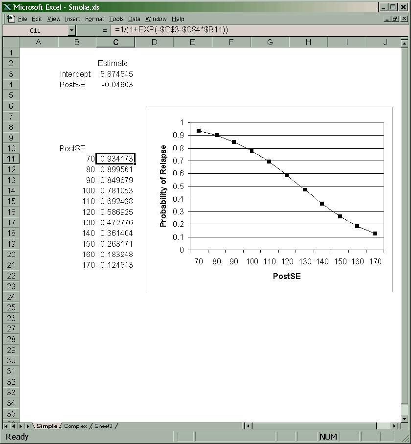
92 - 90 -

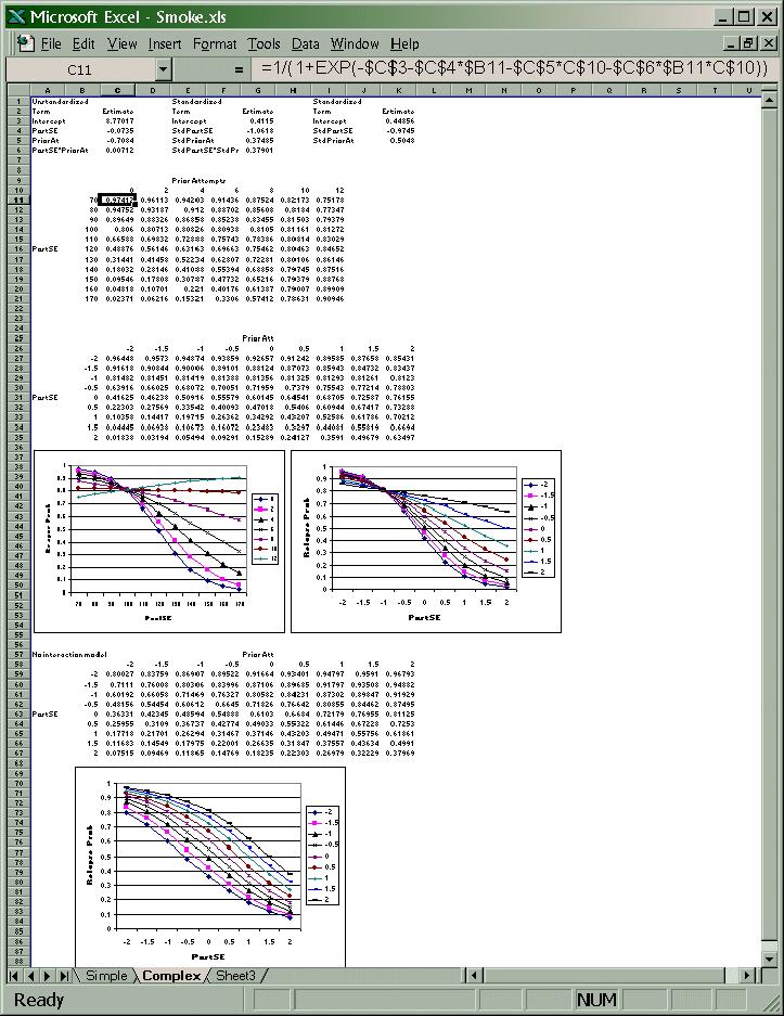
93 - 91 -