NOTES FOR NUMERICAL METHODS MUHAMMAD USMAN HAMID

Transcription

1 NOTES FOR NUMERICAL METHODS MUHAMMAD USMAN HAMID

2 PREFACE In the beginning of university life I used only those books which were recommended by my teachers, soon I realized, that books were not enough to fulfill my requirements then I used every possible way to get any information about my topics. For this purpose one of my best helper was GOOGLE for this I m very thankful to it. I also say thanks to the writers of the books which I used. I also say thank to my parents for their valuable prayers, To my teachers for their guaidance, To my friends for their appreciation, And I dedicated this book to MSc Mathematics Batch the students of INSTITUTES OF LEADERSHIP AND MANAGEMENT SARGODHA. MUHAMMAD USMAN HAMID UNIVERSITY OF SARGODHA PUNJAB, PAKISTAN ( )

3 INTRODUCTION NUMERICAL ANALYSIS Numerical Analysis is the branch of mathematics that provides tools and methods for solving mathematical problems in numerical form. In numerical analysis we are mainly interested in implementation and analysis of numerical algorithms for finding an approximate solution to a mathematical problem. NUMERICAL ALGORITHM A complete set of procedures which gives an approximate solution to a mathematical problem. CRITERIA FOR A GOOD METHOD 1) Number of computations i.e. Addition, Subtraction, Multiplication and Division. 2) Applicable to a class of problems. 3) Speed of convergence. 4) Error management. 5) Stability. STABLE ALGORITHM Algorithm for which the cumulative effect of errors is limited, so that a useful result is generated is called stable algorithm. Otherwise Unstable. NUMERICAL STABILITY Numerical stability is about how a numerical scheme propogate error. NUMERICAL ITERATION METHOD A mathematical procedure that generates a sequence of improving approximate solution for a class of problems i.e. the process of finding successive approximations.

4 ALGORITHM OF ITERATION METHOD A specific way of implementation of an iteration method, including to termination criteria is called algorithm of an iteration method. In the problem of finding the solution of an equation, an iteration method uses as initial guess to generate successive approximation to the solution. CONVERGENCE CRITERIA FOR A NUMERICAL COMPUTATION If the method leads to the value close to the exact solution, then we say that the method is convergent otherwise the method is divergent.i.e. ROUNDING For ; f(x) is an element of F nearest to x and the transformation x f(x) is called Rounding (to nearest). Why we use numerical iterative methods for solving equations? As analytic solutions are often either too tiresome or simply do not exist, we need to find an approximate method of solution. This is where numerical analysis comes into picture. LOCAL CONVERGENCE An iterative method is called locally convergent to a root, if the method converges to root for initial guesses sufficiently close to root. RATE OF CONVERGENCE OF AN ITERATIVE METHOD Suppose that the sequence (x k ) converges to r then the sequence (x k ) is said to converge to r with order of convergence a if there exist a positive constant p such that Thus if, the convergence is linear. If, the convergence is quadratic and so on.where the number a is called convergence factor. REMARK Rate of convergence for fixed point iteration method is linear. Rate of convergence for Newton Raphson method is quadratic. Rate of convergence for Secant method is Super linear.

5 ORDER OF CONVERGENCE OF THE SEQUENCE Let (x 0, x 1,x 2,...)be a sequence that converges to a number a and set Ɛ n =a - x n If there exist a number k and a positive constant c such that Then k is called order of convergence of the sequence and c the asymptotic error constant. CONSISTENT METHOD Let, -, and the function ƒ:*a,b+ R d R + R d may be thought of as the approximate increment per unit step, Or the approximate difference quotient and it defines the method and consider T(x,y:h) is truncation error then the method ƒ is called consistent if T(x,y:h) 0 as h 0 uniformly for (x,y) [a,b] R d PRECISION Precision mean how close are the measurements obtained from successive iterations. ACCURACY Accuracy means how close are our approximations from exact value. DEGREE OF ACCURACY OF A QUADRATURE FORMULA It is the largest positive integer n such that the formula is exact for x k for each (k=0,1,2, n). i.e. Polynomial integrated exactly by method. CONDITION OF A NUMERICAL PROBLEM A problem is well conditioned if small change in the input information causes small change in the output. Otherwise it is ill conditioned. STEP SIZE, STEP COUNT, INTERVAL GAP The common difference between the points i.e. h = = t i+1 - t i is called.

6 ERROR ANALYSIS ERROR Error is a term used to denote the amount by which an approximation fails to equal the exact solution. SOURCE OF ERRORS Numerically computed solutions are subject to certain errors. Mainly there are three types of errors 1. Inherent errors 2. Truncation errors 3. Round Off errors INHERENT (EXPERIMENTAL) ERRORS Errors arise due to assumptions made in the mathematical modeling of problems. Also arise when the data is obtained from certain physical measurements of the parameters of the problem i.e. errors arising from measurements. TRUNCATION ERRORS Errors arise when approximations are used to estimate some quantity. These errors corresponding to the facts that a finite (infinite) sequence of computational steps necessary to produce an exact result is truncated prematurely after a certain number of steps. How Truncation error can be removed? Use exact solution. Error can be reduced by applying the same approximation to a larger number of smaller intervals or by switching to a better approximation. ROUND OFF ERRORS Errors arising from the process of rounding off during computations. These are also called i.e. discarding all decimals from some decimals on.

7 RELATIVE ERRORS If ā is an approximate value of a quantity whose exact value is a then relative error of ā is defined by = EXAMPLE Consider = upto four decimal places then = errors error = = taking as true or exact value. Hence = REMARK I. if is much less than ā II. III. We may also introduce the quantity = a-ā = - and called it the correction ABSOLUTE ERROR If ā is an approximate value of a quantity whose exact value is a then the difference =ā-a is called absolute error of a. ā =a + EXAMPLE If ā = is an approximation to a = 10.5 then the error is = 0.02 ERROR BOUND It is a number β for ā such that ā-a β i.e. β PROBABLE ERROR This is an error estimate such that the actual error will exceed the estimate with probability one half. In other words, the actual error is as likely to be greater than the estimate as less. Since this depends upon the error distribution, it is not an easy target and a rough substitute is often used with the maximum possible error.

8 INPUT ERROR Error arises when the given values (y 0 =f(x 0 ), y 1, y 2,...y n ) are inexact as experimental or computed values usually are. LOCAL ERROR This is the error after first step. i+1 = x(t 0 +h)-x 1 The Local Error is the error introduced during one operation of the iterative process. GLOBAL ERROR This is the error at n-step. n= x(t n ) - x n The Global Error is the accumulation error over many iterations. Note that the Global Error is not simply the sum of the Local Errors due to the non-linear nature of many problems although often it is assumed to be so, because of the difficulties in measuring the global error. LOCAL TRUNCATION ERROR It is the ratio of local error by step size. LTE = REMARK : Floating point numbers are not equally spaced.

9 SOLUTION OF NON-LINEAR EQUATIONS ROOTS (SOLUTION) OF AN EQUATION OR ZEROES OF A FUNCTION Those values of x for which f(x) = 0 is satisfied are called root of an equation. Thus a is root of f(x) = 0 iff f(a) = 0 DEFLATION: It is a technique to compute the other roots of f(x) = 0 ZERO OF MULTIPLICITY A solution p of f(x) = 0 is a zero of multiplicity m of f if for x p we can write f(x) = (x-p) m q(x) where ALGEBRAIC EQUATION The equation f(x) = 0 is called an algebraic equation if it is purely a polynomial in x. e.g. x 3 +5x 2-6x+3 = 0 TRANSCENDENTAL EQUATION The equation f(x) = 0 is called transcendental equation if it contains Trigonometric, Inverse trigonometric, Exponential, Hyperbolic or Logarithmic functions.e.g. i. M = e-esinx ii. ax 2 + log(x-3) +exsinx = 0 PROPERTIES OF ALGEBRAIC EQUATIONS 1. Every algebraic equation of degree n has n and only n roots.e.g. x 2-1=0 has distinct roots i.e. 1, -1 x 2 +2x+1 = 0 has repeated roots i.e. -1, -1 x 2 +1 = 0 has complex roots i.e. +і, -і 2. Complex roots occur in pair. i.e. (a+bі) and (a-bі) are roots of f(x)=0 3. If x = a is a root f(x)=0, a polynomial of degree n then (x-a) is factor of f(x)=0 on dividing f(x) by (x-a) we obtain polynomial of degree (n-1).

10 DISCARTS RULES OF SIGNS The number of positive roots of an algebraic equation f(x)=0 with the real coefficient cannot exceed the number of changes in sign of the coefficient in f(x)=0. e.g. x 3-3x 2 +4x-5=0 changes its sign 3-time, so it has 3 roots. Similarly, the number of negative roots of f(x)=0 cannot exceed the number of changes in sign of the coefficient of f(-x) =0 e.g. -x 3-3x 2-4x-5=0 does not changes its sign, so it has no negative roots. REMARK There are two types of methods to find the roots of Algebraic and Transcendental equations. (i) DIRECT METHODS (ii) INDIRECT (ITERATIVE) METHODS DIRECT METHODS 1. Direct methods give the exact value of the roots in a finite number of steps. 2. These methods determine all the roots at the same time assuming no round off errors. 3. In the category of direct methods; Elimination Methods are advantageous because they can be applied when the system is large. INDIRECT (ITERATIVE) METHODS 1. These are based on the concept of successive approximations. The general procedure is to start with one or more approximation to the root and obtain a sequence of iterates x which in the limit converges to the actual or true solution to the root. 2. Indirect Methods determine one or two roots at a time. 3. Rounding error have less effect 4. These are self-correcting methods. 5. Easier to program and can be implemented on the computer. REMEMBER: Indirect Methods are further divided into two categories I. BRACKETING METHODS II. OPEN METHODS

11 BRACKETING METHODS These methods require the limits between which the root lies. e.g. Bisection method, False position method. OPEN METHODS These methods require the initial estimation of the solution. e.g. Newton Raphson method. ADVANTAGES AND DISADVANTAGES OF BRACKETING METHODS Bracket methods always converge. The main disadvantage is, if it is not possible to bracket the root, the method cannot applicable. GEOMETRICAL ILLUSTRATION OF BRACKET FUNCTIONS In these methods we choose two points x n and x n-1 such that f(x n ) and f(x n-1 ) are of opposite signs. Intermediate value property suggests that the graph of y=f(x) crosses the x-axis between these two points, therefore a root (say) x=x r lies between these two points. REMARK Always set your calculator at radian mod while solving Transcendental or Trigonometric equations. How to get first approximation? We can find the approximate value of the root of f(x)=0 by Graphical method or by Analytical method. INTERMEDIATE VALUE THEOREM Suppose f is continuous on [a, b+ and f(a) f(b) then given a number ƛ that lies between f(a) and f(b) then there exist a point c such that a<c<b with

12 BISECTION METHOD Bisection method is one of the bracketing methods. It is based on the Intermediate value theorem The idea behind the method is that if f(x) c (a,b) such that f(c)=0 C [a, b] and f(a).f(b)<0 then there exist a root This method also known as BOLZANO METHOD (or) BINARY SECTON METHOD. ALGORITHM For a given continuous function f(x) 1. Find a,b such that f(a).f(b)<0 (this means there is a root r (a,b) such that f(r)=0 2. Let c = (mid-point) 3. If f(c)=0; done (lucky!) 4. Else; check if or 5. Pick that interval [a, c] or [c, b] and repeat the procedure until stop criteria satisfied. STOP CRITERIA 1. Interval small enough. 2. f(c n ) almost zero 3. Maximum number of iteration reached 4. Any combination of previous ones

13 CONVERGENCE CRITERIA No. of iterations needed in the bisection method to achieve certain accuracy Consider the interval [a 0,b 0 ],, c 0 = and let r (a 0,b 0 ) be a root then the error is 0 = r-c 0 Denote the further intervals as [a n,b n ] for iteration number n then n= r-c n = If the error tolerance is we require n then After taking logarithm log (b 0 -a 0 ) nlog2 log (2 ) n n (which is required) MERITS OF BISECTION METHOD 1. The iteration using bisection method always produces a root, since the method brackets the root between two values. 2. As iterations are conducted, the length of the interval gets halved. So one can guarantee the convergence in case of the solution of the equation. 3. Bisection method is simple to program in a computer. DEMERITS OF BISECTION METHOD 1. The convergence of bisection method is slow as it is simply based on halving the interval. 2. Cannot be applied over an interval where there is discontinuity. 3. Cannot be applied over an interval where the function takes always value of the same sign. 4. Method fails to determine complex roots (give only real roots) 5. If one of the initial guesses a 0 or b 0 is closer to the exact solution, it will take larger number of iterations to reach the root.

14 EXAMPLE Solve x 3-9x+1 for roots between x=2 and x=4 SOLUTION X 2 4 f(x) Since f (2). f (4) <0 therefore root lies between 2 and 4 (1) x r = = 3 so f(3) = 1 (+ve) (2) For interval [2,3] ; x r = = 2.5 f (2.5) = (-ve) (3) For interval [2.5,3]; x r = (2.5+3)/2 = 2.75 f (2.75) = (-ve) (4) For interval [2.75,3]; x r = (2.75+3)/2 = f (2.875) = (-ve) (5) For interval [2.875,3]; x r = ( )/2 = f (2.9375) = (-ve) (6) For interval [2.9375,3]; x r = ( )/2 = f (2.9688) = (+ve) (7) For interval [2.9375,2.9688]; x r = ( )/2 = f (2.9532) = (+ve) (8) For interval [2.9375,2.9532]; x r = ( )/2 = f (2.9453) = Hence root is because roots are repeated.

15 EXAMPLE Use bisection method to find out the roots of the function describing to drag coefficient of parachutist given by f(c) = [1-exp( c)]-40 Where c=12 to c=16 perform at least two iterations. SOLUTION Given that f(c) = [1-exp( c)]-40 X f(x) Since f (14). f (15) <0 therefore root lie between 14 and 15 X r = = 14.5 So f(14.5) = Again f (14.5). f (15) <0 therefore root lie between 14.5 and 15 x r = = So f(14.75) = These are the required iterations EXAMPLE Explain why the equation e x = x has a solution on the interval [0,1]. Use bisection to find the root to 4 decimal places. Can you prove that there are no other roots? SOLUTION If f(x) = e x x, then f(0) = 1, f(1) = 1/e 1 < 0, and hence a root is guaranteed by the Intermediate Value Theorem. Using Bisection, the value of the root is x? = Since f 0 (x) = e x 1 < 0 for all x, the function is strictly decreasing, and so its graph can only cross the x axis at a single point, which is the root.

16 FALSE POSITION METHOD This method also known as REGULA FALSI METHOD,, CHORD METHOD,, LINEAR INTERPOLATION and method is one of the bracketing methods and based on intermediate value theorem. This method is different from bisection method. Like the bisection method we are not taking the mid-point of the given interval to determine the next interval and converge faster than bisection method. ALGORITHM Given a function f(x) continuous on an interval [a 0,b 0 ] and satisfying f(a 0 ).f(b 0 )<0 for all n = 0,1,2,3.. then Use following formula to next root = f(x f) We can also use x r = x n+1,,, x f = x n,,, x i = x n-1 STOPING CRITERIA 1. Interval small enough. 2. f(c n ) almost zero 3. Maximum number of iteration reached 4. Same answer. 5. Any combination of previous ones

17 EXAMPLE Using Regula Falsi method Solve x 3-9x+1 for roots between x=2 and x=4 SOLUTION X 2 4 f(x) Since f(2).f(4)<0 therefore root lies between 2 and 4 Using formula = x f - f(x f ) For interval [2,4] we have x r 29 Which implies (-ve) Similarly, other terms are given below Interval x r F(x r ) [2.4737,4] [2.7399,4] [2.8613,4] [2.9111,4] [2.9306,4] [2.9382,4] [2.9412,4] [2.9422,4] [2.9426,4] [2.9426,2.9439] [2.9426,2.9439]

18 EXAMPLE Using Regula Falsi method to find root of equation places, after 3 successive approximations. upto four decimal SOLUTION X F(X) Since f(1).f(2)<0 therefore root lies between 1 and 2 Using formula Xr= x f - f(x f ) For interval [1,2] we have x r =2- Which implies f(2.4737)=0.0424(+ve) = Similarly, other terms are given below Interval x r F(x r ) [1,1.3275] [1,1.3037] Hence the root is KEEP IN MIND Calculate this equation in Radian mod If you have log then use natural log. If you have then use simple log.

19 GENERAL FORMULA FOR REGULA FALSI USING LINE EQUATION Equation of line is Put (x,0) i.e. y=0 Hence first approximation to the root of f(x) =0 is given by We observe that f(x n-1 ), f(x n+1 ) are of opposite sign so, we can apply the above procedure to successive approximations.

20 SECANT METHOD The secant method is a simple variant of the method of false position which it is no longer required that the function f has opposite signs at the end points of each interval generated, not even the initial interval. In other words, one starts with two arbitrary initial approximations with and continues ; n=1,2,3,4. This method also known as QUASI NEWTON S METHOD. ADVANTAGES 1. No computations of derivatives 2. One f(x) computation each step 3. Also rapid convergence than Falsi method Example 1 Use Secant method to find the root of the function f(x) = cosx + 2sinx + x 2 to 5 decimal places. Don t forget to adjust your calculator for radians. Solution: A closed form solution for x does not exist so we must use a numerical technique. The Secant method is given using the iterative equation:, (1) We will use x 0 = 0 and x 1 = 0.1 as our initial approximations and substituting in (1), we have The continued iterations can be computed as shown in Table 1 which shows a stop at iteration no. 5 since the error is x 5 x 4 < 10 5 resulting in a root of x = Table 1: Iterations for Example-1 Iteration no. x n 1 x n x n+1 using (1) f(x n+1) x n+1 x n 1 x 0 = 0 x 1 =

21 Example-2: Use Secant method to find the root of the function f(x) = x 3 4 to 5 decimal places. Solution Since the Secant method is given using the iterative equation in (1). Starting with an initial value x 0 = 1 and x 1 = 1.5, using (1) we can compute The continued iterations can be computed as shown in Table 2 which shows a stop at iteration no. 5 since the error is x 5 x 4 < 10 5 resulting in a root of x = , Table 2: Iterations for Example-2 Iteration no. x n 1 x n x n+1 using (1) f(x n+1) x n+1 x n 1 x 0 = 1 x 1 = < 10 5 Example-3: Use Secant method to find the root of the function f(x) = 3x + Sinx e x to 5 decimal places. Use x0 = 0 and x1 = 1. Solution Using (1) we can compute The continued iterations can be computed as shown in Table 3 which shows a stop at iteration no. 6 since the error is x6 x5 < 10 5 resulting in a root of x = Table 3: Iterations for Example-3 Iteration xn 1 xn xn+1 using (1) f(xn+1) xn+1 xn no. 1 x0 = 0 x1 = < 10 5

22 Example-4: Solve the equation exp( x) = 3log(x) to 5 decimal places using secant method, assuming initial guess x0 = 1 and x1 = 2. Solution Let f(x) = exp( x) 3log(x), to solve the given, it is now equivalent to find the root of f(x). Using (1) we can compute x2 = The continued iterations can be computed as shown in Table 4 which shows a stop at iteration no. 5 since the error is x5 x4 < 10 5 resulting in a root of x = , Table 4: Iterations for Example-4 Iteration xn 1 xn xn+1 using (1) f(xn+1) xn+1 xn no. 1 x0 = 1 x1 = < 10 5 FIXED POINT The real number x is a fixed point of the function f if f(x) =x The number x= is an approximate fixed point of f(x) = cosx REMARK Fixed point are roughly divided into three classes ASYMPTOTICALLY STABLE: with the property that all nearby solutions converge to it. STABLE: All nearby solutions stay nearby. UNSTABLE: Almost all of whose nearby solutions diverge away from the fixed point

23 FIXED POINT ITERATION METHOD ALGORITHM 1. Consider f(x) =0 and transform it to the form x= (x) 2. Choose an arbitrary x 0 3. Do the iterations x k+1 = ; k=0,1,2,3. STOPING CRITERIA Let be the tolerance value Maximum number of iterations reached. 4. Any combination of above. CONVERGENCE CRITERIA Let x be exact root such that r=f(x) out iteration is x n+1 = f(x n ) Define the error n = x n -r Then (Where ; since f is continuous) OBSERVATIONS If < 1, error decreases, the iteration converges (linear convergence) If 1, error increases, the iteration diverges. REMEMBER: If < 1 in questions then take that point as initial guess.

24 EXAMPLE Find the root of equation iteration method. correct to three decimal points using fixed point SOLUTION Given that X F(X) Root lies between 1 and 2 Now (-sinx) (-sinx) Now Here we will take x 0 as mid-point. So If by putting 1 we get φ (x) < 1 then take it as x 0 if not then check for 2 rather take their midpoint X 0 = X 1 = F(x 1 ) = X 2 = = F(x 2 ) = X 3 = F(x 3 ) = x 4 = F(x 4 ) = X 5 = F(x 5 ) = X 6 = F(x 6 ) = X 7 = F(x 7 ) = X 8 = F(x 8 ) = X 9 = F(x 9 ) = Hence the real root is

25 EXAMPLE Find the root of equation iteration method. correct to four decimal points using fixed point SOLUTION Given that X 0 1 F(X) Root lies between 0 and 1 Now Now since is less than 1 therefore x 0 = 0 Now X 1 = F(x 1 ) = X 2 = F(x 2 ) = X 3 = F(x 3 ) = x 4 = F(x 4 ) = Hence the real root is

26 NEWTON RAPHSON METHOD The Newton Raphson method is a powerful technique for solving equations numerically. It is based on the idea of linear approximation. Usually converges much faster than the linearly convergent methods. ALGORITHM The steps of Newton Raphson method to find the root of an equation f(x) =0 are Evaluate Use an initial guess (value on which f(x) and estimate the new value of the root x n+1 as becomes (+ve) of the roots x n to STOPING CRITERIA 1. Find the absolute relative approximate error as 2. Compare the absolute error with the pre-specified relative error tolerance s. 3. If a > s then go to next approximation. Else stop the algorithm. 4. Maximum number of iterations reached. 5. Repeated answer. CONVERGENCE CRITERIA Newton method will generate a sequence of numbers (x n ) ; n x * of f if 0, that converges to the zero f is continuous. x * is a simple zero of f. x 0 is close enough to x *

27 When the Generalized Newton Raphson method for solving equations is helpful? To find the root of f(x)=0 with multiplicity p the Generalized Newton formula is required. What is the importance of Secant method over Newton Raphson method? Newton Raphson method requires the evaluation of derivatives of the function and this is not always possible, particularly in the case of functions arising in practical problems. In such situations Secant method helps to solve the equation with an approximation to the derivatives. Why Newton Raphson method is called Method of Tangent? In this method we draw tangent line to the point P 0 (x 0,f(x 0 )). The (x,0) where this tangent line meets x-axis is 1 st approximation to the root. Similarly, we obtained other approximations by tangent line. So, method also called Tangent method. Difference between Newton Raphson method and Secant method. Secant method needs two approximations x 0,x 1 to start, whereas Newton Raphson method just needs one approximation i.e. x 0 Newton Raphson method converges faster than Secant method. Newton Raphson method is an Open method, how? Newton Raphson method is an open method because initial guess of the root that is needed to get the iterative method started is a single point. While other open methods use two initial guesses of the root but they do not have to bracket the root.

28 INFLECTION POINT For a function f(x) the point where the concavity changes from up-to-down or down-to-up is called its Inflection point. e.g. f(x) = (x-1) 3 changes concavity at x=1,, Hence (1,0) is an Inflection point. DRAWBACKS OF NEWTON S RAPHSON METHOD Method diverges at inflection point. For f(x)=0 Newton Raphson method reduce. So one must be avoid division by zero. Rather method not converges. Root jumping is another drawback. Results obtained from Newton Raphson method may oscillate about the Local Maximum or Minimum without converging on a root but converging on the Local Maximum or minimum. Eventually, it may lead to division by a number close to zero and may diverge. The requirement of finding the value of the derivatives of f(x) at each approximation is either extremely difficult (if not possible) or time consuming.

29 FORMULA DARIVATION FOR NR-METHOD Given an equation f(x) = 0 suppose x 0 is an approximate root of f(x) = 0 Let Where h is the small; exact root of f(x)=0 Then By Taylor theorem Since h is small therefore neglecting higher terms we get Similarly This is required Newton s Raphson Formula.

30 EXAMPLE Apply Newton s Raphson method for correct to three decimal places. SOLUTION Using formula at Similarly n Hence root is REMARK 1. If two are more roots are nearly equal, then method is not fastly convergent. 2. If root is very near to maximum or minimum value of the function at the point, NRmethod fails.

31 EXAMPLE Apply Newton s Raphson method for correct to two decimal places. SOLUTION For interval X f(x) Root lies between 6 and 7 and let x 0 =7 Using formula Thus Similarly n Hence root is 6.08

32 GEOMETRICAL INTERPRETATION (GRAPHICS) OF NEWTON RAPHSON FORMULA Suppose the graph of function y=f(x) crosses x-axis at then is the root of equation. CONDITION Choose x 0 such that and have same sign. If ( ) is a point then slope of tangent at Now equation of tangent is. (i) Since ( ) as we take x 1 as exact root (i) Which is first approximation to the root. If P 1 is a point on the curve corresponding to x 1 then tangent at P 1 cuts x-axis at P 1 (x 2, 0) which is still closer to than x 1. Therefore x 2 is a 2 nd approximation to the root. Continuing this process, we arrive at the root.

33 CONDITION FOR CONVERGENCE OF NR-METHOD Since by Newton Raphson method And by General Iterative formula Comparing (1) and (2) Since by iterative method condition for convergence is So, ( ) - ( ) ( ) Using in (3) we get ( ) ( ) Which is required condition for convergence of Newton Raphson method, provided that initial approximation x 0 is choose sufficiently close to the root and are continuous and bounded in any small interval containing the root.

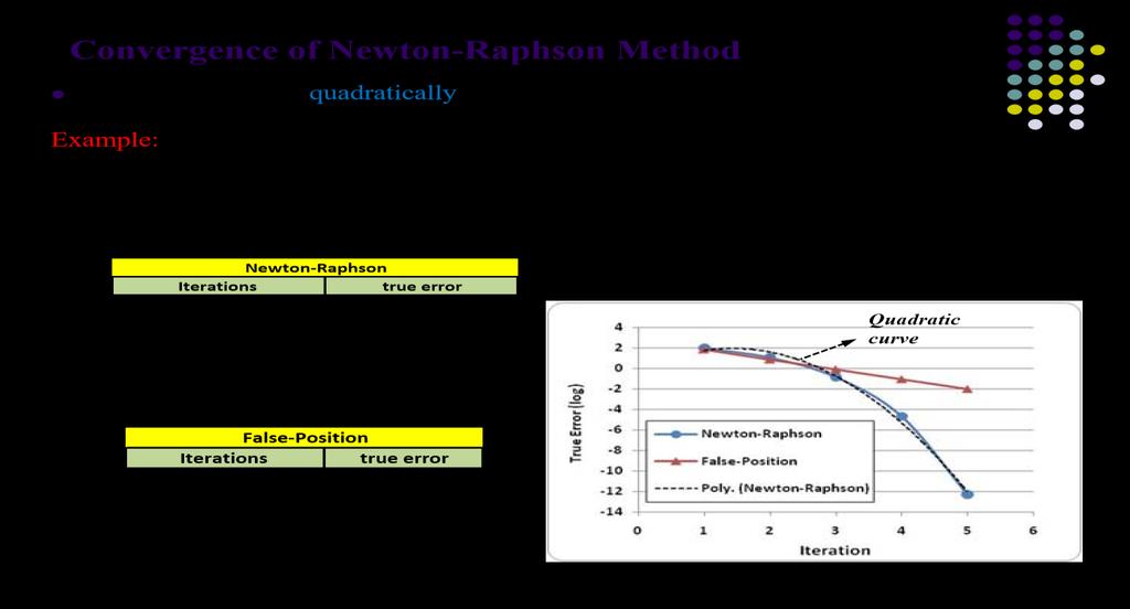
34 NEWTON RAPHSON METHOD IS QUADRATICALLY CONVERGENT (OR) NEWTON RAPHSON METHOD HAS SECOND ORDER CONVERGENCE (OR) ERROR FOR NEWTON RAPHSON METHOD Let be the root of f(x) =0 and ( * If we can prove that where k is constant then p is called order of convergence of iterative method then we are done. Since by Newton Raphson formula we have Then using (1) in it Since by Taylor expansion we have Since is root of f(x) therefore

35 , - After neglecting higher terms,, - -, It shows that Newton Raphson method has second order convergence Or Converges quadratically.

36

37 NEWTON RAPHSON EXTENDED FORMULA (CHEBYSHEVES FORMULA OF 3 RD ORDER) Consider f(x) =0. Expand f(x) by Taylor series in the neighborhood of x 0. We obtain after retaining the first term only. This the first approximation to the root therefore Again expanding f(x) by Taylor Series and retaining the second order term only Using eq. (1) in (2) we get, - 6 7, -, -, - This is Newton Raphson Extended formula. Also known as Chebysheves formula of third order

38 NEWTON SCHEME OF ITERATION FOR FINDING THE SQUARE ROOT OF POSITION NUMBER The square root of N can be carried out as a root of the equation Here Using Newton Raphson formula, - This is required formula. QUESTION Evaluate by Newton Raphson formula. SOLUTION Let Here X F(x) Root lies between 3 and 4 and x 0 =4 Now using formula For n= =3.5 For n= Similarly Hence

39 NEWTON SCHEME OF ITERATION FOR FINDING THE pth ROOT OF POSITION NUMBER N Consider Here Since by Newton Raphson formula. / [ ] [ ], - Required formula for pth root. QUESTION Obtain the cube root of 12 using Newton Raphson iteration. SOLUTION Consider Here and For interval X F(x) Root lies between 2 and 3 and x 0 =3 Since by Newton Raphson formula for pth root., - 0 1, - Put n=0 [ ] 0 1 Similarly Hence

40 DARIVATION OF NEWTON RAPHSON METHOD FROM TAYLOR SERIES Newton Raphson method can also be derived from Taylor series. For the general function f(x) Taylor series is As an approximation, taking only the first two terms of the R.H.S. And we are seeking a point where f(x) =0 That is If we assume f (x n+1 ) =0 This gives This is the formula for Newton Raphson Method.

41 THE SOLUTION OF LINEAR SYSTEM OF EQUATIONS A system of m linear equations in n unknowns equations of the form is a set of the.. Where the coefficients and are given numbers. The system is said to be homogeneous if all the are zero. Otherwise it is said to be non-homogeneous. SOLUTION OF LINEAR SYSTEM EQUATIONS A solution of system is a set of numbers equations. which satisfy all the m PIVOTING: Changing the order of equations is called pivoting. We are interested in following types of Pivoting 1. PARTIAL PIVOTING 2. TOTAL PIVOTING PARTIAL PIVOTING In partial pivoting we interchange rows where pivotal element is zero. In Partial Pivoting if the pivotal coefficient happens to be zero or near to zero, the i th column elements are searched for the numerically largest element. Let the j th row (j>i) contains this element, then we interchange the i th equation with the j th equation and proceed for elimination. This process is continued whenever pivotal coefficients become zero during elimination.

42 TOTAL PIVOTING In Full (complete, total) pivoting we interchange rows as well as column. In Total Pivoting we look for an absolutely largest coefficient in the entire system and start the elimination with the corresponding variable, using this coefficient as the pivotal coefficient (may change row and column). Similarly, in the further steps. It is more complicated than Partial Pivoting. Partial Pivoting is preferred for hand calculation. Why is Pivoting important? Because Pivoting made the difference between non-sense and a perfect result. PIVOTAL COEFFICIENT For elimination methods (Guass s Elimination, Guass s Jordan) the coefficient of the first unknown in the first equation is called Pivotal Coefficient. BACK SUBSTITUTION The analogous algorithm for upper triangular system Ax=b of the form (, (, (, Is called Back Substitution. The solution x i is computed by FORWARD SUBSTITUTION The analogous algorithm for lower triangular system Lx=b of the form (, (, (, Is called Forward Substitution. The solution x i is computed by

43 THINGS TO REMEMBER Let the system is given If then system is called non homogenous system of linear equation. If then then system is called homogenous system of linear equation. If the system has solution then this system is called consistent. If the system has no solution then this system is called inconsistent. RANK OF A MATRIX The rank of a matrix A is equal to the number of non zero rows in its echelon form or the order of in the conical form of A. KEEP IN MIND TYPE I: when number of equations is equal to the number of variables and the system is non homogeneous then unique solution of the system exists if matrix A is non- singular after applying row operation. TYPE II: when number of equations is not equal (may be equal) to the number of variables and the system is non homogeneous then system has a solution if TYPE III: a system of m homogeneous linear equations in n unknown has a non- trivial solution if where n is number of columns of A. TYPE IV: if then infinite solution exists TYPE V: if then no solution exists

44 GUASS ELIMINATION METHOD ALGORITHM In the first stage, the given system of equations is reduced to an equivalent upper triangular form using elementary transformation. In the second stage, the upper triangular system is solved using back substitution procedure by which we obtain the solution in the order REMARK Guass s Elimination method fails if any one of the Pivotal coefficient become zero. In such a situation, we rewrite the equation in a different order to avoid zero Pivotal coefficients. QUESTION Solve the following system of equations using Elimination Method. SOLUTION We can solve it by elimination of variables by making coefficients same. Multiply (i) by 2 and subtracted by (ii) Adding (i) and (iii) Now eliminating y Multiply (iv) by 3 then subtract from (v) Using z in (iv) we get and Using y, z in (i) we get Hence solution is

45 QUESTION Solve the following system of equations by Guass s Elimination method with partial pivoting. SOLUTION [ ] 6 7 [ ] [ ] 6 7 [ ] * [ ] [ ] 6 7 [ ] 6 7 [ ] [ ] 2 nd row cannot be used as pivot row as a 22 =0, So interchanging the 2 nd and 3 rd row we get 6 7 [ ] [ ] Using back substitution

46 QUESTION Solve the following system of equations using Guass s Elimination Method with partial pivoting. SOLUTION [ ] [ ] [ ] [ ] [ ] [ ] [ ] [ ] [ ] [ ] [ ] [ ] [ ] [ ] [ ] and [ ] [ ] [ ]

47 [ ] [ ] [ ] [ ] [ ] [ ] Hence required solutions are,

48 GUASS JORDAN ELIMINATION METHOD The method is based on the idea of reducing the given system of equations to a diagonal system of equations where is the identity matrix, using row operation. It is the verification of Gauss s Elimination Method. ALGORITHM 1) Make the elements below the first pivot in the augmented matrix as zeros, using the elementary row transformation. 2) Secondly make the elements below and above the pivot as zeros using elementary row transformation. 3) Lastly divide each row by its pivot so that the final matrix is of the form [ ] Then it is easy to get the solution of the system as Partial Pivoting can also be used in the solution. We may also make the pivot as 1 before performing the elimination. ADVANTAGE/DISADVANTAGE The Guass s Jordan method looks very elegant as the solution is obtained directly. However, it is computationally more expensive than Guass s Elimination. Hence we do not normally use this method for the solution of the system of equations. The most important application of this method is to find inverse of a non-singular matrix. What is Gauss Jordan variation? In this method Zeroes are generated both below and above each pivot, by further subtractions. The final matrix is thus diagonal rather than triangular and back substitution is eliminated. The idea is attractive but it involves more computing than the original algorithm, so it is little used.

49 QUESTION Solve the system of equations using Elimination method ANSWER [ ] [ ] [ ] [ ] [ ] [ ] [ ] Hence solutions are

50 MATRIX INVERTION A matrix is said to be non-singular (or Invertible) if a matrix exists with - then matrix is called the inverse of. A matrix without an inverse is called Singular (or Non-invertible) MATRIX INVERSION THROUGH GUASS ELIMINATION 1. Place an identity matrix, whose order is same as given matrix. 2. Convert matrix in upper triangular form. 3. Take largest value as Pivot. 4. Using back substitution get the result. NOTE: In order to increase the accuracy of the result, it is essential to employ Partial Pivoting. In the first column use absolutely largest coefficient as the pivotal coefficient (for this we have to interchange rows if necessary). Similarly, for the second column and vice versa. MATRIX INVERSION THROUGH GUASS JORDAN ELIMINATION 1. Place an identity matrix, whose order is same as given matrix. 2. Convert matrix in upper triangular form. 3. No need to take largest value as Pivot. 4. Using back substitution get the result. QUESTION : Find inverse using Guass Elimination Method [ ] ANSWER [ ] [ ] * +

51 [ ] [ ] [ ] [ ] [ ] [ ] [ ] Hence [ ] [ ]

52 QUESTION Find inverse using Guass s Jordan Elimination Method [ ] ANSWER [ ] [ ] [ ] [ ] * + [ ] Hence [ ] [ ]

53 QUESTION: Find if [ ] SOLUTION: we first find the co-factor of the elements of A a 11 = = 3 a 12 = = 1 a 13 = -2 a 21 = = -2 a 22 = = -1 a 23 = a 31 = a 32 = a 33 = Thus [ ] [ ] [ ] [ ] [ ] So [ ] after putting the values.

54 HESSENBERG MATRIX: Matrix in which either the upper or lower triangle is zero except for the elements adjacent to the main diagonal. If the upper triangle has the zeroes, the matrix is the Lower Heisenberg and vice versa. SPARSE: known to be zero. A coefficient matrix is said to be sparse if many of the matrix entries are ORTHOGONAL MATRIX: A matrix M is called orthogonal if PERMUTATION MATRIX A matrix [ ] is a permutation matrix obtained by rearranging the rows of the identity matrix. This gives a matrix with precisely one non-zero entry in each row and in each column and each non-zero entry is 1 For example [ ] CONVERGENT MATRIX We call a matrix M convergent if for each i, j=0, 1, 2 n Consider * + * + Then and is convergent. LOWER TRIANGULATION MATRIX A matrix having only zeros above the diagonal is called Lower Triangular matrix. (OR) A matrix L is lower triangular if its entries satisfy i.e. [ ]

55 UPPER TRIANGULATION MATRIX A matrix having only zeros below the diagonal is called Upper Triangular matrix. (OR) A matrix U is upper triangular if its entries satisfy i.e. [ ] CROUTS REDUCTION METHOD In linear Algebra this method factorizes a matrix as the product of a Lower Triangular matrix and an Upper Triangular matrix. Method also named as Cholesky s reduction method, triangulation method, or LU-decomposition (Factorization) ALGORITHM For a given system of equations 1. Construct the matrix A 2. Use A=LU (without pivoting) and PA=LU (with pivoting) where P is the pivoting matrix and find 3. Use formula AX=B where X is the matrix of variables and B is the matrix of solution of equations. 4. Replace AX=B by LUX=B and then put UX=Z i.e. LZ=B 5. Find the values of then use Z=UX find ; i=1, 2, 3,.n ADVANTAGE/LIMITATION (FAILURE) 1. Cholesky s method widely used in Numerical Solution of Partial Differential Equation. 2. Popular for Computer Programming. 3. This method fails if in that case the system is Singular.

56 QUESTION Solve the following system of equations using Crout s Reduction Method ANSWER Let [ ] Step I. One of the diagonals of L or U must be 1, -, -, - [ ] [ ] [ ] After multiplication on R.H.S [ ] [ ] ( * ( *

57 . /. /. / Step II. Put, -, -, -, -, -, -, - Put [U] [X] = [Z], -, -, - [ ] [ ] [ ] [ ] [ ] [ ]. / ( * Step III. Since [U][X] = [Z] [ ] [ ] [ ] [ ] [ ] [ ] ( *. /. /. / Hence required solutions are,

58 DIAGONALLY DOMINANT SYSTEM Consider a square matrix * + then system is said to be Diagonally Dominant if If we remove equality sign, then A is called strictly diagonally dominant and A has the following properties A is regular, invertible, its inverse exist and Ax = b has a unique solution. Ax = b can be solved by Gaussian Elimination without Pivoting. For example [ ] [ ] Then non- symmetric matrix A is strictly diagonally dominant because But B and are not strictly diagonally dominant (Check!) NORM: A norm measures the size of a matrix. Let Iff x =0 then Where a is constant. i.e. Triangular inequality INFINITY NORM The infinity (maximum) norm of a matrix X is Consider [ ] [ ]

59 EUCLIDEAN NORM The Euclidean norm for the matrix X is [ ] We name it Euclidean norm because it represents the usual notation of distance from the origin in case x is in Consider [ ] Take square of each element, add &then square root USEFUL DEFINATIONS Let be an approximate solution of the linear system Ax =b then The residual is the vector The backward error is the norm of residual The forward error is The relative backward error is The relative forward error is And error magnification factor is equals to CONDITION NUMBER For a square matrix A condition number is the maximum possible error magnification factor for solving Ax=b Or The condition number of the matrix is defined as Remember: Identity matrix has the lowest condition number.

60 ILL CONDITION LINEAR SYSTEM In practical application small change in the coefficient of the system of equations sometime gives the large change in the solutions of system. This type of system is called ill-condition linear system otherwise it is well-condition. PROCEDURE (TEST, MEASURE OF CONDITION NUMBER) Find determinant. If system is ill condition, then determinant will be very small. Find condition number. If condition number is very large then system of condition is ill-condition rather it is well-condition. Also determinant will be small. EXAMPLE: Consider ( ) Now condition number = = (very large) Since condition Number is very large therefore system will be ill-condition. Ill Conditioning Example Here is a simple example of ill conditioning. Suppose that Ax = b is supposed to be 2x+6y= 8 and 2x y= The actual solution is x = 1, y = 1. Suppose further that due to representation error, the system on the machine is changed slightly to 2x+6y= 8 and 2x y= The solution to this system is x = 10, y = 2, so you think the answer is (10, 2). When you check the answer by plugging these values into the actual system, you get 2(10) + 6( 2)=8 and 2(10) ( 2)= This seems to be acceptable, but of course (10, 2) is very far from the actual solution (1,1). This indicates that the system is badly ill conditioned. Here are some things to consider if you have an ill conditioned system:

61 To identify if the matrix is ill conditioned, you can try 2 things. First, compute cond(a). This is relatively expensive and sometimes hard to interpret because the value may be in an intermediate range. Second, you can introduce deliberate representation errors by slightly perturbing one or more elements in A. Call the new matrix A 0, and solve A 0 x 0 = b. If x x 0, then there is probably no ill conditioning. The danger here is that you might be unlucky, and chose the wrong element to perturb. But if you try this several times with different elements and all the solutions are about the same, then you have confidence that the matrix is well conditioned. EXAMPLE If the system really is ill conditioned, there is no simple fix. Consider using Singular Value Decomposition (SVD Ill-Conditioned Matrices Consider systems x + y = 2 THEN x y = 2 x y = The system on the left has solution x = 2, y = 0 while the one on the right has solution x = 1, y = 1. The coefficient matrix is called ill-conditioned because a small change in the constant coefficients results in a large change in the solution. A condition number, defined in more advanced courses, is used to measure the degree of ill-conditioning of a matrix ( 4004 for the above). In the presence of rounding errors, ill-conditioned systems are inherently difficult to handle. When solving systems where round-off errors occur, one must avoid ill-conditioned systems whenever possible; this means that the usual row reduction algorithm must be modified. Consider the system:.001x + y = 1 AND x + y = 2 We see that the solution is x = 1000/999 1, y = 998/999 1 which does not change much if the coefficients are altered slightly (condition number 4). The usual row reduction algorithm, however, gives an ill-conditioned system. Adding a multiple of the first to the second row gives the system on the left below, then dividing by 999 and rounding to 3 places on 998/999 = gives the system on the right:.001x + y = 1.001x + y = 1 999y = 998 y = 1.00 The solution for the last system is x = 0,y = 1 which is wildly inaccurate (and the condition number is 2002). This problem can be avoided using partial pivoting. Instead of pivoting on the first non-zero element, pivot on the largest pivot (in absolute value) among those available in the column. In the example above, pivot on the x, which will require a permute first: x + y = 2 x + y = 2 x + y = 2.001x + y = 1.999y =.998 y = 1.00 where the third system is the one obtained after rounding. The solution is a fairly accurate x = 1.00,y = 1.00 (and the condition number is 4).

62 JACOBI S METHOD Method also known as iterative method, simultaneous displacement method. We want to solve Ax = b where and n is very large, A is Sparse (with a large percent of zero entries) as well as A is structured (i.e. the product Ax can be computed efficiently). For this purpose, we can easily use Jacoby s. ALGORITHM We want to solve Ax=b writes it out { Rewrite it in another way { ( ) Or in compact form ( ) This gives the Jacoby s iteration. Choose a start point (initial guess) i.e. Apply where and B can be defined as 8 STOP CRITERIA close enough to for example for certain vector norms. Residual is small for example

63 CONVERGENC CRITERIA Sufficient condition for the convergence of Jacobi s is Jacobi method also called method of simultaneous displacement why? Because no element of is in this iteration until every element is computed. KEEP IN MIND Jacobi method is valid only when all a i s are non-zeroes. (OR) the elements can rearrange for measuring the system according to condition. It is only possible if [A] is invertible i.e. inverse of A exist. For fast convergence system should be diagonally dominant. Must make two vectors for the computation and System (method) is important for parallel computing. QUESTION: Find the solution of the system of equation using Jacobi iterative method for the first five iterations. ANSWER

64 Taking initial guess as (0, 0, 0) and using formula Put k = 0 for first iteration Put k = 1 for second iteration ( ) Put k = 2 for third iteration ( ) Put k = 3 for fourth iteration ( )

65 Put k = 4 for fifth iteration ( ) ( ) GUASS SEIDEL ITERATION METHOD Guass s Seidel method is an improvement of Jacobi s method. This is also known as method of successive displacement. ALGORITHM In this method we can get the value of from first equation and we get the value of by using in second equation and we get by using and in third equation and so on. ABOUT THE ALGORITHM Need only one vector for both and save memory space. Not good for parallel computing. Converge a bit faster than Jacobi s.

66 How Jacobi method is accelerated to get Guass Seidel method for solving system of Linear Equations. In Jacobi method the (r+1) th approximation to the system is given by from which we can observe that no element of replaces entirely for next cycle of computations. However, this is done in Guass Seidel method. Hence called method of Successive displacement. QUESTION: Find the solutions of the following system of equations using Guass Seidel method and perform the first five iterations. ANSWER For first iteration using ( ) we get For second iteration using ( ) we get

67 For third iteration using ( ) we get For fourth iteration using ( ) we get For fifth iteration using ( ) we get

68 EIGENVALUE, EIGNVECTOR Suppose A is a square matrix. The number is called an Eignvalue of A if there exist a non-zero vector x such that And corresponding non-zero solution vector x is called an Eigenvector. Largest Eigenvalue is known as Dominant Eigenvalue. CHARACTERISTIC POLYNOMIAL The polynomial defined by is called characteristics polynomial. SPECTRUM OF MATRIX Set of all eignvalues of A is called spectrum of A. SPECTRAL RADIUS The Spectral radius P(A) of a matrix A is defined by Write characteristic equation of [ 2 3 1] SPECTRAL NORM Where is an Eignvalue f A. Let be the largest Eigenvalue of or where is the conjugate transpose of then the spectral norm of the matrix is defined as DETERMINANT OF A MATRIX The determinant of matrix is the product of its Eigenvalues. TRACE OF A MATRIX The sum of diagonal elements of matrix is called the Trace of matrix A This is also defined as the sum of Eigenvaluse of a matrix is Trace of it

69 THE POWER METHOD The power method is an iterative technique used to determine the dominant eigenvalue of a matrix. i.e the eigenvalue with the largest magnitude. Method also called RELEIGH POWER METHOD ALGORITHIM I. Choose initial vector such that largest element is unity. II. This normalized vector V (0) ia premultiplied by nxn matrix, - III. The resultant vector is again normalized. IV. Continues this process untill required accuracy is obtained. At this point result looks like, - Here is the desired largest Eigen value and is the corresponding EigenVector. CONVERGENCE Power method Converges linearly, meaning that during convergence, the error decreases by a constant factor on each iteration step. Question How to find smallest Eigen value using power method? Answer Consider, -, -, -, -, - [ ]

70 Example Find the Eigen value of largest modulus and the associated eigenvector of the matrix by power method, - [ ] Solution: Let initial vector as You can take any other instead of which consist 0 and 1 like and (1). Using Formula, -, - for K=1, -, - [ ] [ ] [ ] [ ] [ ] (2). Using Formula, -, - for K=2, - [ ] [ ] [ ] [ ] (3). Using Formula, -, - for K=3 =, - [ ] [ ] [ ] [ ] (4). Using Formula, -, - for K=4 =, - [ ] [ ] [ ] [ ]

71 (5). Using Formula, -, - for K=5 =, - [ ] [ ] [ ] [ ] (6). Using Formula, -, - for K=6 =, - [ ] [ ] [ ] [ ] (7). Using Formula, -, - for K=7 =, - [ ] [ ]=[ ]= [ ] So largest Eigen value is and corresponding Eigenvector is V=[ ] accurate to 3 decimals. QUESTION: Find the smallest Eigen value of the matrix by power method. A = [ ] SOLUTION Put = a 11 = = +23 a 12 = = -26 a 13 = -12 a 21 = = 21 a 23 = a 31 = a 32 = a 33 = a 22 = = -7

72 [ ] = Now Taking Initial vector as =, - [ ] [ ] [ ] [ ] =, - [ ] [ ] [ ] [ ] =, - [ ] [ ] [ ] [ ] =, - [ ] [ ] [ ] [ ] =, - [ ] [ ] [ ] [ ] =, - [ ] [ ] [ ] [ ] =, - [ ] [ ] [ ] [ ] Similarly check next repeated answer gives us Eigenvalue.

73 DIFFERENCE OPERATORS DIFFERENCE EQUATION Equation involving differences is called Difference Equation. Solution of differential equation will be sequence of values for which the equation is true for some set of consecutive integer k. Order of differential equation is the difference between the largest and smallest argument k appearing in it. DIFFERENCE OF A POLYNOMIAL The nth difference of a polynomial of degree n is constant, when the values of the independent variable are given at equal intervals. FINITE DIFFERENCES. Let we have a following linear D. Equation Subject to the boundary conditions Then the finite difference method consists of replacing every derivative in above Equation by finite difference approximations such as the central divided difference approximations, -, - Shooting Method is a finite difference method. FINITE DIFFERENCES OF DIFFERENT ORDERS Supposing the argument equally spaced so that values are denoted as the difference of the Second differences are as follows And are called First differences. In General: And are called n th differences

74 DIFFERENCE TABLE The standard format for displaying finite differences is called difference table. DIFFERENCE FORMULAS Difference formulas for elementary functions somewhat parallel those of calculus. Example include the following The differences of a constant function are zero. In symbol constant. where c denotes a For a constant time another function we have The difference of a sum of two functions is the sum of their differences The linearity property generalizes the two previous results. Where and are constants. PROVE THAT This is analogous to a result of calculus FOR A CONSTANT FUNCTION ALL DIFFERENCES ARE ZERO, PROVE! Let then for all k Where is a constant function. REMEMBER The fundamental idea behind finite difference methods is the replace derivatives in the differential equation by discrete approximations, and evaluate on a grid to develop a system of equations.

75 COLLOCATION Like the finite difference methods, the idea behind the collocation is to reduce the boundary value problem to a set of solvable algebraic equations. However, instead of discretizing the differential equation by replacing derivative with finite differences, the solution is given a functional from whose parameters are fit by the method. CRITERION OF APPROXIMATION Some methods are as follows i. collocation ii. Osculation iii. Least square FORWARD DIFFERENCE OPERATOR We define forward difference operator as Where y=f(x) For first order Given function y=f(x) and a value of argument x as x=a, a+h a+nh etc. Where h is the step size (increment) first order Forward Difference Operator is For Second Order Let = For Third Order In General: Remark

76 CONSTRUCTION OF FORWARD DIFFERENCE TABLE (Also called Diagonal difference table) X Y QUESTION: Construct forward difference Table for the following value of X and Y X Y SOLUTION X y

77 QUESTION Express and in terms of the value of function y. SOLUTION = - = ( - ) - ( - ) = -2 + = - = - -( - ) = - -( - ) -( - )+( - ) = QUESTION Compute the missing values of and in the following table. =5 =1 =4 =13 =18 =24 =6 SOLUTION =1 =4 =13 =18 =24 =4 and = 5 5 =4 (1) =1 =0 (3) And =18 (4) (5)

78 Now since we know that Since By table and 5 = 6 QUESTION Show that the value of y n can be expressed in terms of the leading value Binomial leading differences... and the SOLUTION { Similarly, Similarly,

79 Also from (2) and (3) we can write as From (1) and (4) we can write as Similarly, we can symbolically write In general Hence BACKWARD DIFFERENCE OPERATOR We Define Backward Difference Operator as = (OR) (OR) BACKWARD DIFFERENCE TABLE

80 QUESTION Show that any value of y can be expressed in terms of and its backward differences. SOLUTION Since And (1) Also (2) Thus = (Rearranging Above) (1) = Similarly We Can Show That Symbolically above results can be written as In General i.e. SHIFT OPERATOR E Shift Operator defined as for y=f(x) OR OR CENTRAL DIFFERENT OPERATOR Central Different Operator for y=f(x) defined as (OR). /. / (OR)

81 TABLE X Y AVERAGE OPERATOR For y=f(x) Differential Operator defined as [ ] (OR),. /. /- (OR), - DIFFERENTIAL OPERATOR D For y=f(x) Differential Operator defined as SOME USEFUL RELATIONS From the Definition of and E we have Now by definitions of and we have The definition of Operators and E gives =

82 The definition of and E Yields [ ], - Now Relation between D and E is as follows Since Using Taylor series expansion, we have, - Taking Log on both sides we get Hence, all the operators are expressed in terms of E ( ). / /

83 , -, -, -. /. /

84 . /. /. /,. /

85 . /. /. / * + [ ( * ( * ] [ ]

86 , -. /. /. / ( * ( *

87 INTERPOLATION For a given table of values the process of estimating the values of y=f(x) for any intermediate values of x = g(x) is called interpolation. If g(x) is a Polynomial, Then the process is called Polynomial Interpolation. ERROR OF APPROXIMATION The deviation of g(x) from f(x) i.e. f(x) g (x) is called Error of Approximation. EXTRAPOLATION The method of computing the values of y for a given value of x lying outside the table of values of x is called Extrapolation. REMARK A function is said to interpolate a set of data points if it passes through those points. INVERSE INTERPOLATION Suppose, - on [a, b] and has non- zero p in *a, b+ Let be n+1 distinct numbers in [a, b] with for each. To approximate p construct the interpolating polynomial of degree n on the nodes y 0, y 1...y n for Since y k =f (x k ) and f (p) =0, it follows that (y k ) = X k and p = (0). Using iterated interpolation to approximate is called iterated Inverse interpolation LINEAR INTERPOLATION FORMULA Where QUADRATIC INTERPOLATION FORMULA Where

88 ERRORS IN POLYNOMIAL INTERPOLATION Given a function f(x) and a set of distinct points and x i ϵ [a, b] Let be a polynomial of degree n that interpolates f(x) at i.e. Then Error define as REMARK Sometime when a function is given as a data of some experiments in the form of tabular values corresponding to the values of independent variable X then 1. Either we interpolate the data and obtain the function f(x) as a polynomial in x and then differentiate according to the usual calculus formulas. 2. Or we use Numerical Differentiation which is easier to perform in case of Tabular form of the data. DISADVANTAGES OF POLYNOMIAL INTERPOLATION n-time differentiable big error in certain intervals (especially near the ends) No convergence result Heavy to compute for large n EXISTENCE AND UNIQUENESS THEOREM FOR POLYNOMIAL INTERPOLATION Given with Xi s distinct there exists one and only one Polynomial of degree such that PROOF Existence Ok from construction. For Uniqueness: Assume we have two polynomials P(x), q(x) of degree n both interpolate the data i.e. Now let which will be a polynomial of degree n Furthermore, we have So g(x) has n+1 Zeros. We must have g(x) 0. Therefor p(x) g(x). REMEMBER: Using Newton s Forward difference interpolation formula we find the n-degree polynomial which approximate the function in such a way that and agrees at n+1 equally Spaced X Values. So that Where Are the values of f in table.

89 NEWTON FORWARD DIFFERENCE INTERPOLATION FORMULA Newton s Forward Difference Interpolation formula is Where DERIVATION: Let, - ) CONDITION FOR THIS METHOD Values of x must have equal distance i.e. equally spaced. Value on which we find the function check either it is near to start or end. If near to start, then use forward method. If near to end, then use backward method.

90 QUESTION Evaluate given the following table of values X : f(x) : SOLUTION Here 15 nearest to starting point we use Newtown s Forward Difference Interpolation. X Y Y 2 Y 3 Y 4 Y NEWTONS S BACKWARD DIFFERENCE INTERPOLATION FORMULA Newton s Backward Difference Interpolation formula is

91 DERIVATION: Let Then 0 1 This is required Newton s Gregory Backward Difference Interpolation formula. QUESTION: For the following table of values estimate f(7.5) X f(x) SOLUTION Since 7.5 is nearest to End of table, So We use Newton s Backward Interpolation. X Y Y 2 Y 3 Y 4 Y Since Now

92 LAGRANGE S INTERPOLATION FORMULA For points define the cardinal Function (polynomial of n-degree) 2 The Lagrange form of interpolation Polynomial is = DERIVATION OF FORMULA Let y=f (x) be a function which takes the values so we will obtain an n-degree polynomial = n Now { Now we find the constants Put x= in (i) {, - Now Put x=, -

93 Similarly, - Putting all the values in (i) we get + + Where ALTERNATIVELY DEFINE Then, -, -, - Then CONVERGENCE CRITERIA Assume a triangular array of interpolation nodes exactly distinct nodes for

94 Further assume that all nodes define are contained in finite interval, - then for each n we. /, - Then we say method converges if uniformly for, - (OR) Lagrange s interpolation converges uniformly on [a, b] for on arbitrary triangular ret if nodes of f is analytic in the circular disk centered at and having radius r sufficiently large. So that holds. r x a b 2 PROVE THAT, - PROOF: Using Lagrange s formula for Integrating over, - when Now

95 Let 6 7 ( * ( *, -, - Since Hence the result PROS AND CONS OF LAGRANGE S POLYNOMIAL Elegant formula Slow to compute, each is different Not flexible; if one change a point x j, or add an additional point x n+1 one must re-compute all INVERSE LAGRANGIAN INTERPOLATION Interchanging x and y in Lagrange s interpolation formula we obtain the inverse given by

96 QUESTION Find langrage s Interpolation polynomial fitting The points Hence find X: =1 =3 =4 =6 Y: ANSWER Since By putting values, we get, - Put to get, - Y (5) =75 DIVIDED DIFFRENCE Assume that for a given value of, - Then the first order divided Difference is defined as, -, - The 2 nd Order Difference is [ ], - [ ] Similarly [ ] [ ] [ ]

97 DIVIDED DIFFERENCE IS SYMMETRIC [ ] [ ] Also Newton Divided Difference is Symmetric NEWTON S DIVIDED DIFFRENCE INTERPOLATION FORMULA If are arbitrarily Spaced (unequal spaced) Then the polynomial of degree n through where is given by the newton s Devided difference Interpolation formula (Also known as Newton s General Interpolation formula) given by. [ ] [ ] [ ] DERIVATION OF FORMULA Let.., - Put, -, -, - Put. / using above values, -, -, -, -, -, -* +, -

98 [ ], - [ ], -, -, - Similarly, -, -, -, -, - TABLE X Y st Order 2 nd Order 3 nd Order, -, -, -, -, -, - EXAMPLE: X Y, -, -, - 10 A RELATIONSHIP BETWEEN n th DIVIDED DIFFERENCE AND THE n th DARIVATIVE Suppose f is n-time continuously differentiable and are (n + 1) distinct numbers in [a, b] then there exist a number in (a, b) such that, -

99 THEOREM nth differences of a polynomial of degree n are constant. PROOF Let us consider a polynomial of degree n in the form Then We now examine the difference of polynomial, -, -, - Binomial expansion yields [ ] Therefore Where are constants involving h but not x Thus the first difference of a polynomial of degree n is another polynomial of degree Similarly, -, -. Therefore is a polynomial of degree in x Similarly, we can find the higher order differences and every time we observe that the degree of polynomial is reduced by one. After differencing n-time we get This constant is independent of x since is constant, Hence The and higher order differences of a polynomial of degree n are zero.

100 NEWTION S DIVIDED DIFERENCE FORMULA WITH ERROR TERM, -, -, -, -, -, -, -, -, -, -, -, -, - Multiplying (ii) by (iii) By And adding all Equation s, -, -, - Also last term will be LIMITATIONS OF NEWTON S INTERPOLATION. This formula used only when the values of independent variable x are equally spaced. Also the differences of y must ultimately become small. Its accuracy same as Lagrange s Formula but has the advantage of being computationally economical in the sense that it involves less numbers of Arithmetic Operations.

101 ERROR TERM IN INTERPOLATION As we know that, -, - Approximated by polynomial of degree n the error term is, - Let, - And Vanish for Choose arbitrarily from them. Consider an interval which span the points. Total number of points Then vanish time by Roll s theorem Vanish time, vanish n-time. Hence vanish 1-time choose arbitrarily, -

102 NEWTON S DIVIDED DIFFERENCE AND LAGRANGE S INTERPOLATION FORMULA ARE IDENTICAL, PROVE! Consider y = f(x) is given at the sample points Since by Newton s divided difference interpolation for is given as, -, -. /, -, -. /. /. /. /. /. 2 3 /. /. /. 2 3 /. /. /. 2 3 /. /. /. /. / 0. / 1 0. / This is Lagrange s form of interpolation polynomial. Hence both Divided Difference and Lagrange s are identical

103 SPLINE A function S is called a spline of degree k if it satisfied the following conditions. (i) S is defined in the interval, - (ii) is continuous on, - ; (iii) S is polynomial of degree on each subinterval, - CUBIC SPLINE INTERPOLATION A function denoted by over the interval [ ] Is called a cubic spline interpolant if following conditions hold. A spline of degree 3 is cubic spline. NATURAL SPLINE A cubic spline satisfying these two additional conditions

104 HERMIT INTERPOLATION In Hermit interpolation we use the expansion involving not only the function values but also its first derivative. Hermit Interpolation formula is given as follows, -, -, - EXAMPLE Estimate the value of ( ) using hermit interpolation formula from the following data X Y Solution: At first we compute And Now putting the values in Hermit Formula, -, -, - We find 0. / 1. /. / 0. / 1. /. /

105 NUMARICAL DIFFERENTIATION The problem of numerical differentiation is the determination of approximate values the derivatives of a function at a given point. DIFFERENTIATION USING DIFFERENCE OPERATORS We assume that the function is given for the equally spaced x values for to find the darivatives of such a tabular function, we proceed as follows; USING FORWARD DIFFERENCE OPERATOR Since, - Where D is differential operator. Therefore Similarly, for second derivative After solving 0 1

106 USING BACKWARD DIFFERENCE OPERATOR Since Since therefore 0 1 Now Similarly, for second derivative squaring (i) we get TO COMPUTE DARIVATIVE OF A TABULAR FUNCTION AT POINT NOT FOUND IN THE TABLE Since ) Differentiate with respect to x and using (i) & (ii) 0 1. / 0 1. /

107 Differentiate with respect to x 0. / 1 Equation & are Newton s backward interpolation formulae which can be used to compute 1 st and 2 nd derivatives of a tabular function near the end of table similarly Expression of Newton s forward interpolation formulae can be derived to compute the 1 st, 2 nd and higher order derivatives near the beginning of table of values. DIFFERENTIATION USING CENTRAL DIFFERENCE OPERATOR Since Since therefore Also as therefore. / Since by Maclaurin series. /. /. /. /.. [ (. / +. /. / ] 0 1

108 Similarly, for second derivatives squaring (i) and simplifying For calculating first and second derivative at an inter tabular form (point) we use (i) and (ii) while 1 st derivative can be computed by another convergent form for which can derived as follows Since 0 1 Multiplying R.H.S by which is unity and noting the binomial expansion We get. / Therefore 0 1 Equation (ii) and (iii) are called STERLING FORMULAE for computing the derivative of a tabular function. Equation (iii) can also be written as STERLING FORMULA Sterling s formula is 0 1. / 0 1 Where

109 TWO AND THREE POINT FORMULAE Since Similarly Adding (i) and (ii) we get, - Subtracting (i) and (iii) we get two point formulae for the first derivative Similarly, we know that, - And Similarly, - By subtracting (iv) and (vi) we get three point formulae for computing the 2 nd derivative.

110 NUMERICAL INTEGRATION The process of producing a numerical value for the defining integral is called Numerical Integration. Integration is the process of measuring the Area under a function plotted on a graph. Numerical Integration is the study of how the numerical value of an integral can be found. Also called Numerical Quadrature if which refers to finding a square whose area is the same as the area under the curve. A GENERAL FORMULA FOR SOLVING NUMERICAL INTEGRATION This formula is also called a general quadrature formula. Suppose f(x) is given for equidistant value of x say a=x 0, x 0 +h,x 0 +2h. x 0 +nh = b Let the range of integration (a,b) is divided into n equal parts each of width h so that b-a=nh. By using fundamental theorem of numerical analysis It has been proved the general quadrature formula which is as follows 0. /. /. / 1 Bu putting n into different values various formulae is used to solve numerical integration. That are Trapezoidal Rule, Simpson s 1/3, Simpson s 3/8, Boole s, Weddle s etc. IMPORTANCE: Numerical integration is useful when Function cannot be integrated analytically. Function is defined by a table of values. Function can be integrated analytically but resulting expression is so complicated. COMPOSITE (MODIFIED) NUMERICAL INTEGRATION Trapezoidal and Simpson s rules are limited to operating on a single interval. Of course, since definite integrals are additive over subinterval, we can evaluate an integral by dividing the interval up into several subintervals, applying the rule separately on each one and then totaling up. This strategy is called Composite Numerical Integration.

111 TRAPEZOIDAL RULE Rule is based on approximating at the nodes by a piecewise linear polynomial that interpolates Trapezoidal Rule defined as follows And this is called Elementary Trapezoidal Rule. Composite form of Trapezoidal Rule is, - DARIVATION (1 st METHOD) Consider a curve bounded by and we have to find i.e. Area under the curve then for one Trapezium under the area i.e. n = 1 Y Y f(x2) F(x0) F(x1) f(x0) h h O a=x0 B=x1 X O a= x0 x1 b= x2 X, - For two trapeziums i. e. n = 2, -, -, - For n = 3, -, -, -,, - -

112 In general for n trapezium the points will be and function will be,, - -, - Trapezium rule is valid for n (number of trapezium) is even or odd. The accuracy will be increase if number of trapezium will be increased OR step size will be decreased mean number of step size will be increased. DARIVATION (2 nd METHOD) Define y = f(x) in an interval, -, - then [ ] [ ] [ ] Where, - is global error., - Therefore, - Where REMEMBER: The maximum incurred in approximate value obtained by Trapezoidal Rule is nearly equal to where, - EXAMPLE: Evaluate using Trapezoidal Rule when SOLUTION X 0 1/4 1/2 3/4 1 F(x) Since by Trapezoidal Rule, -

113 SIMPSON S RULE Rule is based on approximating f(x) by a Quadratic Polynomial that interpolate f(x) at Simpson s Rule is defined as for simple case, - While in composite form it is defined as, - Global error for Simpson s Rule is defined as REMARK In Simpson Rule number of trapezium must of Even and number of points must of Odd. DERIVATION OF SIMPSON S RULE (1 st method) Consider a curve bounded by x = a and x = b and let c is the mid-point between and such that we have to find i.e. Area under the curve. Y f(a) f(c ) f(b) 0 A a B c C b X Consider Now

114 Now where y is small change Using Taylor Series Formula 0 1 Neglecting higher derivatives Put this value in (i), * +-, -, -, -, -, - For n = 4, -, -, - In General, -

115 DERIVATION OF SIMPSON S RULE (2 nd method), -, -, -, - This is required formula for Simpson s (1/3) Rule EXAMPLE Compute using Simpson s (1/3) Rule when SOLUTION X F(x) Since by Simpson s Rule, - After putting the values.

116 SIMPSON S RULE Rule is based on fitting four points by a cubic. Simpson s Rule is defined as for simple case, - While in composite form ( n must be divisible by 3) it is defined as, - DERIVATION, -, -, -, - This is required formula for Simpson s (3/8) Rule. REMARK: Global error in Simpson s (1/3) and (3/8) rule are of the same order but if we consider the magnitude of error then Simpson (1/3) rule is superior to Simpson s (3/8) rule.

117 TRAPEZOIDAL AND SIMPSON S RULE ARE CONVERGENT If we assume Truncation error, then in the case of Trapezoidal Rule Where is the exact integral and the approximation. If then assuming bounded (This the definition of convergence of Trapezoidal Rule) For Simpson s Rule we have the similar result If then assuming bounded (This the definition of convergence of Simpson s Rule) ERROR TERMS Rectangular Rule Trapezoidal Rule Simpson s (1/3) Rule Simpson s (3/8) Rule

118 WEDDLE S In this method n should be the multiple of 6. Rather function will not applicable. This method also called sixth order closed Newton s cotes (or) the first step of Romberg integration. First and last terms have no coefficients and other move with 5, then 1, then 6. Weddle s Rule is given by formula [ ] EXAMPLE: for at n = 6 X F(x) Now using formula, - BOOLE S RULE The method approximate for 5 equally spaced values. Rule is given by George Bool. Rule is given by following formula, - EXAMPLE: Evaluate at n = 4 and h = 0.1 SOLUTION X F(x) Now using formula, - After putting the values.

119 RECTANGULAR RULE Rule is also known as Mid-Point Rule. And is defined as follows for n + 1 points., - In general REMEMBER As we increased n or decreased h the accuracy improved and the approximate solution becomes closer and closer to the exact value. If n is given, then use it. If h is given, then we can easily get n. If n is not given and only points are discussed, then 1 less that points will be n. For example, if 3 points are given then n will be 2. If only table is given, then by counting the points we can tell about n.one point will be greater than n in table. EXAMPLE Evaluate for n = 4 using Rectangular Rule. SOLUTION Here a = 1, b = 3 then X 1 3/2 2 5/2 3 F(x) 1 4/9 1/4 4/25 1/5, -

120 DOUBLE INTEGRATION Y/X Now using previous formulae we get the required results FOR TRAPEZOIDAL RULE: FOR SIMPSON S RULE: Verify actual integration by yourself.