Computational Techniques Prof. Dr. Niket Kaisare Department of Chemical Engineering Indian Institute of Technology, Madras

Transcription

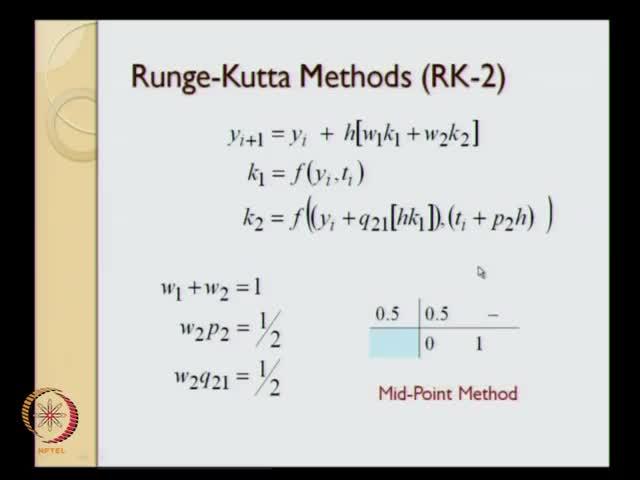
1 Computational Techniques Prof. Dr. Niket Kaisare Department of Chemical Engineering Indian Institute of Technology, Madras Module No. # 07 Lecture No. # 05 Ordinary Differential Equations (Refer Slide Time: 00:25) Hello and welcome to lecture 5 of module 7. We have been considering numerical methods for solving ordinary ordinary differential equations, the initial value problems in this particular module. So far we have covered the Runge-kutta family of method and specifically we have covered r k - 2 and r k - 4 methods. In the r k 2 method what what we do is, we write our y i plus 1 equal to y i plus h times slope, where slope is computed as some of two slopes k 1 and k 2. So, I will write this as h times w 1 k 1 plus w 2 k 2 that is the r k - 2 method, where k 1 is going to be equal to computed as the function f computed at (y i, t i), and k 2 is computed at some point y i plus q 2 multiplied by h k 1, t i plus p 2 multiplied by h what are sorry q2 2 1 multiplied by h k 1; this 2 corresponds to this particular 2 the same index, and this 1 index corresponds to this index 1 over here.

2 So, this is an explicit r k - 2 method that that we have over here. So, these weights w 1, w 2, q 2 1 and p 2 are related to each other based on certain rules, those rules were w 1 plus w 2 equal to 1; w 2 multiplied by q 2 1 equal to half; w 2 multiplied by p 2 equal to half. These were the three rules that we obtained; we have three equations for four unknowns, that means, one of those values we can choose on our on our own whichever value that we want, usually we tend to choose our value p 2. And based on that, we have looked at three different variants of r k - 2 method, the midpoint method, the Heun s method and the Ralston's method. So, this was about r k 2, and the way we represent these weights is, what we will do is will just draw a table with two lines, and the weights w 1 and w 2 will go below this this particular line, and the weights p at the weight p 2 will come to the left of the vertical line and q s we will write it in this particular row. So, we will have this q 2 1 over here and we would not have anything in this particular this particular column of the first row. So, this is going to be the representation for r k -2. Now, the r k - 4 method will have y i plus 1 computed as y i plus w 1 k 1 plus w 2 k 2 plus w 3 k 3 plus w 4 k 4, where k 1 was as before; k 2 was also as before the same expressions. We may not have the same q 2 1 and p 2 values, the expression is the same; it is not the values that are the same. k 3 is going to be equal to f of y i plus h multiplied by q 2 1 k 1 sorry q 3 1 k 1 this time plus q 3 2 k 2, t i plus p 3 multiplied by h; and k 4 is f of y i plus h multiplied by q 4 1 k 1 q 4 2 k 2 q 4 3 k 3. And now, we have our k 1, k 2, k 3 and k 4 for our r k - 4 method. And in r k - 4 method, the same kind of table will have w 1 w 2 w 3 and w 4 and then, instead of having just one row above this particular guy, we will have three rows above this guy- p 2 q 2 1, p 3 q 2 q 3 1 and q 3 2, and p 4 q and 4 3.

3 (Refer Slide Time: 06:00) (Refer Slide Time: 06:31)

4 (Refer Slide Time: 06:54) What I will do now is, I will go through some of the slides that I have already made, to show you some of the variants of the r k - 4 method, I will just go and review some of the things that we did in the last 5 minutes of the previous lecture and then, we will go on to the r k - 4 method. Let us start from essentially the over view of this particular module - in the r k family of method we have considered the r k - 2 and r k - 4 as higher order methods; r k 3 method is also there and usually its r k 2, r k 3 and r k - 4 methods that are typically more popular with r k - 4 being the most popular, and the reason for that is better ah accuracy of r k - 4 method compared to the any of the earlier methods. And the r k - 2 method, I had just written down on the board and I had gone over these particular expressions in in the previous lecture and we write this the weights in this particular form, q 2 2 the weight we are not going to use and so for different values of weights, we will get the midpoint method, the Heun s method and the Ralston's method.

5 (Refer Slide Time: 06:57) (Refer Slide Time: 07:33) Now, when we go to an r k n, we will have a general formulation of this type, where it is a weighted sum of k 1, k 2 up to k n, where k 1 is the slope computed at (y, t); k 2, k 3, k 4 and so on are the slopes computed at internal points. And we just on the green board, we just look at the expression that we get when n that is the number of internal points for computing the r k method was equal to 4 that is we have seen the r k - 4 variant on the green board of you a minute back. And the the table for r k - 4 method that we get will be constructed in this particular form.

6 So, we have the four weights w 1 w 2 w 3 and w 4; these are the weights for k 1 k 2 k 3 and k 4 to compute the slope S; p 2 p 3 and p 4 are the slopes in computing t i plus h multiplied by p; these are the p values, and q values are the weights that are computed are used in computing the intermediate y points using the r k method. For example, the classical r k method was p 2 was equal to half; p 3 was equal to half and p 4 was equal to 1, and q 2 1 was also equal to half.in And then, for computing k 3 we had we had used only k 2; we had not used k 1 at all. So, therefore, q 3 1 was 0; q 3 2 was half and p 3 was half. So, if you recollect what we did, was we computed the slope at the initial point, then we computed the slope at midpoint; midpoint means, the weights are going to be equal to half; we computed the slopes at midpoints using k 1, then we computed the slope again at midpoint not using k 1 that is why we get the 0, but using k 2, we computed the slope at the midpoint and that was called our k 3. And then, using the slope at k 3, we projected up to the end point so that is why this particular guy is equal to 1, because we are projecting up to end point, that means, we are projecting at t i plus 1 multiplied by h that is why this guy is 1; we did not use k 2 k 1 or k - 2 in this projection we only used k 3 in this projection. (Refer Slide Time: 10:07) So, it was y i plus h multiplied by k 3 and that is why we have this guy equal to 1; and the weights were 1 by 6; 2 by 6; 2 by 6 and 1 by 6. Remember that S, we computed as one sixth multiplied by k 1 plus 2 k 2 plus 2 k 3 plus k 4; so this is the classical Runge-

7 kutta fourth order method. Various different people have since device different methods for computing this for using this r k - 4 method. One of the more popular once explicit popular method is the Runge-kutta gills method. The reason why Runge-kutta gills method is popular, is the objective of the r k gill method is not just to minimize the truncation error, but it also tries to minimize the round off error. (Refer Slide Time: 10:43) So, with an objective function of minimizing the round off errors, these are basically the weights that are obtained for the r k gill method; perhaps is one of the most popular r k - 4 methods when it comes to non-adaptive r k - 4 methods. And finally, we have the Runge-kutta Fehlberg method; the Runge-kutta Fehlberg method comes under the category of embedded r k methods, and the embedded r k methods I will cover very briefly in the next lecture when I am going to discuss about in the next lecture when I discuss about the adaptive step size methods. And so, these are weights that are obtained for the Runge-kutta Fehlberg method. This is probably the most popular of the r k methods when we are going to use adaptive step size methods using what is known as this ah the types of r k methods. So, essentially what the weights that we get or of of this type, we have one fourth and one fourth weight for p and q, and these are the weights for computing k 3, and these are the weights for computing k 4, and once you get k 1 k 2 k 3 and k 4, these are the weights that you will use for w 1 w 2 w 3 and w 4. In fact you can actually indeed verify

8 that some w 1 w 2 w 3 plus w 4 is always going to be equal to 1 in all of the r k - 4 methods that we obtained. And this particular property that w 1 plus w 2 plus w 3 plus w 4 equal to 1 is required for consistency and we will talk about that in about ten minutes from now. (Refer Slide Time: 12:19) (Refer Slide Time: 12:33)

9 (Refer Slide Time: 12:46) So, now, to summarize what we get with the r k - 4 method what I have done is, I have used the solution using the r k - 4 method using the previous solver, that we had we had develop recall that we had developed this particular solver using the r k - 4 method and what I did was, I change h equal to 2.5, and for h equal to 2. 5 these are the results that we obtained for v equal to 0 v equal to 1; V equal to 0, V equal to 2. 5 and V equal to 5. (Refer Slide Time: 13:11) And for v going from V equal to 2. 5 to V equal to 5 what I have done is, I have just created an animation and I will just show that animation in the slide show, the dash line

10 that you see the purple thick dash that you see over here is the true solution; the three vertical lines that you see over here are t i, t i plus 1 and the midpoint. I have showed the midpoint, because in computing the classical r k - 4 method, we are going to use projections at the midpoint. So, we will start at this particular point and compute k 1. So, the k 1 is computed at the point shown by this black circle; so k 1 so the slope k 1 is just going to be equal to f of (y i, t i). So, the slope at this particular point will be k 1 and that is shown by the black line over here and then, we project along this slope up to the midpoint to compute our k 2. Keep in mind, the k 2 was computed at f of i plus half for time t, and i plus k 1 h by 2 for y i. So, k 2 is going to be computed at this point; it is computed at (t i, y i). So, the k 2 computed at this point these are actual slopes that are obtained from from excel. This is not a cartoon; these are indeed actual slopes that I have obtained from excel and I have animated the slope. So, this particular red line that you see over here is the slope k 2, and using the slope k 2, we are going to project to project over here in order to get our k 3; k 3 again is obtained at the midpoint. So, we take this particular arrow, this slope is unchanged and we will just bring it back to the point (t i, y i) and then, project it to the midpoint. So, the t point (t i, y i) is projected at the midpoint and that we will get as k 3, and the k 3 is f computed at y i plus k 2 h by 2 that is this particular point, and t i plus h by 2, which is this vertical point over here. Now, k 3 will be computed at this point and the k 3 that is computed at this point is shown by the blue arrow over here. So, this red arrow sorry the black arrow is k 1; this red arrow is k 2; this blue arrow is k 3, and the blue arrow gets again moved back to the point (y i, t i). And now, what we are going to do is, we are going to use k 3 to project at t i plus 1. So, we will project along this line all the way up to t i plus 1 and will compute the slope at that point t i plus 1.

11 (Refer Slide Time: 16:38) So, this is the point at which we will compute our fourth slope, which will be given by this green line. So, this is the slope computed at this particular guy k 4 computed at i plus 1 for the time, and i plus h times k 3 for the concentration. So, this is the green slope representing k 4 and we now take this green slope back over here. So, now, we have k 1, k 2, k 3 and k 4; I have discarded all those lines for lines for projections. So, 1 multiplied by k 1 plus 2 multiplied by by k 2 plus 2 multiplied by k 3 plus 1 multiplied by k 4; the entire thing divided by 6 is going to give us the final slope S and using that final slope, we will project up to from this point, we will end up reaching actually the point right over here. So, this is geometric interpretation of r k - 4 method using the actual values for r k the classical r k - 4 from the Microsoft excel.

12 (Refer Slide Time: 17:27) (Refer Slide Time: 17:37) We will do the same thing for Heun s method also. If we go on to some of the earlier slide, I will just go on to the the overview slide; we have covered the Heun s method under the context of higher order Runge-kutta method. Now, what I will do is I will go on to the predictor-corrector methods and I will give you a motivation for using the Heun s using the Heun s method, I will motivate the predictor-corrector methods. So, the Heun s method variant, the r k - 2 variant of Heun s method is, k 1 is the slope computed at this point and we project all the way up to y i all the way up to t i plus 1. So,

13 for the k 2 will be the slope computed at y plus h times k 1 and t i plus 1. So, t i plus h is t i plus 1; y i plus h times k 1 is what we will call as y bar. So, the r k - 2 variant is y i plus 1 equal to y i plus h by 2 multiplied by k 1 plus k 2. Now, what we can say about k 1, is that k 1 predicts, what value we will reach with y i plus 1; so this y bar i plus 1 is the predicted value y i plus 1. (Refer Slide Time: 19:33) So, what we are going to say in the predictor-corrector form is, instead of calling this as y i plus 1 equal to y i plus h by 2 times k 1 plus k 2, we will call this as y i plus 1 equal to y i plus h by 2 times f of (y i, t i) plus f of (y bar i plus 1, t i plus 1), where y bar is the predicted value, y i plus h times k 1 so this is the predictor-corrector variant. Now, let us put the Heun s method in the predictor-corrector form. So, k 1 is the slope computed over here; y i y i plus 1 bar 0 is the predicted point at this particular location. And now, we write in the corrector equations, the corrector equation is k 2 0 is going to be nothing but f at y i plus 1 bar 0, t i plus 1, and the new value y bar i plus 1 computed using the first iteration is going to be y i plus h by 2 multiplied by k 1 plus k 2. So, if we stop at this location what we are going to get is, we are going to have these two slopes - this black slope and this red slope and the new slope is going to be just an average of the slope using the Heun s method. If we stop at this point, we will get a predictor-corrector form of Heun s method, which is exactly the same as the r k - 2 method, but there is no need to stop at this point. This is

14 going to be the average of the two slopes; the average of the red line over here and the black line over here is shown by this particular thin line. Now, this thin line with we can use to project once again to get y bar i plus 1 2; this y bar i plus 1 1 in the same manner we can get y bar i plus 1 2, which is essentially going to be this point. Keep in mind k 2 m is just going to be nothing but this particular slope, which is midpoint of though of the previous slopes. And now, we compute the slope at this point, we projected back that the slope computed at this point discard the red lines, which represent the the corrector forms for the first iteration. So, now, we have the corrector form for the second iteration; now, we have this black line and this blue line and we can get the average of the black and blue line and we can keep repeating this again and again multiple number of times in order to get the Heun s method the predictor-corrector form. So, what I have done is, I have shown you the Heun s method in the predictor-corrector forms using animation using Microsoft excel results. Now, what I will do is, I will go on to the green board and I will again re-derive the Heun s method using the predictorcorrector form. (Refer Slide Time: 22:16) So, now, let us on the on the green board, let us see the r k - 2 variant of Heun s method and then, the predictor predictor-corrector variant of Heun s method. The general r k - 2 method had already written written down on the board. For Heun s method, the weights

15 w 1 and w 2 are 1 by 2 and 1 by 2; so I will replace them by that those numbers. So, I will replace w 1 and w 2 by half each and I will take half outside the bracket; so will get this as h by 2. k 1 was nothing but f computed at (y i, t i )and k 2 is f computed at y i plus 1 multiplied by h k 1 that was what Heun s method was. Our q 2 1 and our p 2, were both equal to 1. So, I will write it in that particular form; so it is h multiplied by k 1 and t i plus h over here; so this is going to be our k 2. Now, what we do is, we call this particular guy, we call this as a predicted value will call this predicted value y bar i plus 1 0, and this predicted value we will correct it using Heun s method recursively. So that is what we are we are going to do with with this. Now, here if we were to use this r k - 2 variant, this is where we stop and we do not proceed ahead any further this becomes the r k - 2 variant, which is equivalent to the Heun s method predictor-corrector with the corrector used once only. (Refer Slide Time: 24:17)

16 (Refer Slide Time: 24:49) Now, the predictor-corrector form of Heun s method, where we use the predictorcorrector multiple time is what I am going to write now. So, the Heun s method with the predictor-corrector form, again we will we will write down the same expressions, pretty much will derive the same expressions in the same form. First thing to do is to derive the predicted value. So, first item in our agenda is to choose the predictor, which uses the value k 1 only. So, our predicted value y i plus 1 bar 0 is going to be equal to y i plus h multiplied by f of (y i, t i). So, if we look at what our y i bar 0 was, if we go back to this particular part and see what our y i bar 0 was, y i bar 0 was nothing but y i plus h times k 1; k 1 was nothing but f of (y i, t i) that is the predictor that so that is the same equation that I have written in a slightly different form over here. Now, let us look at the corrector form of the equation. Corrector is nothing but a trapezoidal rule that we use. Two lectures earlier, I believe in lecture 3, we had shown that the Heun s method is kind of like using a trapezoidal rule, if we had the function f as function just of the time t; likewise, the corrector form is going to be the implementation of trapezoidal rule. In the corrector form what we do is y i plus 1 corrected, we will write this equal to y i plus h by 2 multiplied by k 1 plus k 2. We have this as k in in computing The Heun s method using r k - 2 we have y i plus 1 equal to y i plus h by 2 multiplied by k 1 plus k 2 what is k 1? k 1 is nothing but the slope

17 computed at y i t i. What is k 2? k 2 is nothing but slope computed at y i plus 1 bar 0 and t i plus 1. So, I will write that down over here; so h by 2 multiplied by f of (y i, t i) plus f at y i plus 1 bar 0, t i plus 1. Now, if we stop at this point, the result that we get from the Heun s predictor-corrector method is the same as the result that we will get from the r k - 2 method, but we are not going to stop at this point, but we will going to use the corrector multiple number of times. So, the third item is the multiple use of corrector. (Refer Slide Time: 28:13) So, what do you mean by multiple use of corrector? Instead of calling this as just y i plus 1 corrected, I will just erase this corrected part; I will put a bar over here and write this as y bar i plus 1 superscript 1. So, the multiple uses of corrector would be y i plus 1 bar 2 is going to be equal to y i plus h by 2 multiplied by f of (y i, t i) plus f of (y i plus 1 bar 1, t i plus 1). So, if we compare it with the first use of corrector, if we compare the second use of corrector, instead of computing y i plus 1 bar 1, we are now computing y i plus 1 bar 2. This guy remains the same; this particular guy does not change what it means? It means, it is the slope that is computed at the initial point. So, this means it is a slope computed over here. y bar 0 is going to be y bar i plus 1 0 is going to be the point that is projected using this particular slope. So, yi y bar 0 is going to be the yellow line; that so y bar 0 is the point by the yellow x, and f of y bar 0 is going to be the yellow arrow over here.

18 So, now, what what we do with with this particular guy is that we project again using the average slope of y bar 1 and y i. So that means, we are going to use this yellow slope and this white slope and then, we will get this is a average slope is going to lie midway between these two arrows and that is going to be this particular dotted line. So, our x over here or the star over here is going to be this particular guy over there. And the slope computed at that point is I am going to show this with a red arrow, and that red arrow is going to be the slope computed over here and that red arrow is this this particular guy and then, I will get I will draw this red arrow over here. I will now discard this yellow arrows; I do not really need these yellow arrows any more so I will just discard this yellow arrows get an average slope of this white and this red arrow and that white average slope I am going to predict once again to the end and this is our purple x ; our purple x is over here. Now I can use So, this is the second time I have used the corrector; I will use the corrector third time, fourth time and so on and so forth. I will use it recursively in order to get better and better guesses. So, the recursive use of this corrector means that this guy has to be replaced by appropriate quantity. (Refer Slide Time: 31:54) So, we will replace this with m plus 1 equal to y i plus h by 2 f y i t i plus f of y i bar m, instead of (1, t i), where y 0 is obtained from this particular equation and this equation is

19 used for m equal to 0 to some M. So, we use this predictor the corrector equation a capital M number of times, lets we predecide what this M is going to be. So, let us say that we are going to use the corrector equation five times. So, we will use the predictor equation once; we will use y y 0 in order to compute y bar 1; y bar 1 we will use to compute y bar 2; y bar 2 to y bar 3; y bar 3 to y bar 4; and y bar by 4 to compute y bar 5, when when we reach y bar 5 that is what we say that the solution is the solution that we need for d i plus 1 and entire process is repeated all over again at the next step. So that is the idea behind predictor-corrector methods. We will take up predictorcorrector methods once again in the last lecture of this module when we are when I very briefly I am going to cover some of the more advanced methods and why this idea of predictor-corrector method actually is fairly popular and some of these methods, specifically in the Adam-Moulton family of methods, those are also the predictorcorrector methods. So, in summary what we have covered so far is, we have covered r k methods; we have covered the error analysis of r k methods and we have covered the predictor-corrector methods. The error analysis of the predictor-corrector methods is fairly straight forward; this is nothing but an Euler s explicit method. As a result, the error for the predictor equation is that its order of h squared, whereas the corrector equation is kind of like using the trapezoidal method and because it is kind of like using the trapezoidal method, the error in corrector equation is of the order of h cubed. So, this this error is of the order of h cube; this error is of the order of h squared. Now, why is this particular method actually useful? The reason why predictor-corrector methods are useful is because they are still explicit methods; they are not implicit method. But if this Heun s method was repeated large enough number of times, in that case what will happen is that if there is convergence, then Heun s method will converge to a totally an implicit method. Why that is so? is What what I mean by that is every time what we do is when we use this particular equation y i, y bar m plus 1 is changing compared to y bar m plus m.

20 (Refer Slide Time: 35:33) So, if we go from y bar 0 to y bar 1 and so on up to say y bar m and we go to y bar m plus 1, if the error between y bar m and y bar m plus 1 is very small if that error is very small, then if we are going to substitute that in this particular equation. The equation that we are going to get is y bar m plus 1 is going to be equal to y i plus h by 2 multiplied by f of (y i, t i) plus f of y bar m i plus 1, t i plus 1. If m is large enough, we repeat this multiple number of times till we get convergence. If m if m is large enough for convergence, then what what what we are going we are saying is y bar m plus 1is approximately equal to y bar m and let us just represent this as y m or let just represent as y bar without any superscript over here. So, if we write if we write y bar m plus 1 equal to y bar, and y bar m also equal to y bar we will get our y bar computed at time i plus 1 equal to y i plus h by 2 multiplied by f of (y i, t i) plus f of (y i plus 1 bar, t i); keep in mind that this bar just represents a dummy type of variable.

21 (Refer Slide Time: 38:53) Now, if you see this particular equation, this equation is if you recollect something that we did in lecture two of this particular module, this is nothing but Crank-Nicholson method. And this completes the promise that I made in the in lecture in lecture 2 itself, why Crank-Nicholson method is going to be preferred over implicit Euler method. The reason why Crank-Nicholson method is going to be preferred over implicit Euler method is because implicit Euler method we derive were we saw was of the order of h square accurate and we have just derived that. Because of this corrector equation, a method of the type of Crank-Nicholson method is h cube accurate. So, to recollect what we have done in the last half an hour - we started with r k - 2 method, specifically we started with the Heun s variant of the of the r k - 2 method. From the r k - 2 method we said that by repeatedly calculating this guy k 2, what we are going to do is, we are going to convert that r k - 2 method into a predictor-corrector Heun s method.

22 (Refer Slide Time: 39:07) (Refer Slide Time: 39:25) In the Heun s method, we use this predictor equation that means we use k 1 as a predictor equation and then, use the k 2 equation repeatedly in order to improve or in order to correct the value of y bar. If you go from y bar 0 to y bar 1 and so on up to y bar capital M. So, this what we do in order to use the predictor-corrector Heun s method.

23 (Refer Slide Time: 40:01) Now, instead of stopping at capital M number of iterations, if we keep doing the iterations, until y bar m plus 1 converges to y bar m, then what we have solved over here is, we have essentially solved a non-linear equation of this type. We have solved this equation using the fixed-point iteration method - the method of successive evaluations. So, if we actually do that, we will get Crank-Nicholson method. If we stop at a finite number of iterations, we will get the predictor-corrector method; if we stop only in the first step, not do any iterations of the corrector, we will get the r k - 2 Heun s method. So that is basically what I wanted to cover with of respect to r k - 2 methods and with respect to the predictor-corrector methods.

24 (Refer Slide Time: 41:36) The next question and a very important question comes up is why do you want to look at the implicit methods at the at the first in the first case itself? Because the the r k - 2 method we saw had an accuracy of h cubed; predictor-corrector had an accuracy of h cube; Crank-Nicholson method has as accuracy of h cube, but clearly the amount of effort that is required in order to solve this particular algebraic equation problem is significantly higher than the amount of effort that is required to solve the r k the r k - 2 method. So, the question comes is why implicit method and the answer to that question is because implicit methods are more stable. The question is what do we mean by a stability?

25 (Refer Slide Time: 42:04) So, let us again go back to the Microsoft excel and try to see what we actually mean by stability. Now, let us consider what we mean by stability and what I have done over here is from the same excel sheet that we have we have been looking at in the in the past few lectures, I have opened up the same Euler s explicit method sheet. So, this is where we computed the ah we where we used Euler s explicit method in order to compute the solution for V equal to 5, given that concentration C 0 equal to 1. What we had seen is, as we decrease the value of our step size h, we get more and more accurate results; likewise, as we increase the value of our step size, we are going to get less and less accurate results.

26 (Refer Slide Time: 43:02) So, from h equal to 1, let me increase this to h equal to 1.5, what happens when we increase this to h equal to 1.5? What I will do is I will just take this figure a little bit away so that they do not distract us from our discussion. (Refer Slide Time: 43:33) So, what happens when we go from h equal to 1 to h equal to 1. 5 is that the error that we get increases, but nothing more has happened, besides error increasing. Let us go to h equal to 1. 8 and again, we find that the error has increased even further.

27 (Refer Slide Time: 43:42) Let us now go to h equal to 2; now, when we see h equal to 2, there is some funny business that is happening. Let If we look at the predictions of the Euler s method with h equal to 2, the initial concentration was equal to 1, but the concentration immediately at volume V equal to 2 has dropped to 0, and beyond that, this method cannot continue because C itself is 0; when C is 0, f that is computed is 0; if f that is computed is 0, then C i plus 1 equal to C plus h multiplied by f is going to be equal to C i itself. So, C i plus 1 equal to C i equal to 0. So, immediately within one step C i c I has gone to a value equal to 0. (Refer Slide Time: 44:49)

28 So, now, that is a little bit of a problem over here. This problem arises, because at h equal to 2, we have limit of stability of this particular method what that means is lets go from h equal to 2 to h equal to And if we go to h equal to 2 to h equal to 2.1, this is what we observe. What we observe is quite clearly that the concentration goes to a negative value and beyond that our method cannot cannot proceed. The reason why the method cannot proceed is because the concentration to the power , it is a fractional power. As a result of the fractional power, because we get negative concentration; we are not able to proceed further. (Refer Slide Time: 45:37) So, now, what I will do is, I will change this problem a little bit from d C by d V equal to to d C by d V equal to minus C to the power 1 divided by 2. And what what we will do is, we will go back to h equal to 0. 5, and let us see what happens now. Let us consider the case, where we have f to the power 1, instead of f to the power , everything else remains the same; I have only changed this particular expression over here. So, now, I will drag it and drop it over here and the true values are also going to change. True values is are going to be F or the first order reaction, the basically the true values are going to be e to the power minus t by 2 or e into minus 2 t. So, with with this particular change we what we have is d C by d V; d C by d V is going to be equal to minus 0. 5 into C.

29 So, what we can do is, d C we can write this as d C divided by C is going to be equal to minus 0. 5 into d V and when we integrate this, we are going to get l n of C equal to minus 0. 5 into v integrating from 0 to v and from C A 0 to C A. So, we will have l n of C A C divided by C A 0, where C A 0 was equal to 1. So, l n of C by C is going to be equal to minus 0. 5 V or C is going to be e to the power minus 0. 5 and this is what we have written over here, concentration is equal to e to the power minus 0. 5 multiplied by V or minus V divided by 2 so that is the true value that we get. The numerical value using Euler s explicit method for h equal to 0. 5 or as shown over here and we can extended further. (Refer Slide Time: 49:06) And we can extend it up to V equal to 5 and we will get the concentration of the species coming out from the PFR using the Euler s explicit method. Now, let us increase our h to 1 and see what happens. When our h has increased to 1, the overall errors have also increased. So, the errors have increased, indeed when we have we go from h equal to. 5 2 h equal to 1, but the solution is still available for us to see.

30 (Refer Slide Time: 49:27) Now, for if we go from h equal to 1 to h equal to 2 what happens is what we had seen earlier; immediately the concentration has becomes 0 and from that point onwards, we cannot proceed. (Refer Slide Time: 49:42) Now, what do we do, if h happens to be h equal to 2. 1? And this is what we see when h equal to 2. 1 is that the concentration has become 1, has become negative and then, it is oscillating and finally, settling down at the steady state value.

31 (Refer Slide Time: 50:02) (Refer Slide Time: 50:12)

32 (Refer Slide Time: 50:23) Now, let us say if h equal to 4 what happens. We get the value oscillating at 1, minus 1, 1, minus 1, 1 minus 1 and so on. Now, if h is increased to 5, there is an interesting thing that happens. It is 1, minus 1.5, 2, minus 3, 5, minus 7. Now, when I increase h to 10 see what is happening is, see 1, minus 4, 16, minus 64, 256, So, what essentially is happening over here is as we are increasing h beyond a certain point, the solution from Euler s method is going unstable. So, I will go to the green board and I will plot out what actually happened in the Euler s explicit method. (Refer Slide Time: 51:00)

33 So, what I have said over here is implicit methods are more stable; we are investigating what it means by stability. So, what happened what we saw over here is we were if we were to plot the concentration C against the volume, the the numerical method for getting concentration C against the volume, if we were to use say h equal to 1, we will perhaps get the results something like this. If we were to use h equal to 2, we will get perhaps the result going something like this; when we used when we used value h equal to 2.1, the results that we got were something of this sort; this is with when h again this this is a cartoon. So, this not exactly drawn with scale; this is just to show you what what we get. (Refer Slide Time: 52:28) Now, when h was equal to 4, the type of results that we got when h was equal to 4. So, this we started out at 1; this value was minus 1; this value again was 1; this value was minus 1; this was 1 and this value was minus 1 again. So, this is the curve that we got when h was equal to 4. Now, what do we get when h increased is increased to beyond 4? What we get when h is increased to beyond 4 is this particular value goes beyond minus 1, the next value goes beyond 1, the value after that goes even below minus 1 so on and so forth. So, if we were to shrink this plot, we were if we were to shrink the the ordinate for this particular system and we were to plot this for h greater than 4, we will start at minus 1 sorry we will start at plus 1; go to a value below minus 1 and if we repeat it for large enough volume what we will get is, we will get the overall result oscillating between minus infinity and plus infinity as re-tends to infinity. This is known as an unstable solution. So, I am going to end the lecture over here in this in the lecture 5 of this module. I am going to end over here.

34 (Refer Slide Time: 54:46) In the next lecture, I am going to consider the stability issues; specifically I will talk about the equation. So, the equation that we had d C by d V was equal to minus C by 2. For this particular condition, we saw that when h becomes greater than 4, at that time the explicit Euler s method becomes unstable. And we will do some theoretical analysis of this particular condition to find out under what conditions do the explicit Euler s method becomes unstable, under what conditions do the implicit Euler method methods become unstable. And what we will show is that implicit methods are globally stable; there is no limit on h for which this remains unstable. What we will also show is that for the condition for which explicit Euler s method becomes stable is going to be, when h is greater than 2 divided by the coefficient of this term. When that h is greater than 2 divided by 1 by 2 that is where the explicit Euler s method is going to be unstable, that is something that we are going to start off in the next lecture in this particular module. Thank you.