3.4. A computer ANOVA output is shown below. Fill in the blanks. You may give bounds on the P-value.

Transcription

1 3.4. A computer ANOVA output is shown below. Fill in the blanks. You may give bounds on the P-value. One-way ANOVA Source DF SS MS F P Factor ??? Error??? Total Completed table is: One-way ANOVA Source DF SS MS F P Factor Error Total

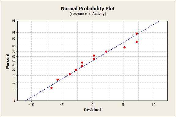
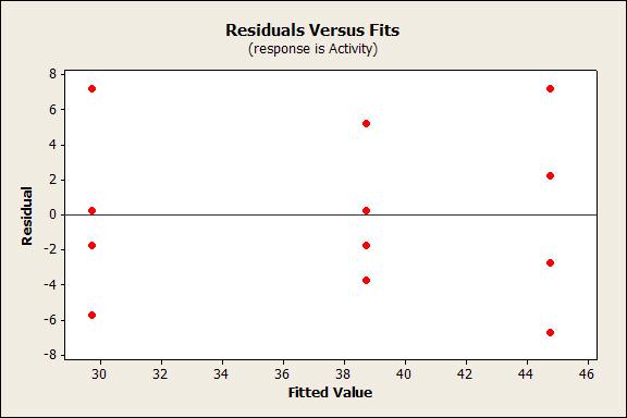
2 3.11. A pharmaceutical manufacturer wants to investigate the bioactivity of a new drug. A completely randomized single-factor experiment was conducted with three dosage levels, and the following results were obtained. Dosage Observations 20g g g (a) Is there evidence to indicate that dosage level affects bioactivity? Use = Minitab Output One-way ANOVA: Activity versus Dosage Analysis of Variance for Activity Source DF SS MS F P Dosage Error Total There appears to be a difference in the dosages. (b) If it is appropriate to do so, make comparisons between the pairs of means. What conclusions can you draw? Because there appears to be a difference in the dosages, the comparison of means is appropriate. Minitab Output Tukey 95% Simultaneous Confidence Intervals All Pairwise Comparisons among Levels of Dosage Individual confidence level = 97.91% Dosage = 20g subtracted from: Dosage Lower Center Upper g ( * ) 40g ( * ) Dosage = 30g subtracted from: Dosage Lower Center Upper g ( * ) The Tukey comparison shows a difference in the means between the 20g and the 40g dosages. (c) Analyze the residuals from this experiment and comment on the model adequacy. There is nothing too unusual about the residual plots shown below.

3

4 5.1. The following output was obtained from a computer program that performed a two-factor ANOVA on a factorial experiment. Two-way ANOVA: y versus A, B Source DF SS MS F P A 1? ?? B? ??? Interaction ?? Error ? Total (a) Fill in the blanks in the ANOVA table. You can use bounds on the P-values. Two-way ANOVA: y versus A, B Source DF SS MS F P A B Interaction Error Total (a) How many levels were used for factor B? 4 levels. (b) How many replicates of the experiment were performed? 2 replicates. (c) What conclusions would you draw about this experiment? Factor B is moderately significant with a P-value of Factor A and the two-factor interaction are not significant.

5 5.4. A mechanical engineer is studying the thrust force developed by a drill press. He suspects that the drilling speed and the feed rate of the material are the most important factors. He selects four feed rates and uses a high and low drill speed chosen to represent the extreme operating conditions. He obtains the following results. Analyze the data and draw conclusions. Use = (A) Feed Rate (B) Drill Speed Response 1 Force ANOVA for selected factorial model Analysis of variance table [Classical sum of squares - Type II] Sum of Mean F p-value Source Squares df Square Value Prob > F Model significant A-Drill Speed B-Feed Rate AB Pure Error E-003 Cor Total The Model F-value of implies the model is significant. There is only a 0.07% chance that a "Model F-Value" this large could occur due to noise. Values of "Prob > F" less than indicate model terms are significant. In this case A, B, AB are significant model terms. The factors speed and feed rate, as well as the interaction is important. Design-Expert Software Force Design Points A1 Level 1 of A A2 Level 2 of A Interaction A: Drill Speed X1 = B: Feed Rate X2 = A: Drill Speed Force Level 1 of B Level 2 of B Level 3 of B Level 4 of B B: Feed Rate The standard analysis of variance treats all design factors as if they were qualitative. In this case, both factors are quantitative, so some further analysis can be performed. In Section 5.5, we show how response curves and surfaces can be fit to the data from a factorial experiment with at least one quantative factor. Since both factors

6 in this problem are quantitative, we can fit polynomial effects of both speed and feed rate, exactly as in Example 5.5 in the text. The Design-Expert output with only the significant terms retained, including the response surface plots, now follows. Response 1 Force ANOVA for Response Surface Reduced Quadratic Model Analysis of variance table [Partial sum of squares - Type III] Sum of Mean F p-value Source Squares df Square Value Prob > F Model significant A-Drill Speed B-Feed Rate B Residual E-003 Lack of Fit significant Pure Error E-003 Cor Total The Model F-value of implies the model is significant. There is only a 0.11% chance that a "Model F-Value" this large could occur due to noise. Values of "Prob > F" less than indicate model terms are significant. In this case A, B 2 are significant model terms. Std. Dev R-Squared Mean 2.77 Adj R-Squared C.V. % 3.00 Pred R-Squared PRESS 0.14 Adeq Precision Coefficient Standard 95% CI 95% CI Factor Estimate df Error Low High VIF Intercept A-Drill Speed B-Feed Rate B Final Equation in Terms of Coded Factors: Force= * A * B +0.13* B 2 Final Equation in Terms of Actual Factors: Force = E-003 * Drill Speed * Feed Rate

7 Force B: Feed Rate A: Drill Speed Design-Expert Software Force Design points above predicted value Design points below predicted value X1 = A: Drill Speed X2 = B: Feed Rate Force B: Feed Rate A: Drill Speed

8 6.2. An engineer is interested in the effects of cutting speed (A), tool geometry (B), and cutting angle on the life (in hours) of a machine tool. Two levels of each factor are chosen, and three replicates of a 2 3 factorial design are run. The results are as follows: Treatment Replicate A B C Combination I II III (1) a b ab c ac bc abc (a) Estimate the factor effects. Which effects appear to be large? From the normal probability plot of effects below, factors B, C, and the AC interaction appear to be significant. DESIGN-EXPERT Plot Life Normal plot A: Cutting Speed B: Tool Geometry C: Cutting Angle Normal % probability A C B 1 AC Effect (b) Use the analysis of variance to confirm your conclusions for part (a). The analysis of variance confirms the significance of factors B, C, and the AC interaction. Response: Life in hours ANOVA for Selected Factorial Model Analysis of variance table [Partial sum of squares] Sum of Mean F Source Squares DF Square Value Prob > F Model significant A B C AB AC BC ABC Pure Error Cor Total

9 The Model F-value of 7.64 implies the model is significant. There is only a 0.04% chance that a "Model F-Value" this large could occur due to noise. The reduced model ANOVA is shown below. Factor A was included to maintain hierarchy. Response: Life in hours ANOVA for Selected Factorial Model Analysis of variance table [Partial sum of squares] Sum of Mean F Source Squares DF Square Value Prob > F Model < significant A B < C AC Residual Lack of Fit not significant Pure Error Cor Total The Model F-value of implies the model is significant. There is only a 0.01% chance that a "Model F-Value" this large could occur due to noise. Effects B, C and AC are significant at 1%. (c) Write down a regression model for predicting tool life (in hours) based on the results of this experiment. y x x x x ijk A B C A x C Coefficient Standard 95% CI 95% CI Factor Estimate DF Error Low High VIF Intercept A-Cutting Speed B-Tool Geometry C-Cutting Angle AC Final Equation in Terms of Coded Factors: Life = * A * B * C * A * C Final Equation in Terms of Actual Factors: Life = * Cutting Speed * Tool Geometry * Cutting Angle * Cutting Speed * Cutting Angle The equation in part (c) and in the given in the computer output form a hierarchial model, that is, if an interaction is included in the model, then all of the main effects referenced in the interaction are also included in the model. (d) Analyze the residuals. Are there any obvious problems?

10 Normal plot of residuals Residuals vs. Predicted Normal % probability Residuals Residual Predicted There is nothing unusual about the residual plots. (e) Based on the analysis of main effects and interaction plots, what levels of A, B, and C would you recommend using? Since B has a positive effect, set B at the high level to increase life. The AC interaction plot reveals that life would be maximized with C at the high level and A at the low level. DESIGN-EXPERT Plot Life 60 Interaction Graph Cutting Angle DESIGN-EXPERT Plot Life 60 One Factor Plot X = A: Cutting Speed Y = C: Cutting Angle 50.5 C C Actual Factor B: Tool Geometry = Life X = B: Tool Geometry Actual Factors A: Cutting Speed = 0.00 C: Cutting Angle = 0.00 Life Cutting Speed Tool Geometry

11 6.12. A nickel-titanium alloy is used to make components for jet turbine aircraft engines. Cracking is a potentially serious problem in the final part, as it can lead to non-recoverable failure. A test is run at the parts producer to determine the effects of four factors on cracks. The four factors are pouring temperature (A), titanium content (B), heat treatment method (C), and the amount of grain refiner used (D). Two replicated of a 2 4 design are run, and the length of crack (in m) induced in a sample coupon subjected to a standard test is measured. The data are shown below: Treatment Replicate Replicate A B C D Combination I II (1) a b ab c ac bc abc d ad bd abd cd acd bcd abcd (a) Estimate the factor effects. Which factors appear to be large? From the half normal plot of effects shown below, factors A, B, C, D, AB, AC, and ABC appear to be large. Term Effect SumSqr % Contribtn Model Intercept Model A Model B Model C Model D Model AB Model AC Error AD Error BC Error BD Error CD Model ABC Error ABD Error ACD Error BCD Error ABCD

12 DESIGN-EXPERT Plot Crack Length Half Normal plot A: Pour Temp B: Titanium Content C: Heat Treat Method D: Grain Ref iner AC 95 B Half Normal %probability BC D AB C ABC A Effect (b) Conduct an analysis of variance. Do any of the factors affect cracking? Use =0.05. The Design Expert output below identifies factors A, B, C, D, AB, AC, and ABC as significant. Response: Crack Lengthin mm x 10^-2 ANOVA for Selected Factorial Model Analysis of variance table [Partial sum of squares] Sum of Mean F Source Squares DF Square Value Prob > F Model < significant A < B < C < D < AB < AC < AD BC BD CD ABC < ABD ACD 2.926E E BCD ABCD 1.596E E Residual Lack of Fit Pure Error Cor Total The Model F-value of implies the model is significant. There is only a 0.01% chance that a "Model F-Value" this large could occur due to noise. Values of "Prob > F" less than indicate model terms are significant. In this case A, B, C, D, AB, AC, ABC are significant model terms. (c) Write down a regression model that can be used to predict crack length as a function of the significant main effects and interactions you have identified in part (b). Final Equation in Terms of Coded Factors: Crack Length= *A

13 +1.99 *B *C *D *A*B *A*C * A * B * C (d) Analyze the residuals from this experiment. Normal plot of residuals Residuals vs. Predicted Normal % probability Residuals Residual Predicted There is nothing unusual about the residuals. (e) Is there an indication that any of the factors affect the variability in cracking? By calculating the range of the two readings in each cell, we can also evaluate the effects of the factors on variation. The following is the normal probability plot of effects: DESIGN-EXPERT Plot Range Normal plot A: Pour Temp B: Titanium Content C: Heat Treat Method D: Grain Refiner Norm al % probability AB CD Effect It appears that the AB and CD interactions could be significant. The following is the ANOVA for the range data:

14 Response: Range ANOVA for Selected Factorial Model Analysis of variance table [Partial sum of squares] Sum of Mean F Source Squares DF Square Value Prob > F Model significant AB CD Residual Cor Total The Model F-value of implies the model is significant. There is only a 0.14% chance that a "Model F-Value" this large could occur due to noise. Values of "Prob > F" less than indicate model terms are significant. In this case AB, CD are significant model terms. Final Equation in Terms of Coded Factors: Range = * A * B * C * D (f) What recommendations would you make regarding process operations? Use interaction and/or main effect plots to assist in drawing conclusions. From the interaction plots, choose A at the high level and B at the low level. In each of these plots, D can be at either level. From the main effects plot of C, choose C at the high level. Based on the range analysis, with C at the high level, D should be set at the low level. From the analysis of the crack length data: DESIGN-EXPERT Plot Crack Length Interaction Graph B: Titanium Content DESIGN-EXPERT Plot Crack Length Interaction Graph C: Heat Treat Method X = A: Pour Temp Y = B: Titanium Content X = A: Pour Temp Y = C: Heat Treat Method B B Actual Factors C: Heat Treat Method = 1 D: Grain Refiner = Crack Length C1-1 C2 1 Actual Factors B: Titanium Content = 0.00 D: Grain Refiner = Crack Length A: Pour Tem p A: Pour Tem p

15 DESIGN-EXPERT Plot Crack Length X = D: Grain Refiner One Factor Plot DESIGN-EXPERT Plot Crack Length X = A: Pour Temp Y = B: Titanium Content Z = C: Heat Treat Method Cube Graph Crack Length Actual Factors A: Pour Temp = 0.00 B: Titanium Content = 0.00 C: Heat Treat Method = 1 Crack Length Actual Factor D: Grain Refiner = 0.00 B: Titanium Content B C+ C: Heat Treat Metho B C- A- A+ A: Pour Tem p D: Grain Refiner From the analysis of the ranges: DESIGN-EXPERT Plot Range Interaction Graph B: Titanium Content DESIGN-EXPERT Plot Range Interaction Graph D: Grain Refiner X = A: Pour Temp Y = B: Titanium Content X = C: Heat Treat Method Y = D: Grain Refiner B B Actual Factors C: Heat Treat Method = 0.00 D: Grain Refiner = Range D D Actual Factors A: Pour Temp = 0.00 B: Titanium Content = Range A: Pour Tem p C: Heat Treat Method

16 7.2 Consider the experiment described in Problem 6.2. Analyze this experiment assuming that each replicate represents a block of a single production shift. Source of Sum of Degrees of Mean Variation Squares Freedom Square F 0 Cutting Speed (A) <1 Tool Geometry (B) * Cutting Angle (C) * AB <1 AC * BC ABC <1 Blocks Error Total Response: Life in hours ANOVA for Selected Factorial Model Analysis of variance table [Partial sum of squares] Sum of Mean F Source Squares DF Square Value Prob > F Block Model significant A B C AC Residual Cor Total The Model F-value of implies the model is significant. There is only a 0.01% chance that a "Model F-Value" this large could occur due to noise. Values of "Prob > F" less than indicate model terms are significant. In this case B, C, AC are significant model terms. These results agree with the results from Problem 6.2. Tool geometry, cutting angle and the interaction between cutting speed and cutting angle are significant at the 5% level. The Design Expert program also includes factor A, cutting speed, in the model to preserve hierarchy.

17 7.3. Consider the data from the first replicate of Problem 6.2. Suppose that these observations could not all be run using the same bar stock. Set up a design to run these observations in two blocks of four observations each with ABC confounded. Analyze the data. Block 1 Block 2 (1) a ab b ac c bc abc From the normal probability plot of effects, B, C, and the AC interaction are significant. Factor A was included in the analysis of variance to preserve hierarchy. DESIGN-EXPERT Plot Life Normal plot A: Cutting Speed B: Tool Geometry C: Cutting Angle B Norm al % probability AC C Effect Response: Life in hours ANOVA for Selected Factorial Model Analysis of variance table [Partial sum of squares] Sum of Mean F Source Squares DF Square Value Prob > F Block Model not significant A B C AC Residual Cor Total The "Model F-value" of 7.32 implies the model is not significant relative to the noise % chance that a "Model F-value" this large could occur due to noise. There is a Values of "Prob > F" less than indicate model terms are significant. In this case there are no significant model terms. This design identifies the same significant factors as Problem 6.2.

18 8.3. Suppose that in Problem 6.12, only a one-half fraction of the 2 4 design could be run. Construct the design and perform the analysis, using the data from replicate I. The required design is a with I=ABCD. A B C D=ABC (1) ad bd ab cd ac bc abcd 0.85 Term Effect Effects SumSqr % Contribtn Require Intercept Model A Model B Model C Model D Model AB Model AC Model AD Lenth's ME Lenth's SME B, D, and AC + BD are the largest three effects. Now because the main effects of B and D are large, the large effect estimate for the AC + BD alias chain probably indicates that the BD interaction is important. It is also possible that the AB interaction is actually the CD interaction. This is not an easy decision. Additional experimental runs may be required to de-alias these two interactions.

19 DESIGN-EXPERT Plot Crack Length Half Normal plot A: Pour Temp B: Titanium Content C: Heat Treat Method D: Grain Ref iner Half Normal %probability AC B D 40 A C 20 AB Effect Response: Crack Lengthin mm x 10^-2 ANOVA for Selected Factorial Model Analysis of variance table [Partial sum of squares] Sum of Mean F Source Squares DF Square Value Prob > F Model not significant A B C D AB BD Residual Cor Total The Model F-value of implies there is a 8.18% chance that a "Model F-Value" this large could occur due to noise. Std. Dev R-Squared Mean Adj R-Squared C.V Pred R-Squared PRESS Adeq Precision Coefficient Standard 95% CI 95% CI Factor Estimate DF Error Low High VIF Intercept A-Pour Temp B-Titanium Content C-Heat Treat Method D-Grain Refiner AB BD Final Equation in Terms of Coded Factors: Crack Length = * A * B * C * D * A * B * B * D Final Equation in Terms of Actual Factors: Crack Length =

20 * Pour Temp * Titanium Content * Heat Treat Method * Grain Refiner * Pour Temp * Titanium Content * Titanium Content * Grain Refiner

21 8.4. An article in Industrial and Engineering Chemistry ( More on Planning Experiments to Increase Research Efficiency, 1970, pp ) uses a design to investigate the effect of A = condensation, B = amount of material 1, C = solvent volume, D = condensation time, and E = amount of material 2 on yield. The results obtained are as follows: e = 23.2 ad = 16.9 cd = 23.8 bde = 16.8 ab = 15.5 bc = 16.2 ace = 23.4 abcde = 18.1 (a) Verify that the design generators used were I = ACE and I = BDE. A B C D=BE E=AC e ad bde ab cd ace bc abcde (b) Write down the complete defining relation and the aliases for this design. I=BDE=ACE=ABCD. A (BDE) =ABDE A (ACE) =CE A (ABCD) =BCD A=ABDE=CE=BCD B (BDE) =DE B (ACE) =ABCE B (ABCD) =ACD B=DE=ABCE=ACD C (BDE) =BCDE C (ACE) =AE C (ABCD) =ABD C=BCDE=AE=ABD D (BDE) =BE D (ACE) =ACDE D (ABCD) =ABC D=BE=ACDE=ABC E (BDE) =BD E (ACE) =AC E (ABCD) =ABCDE E=BD=AC=ABCDE AB (BDE) =ADE AB (ACE) =BCE AB (ABCD) =CD AB=ADE=BCE=CD AD (BDE) =ABE AD (ACE) =CDE AD (ABCD) =BC AD=ABE=CDE=BC (c) Estimate the main effects. Term Effect SumSqr % Contribtn Model Intercept Model A Model B Model C Model D Model E (d) Prepare an analysis of variance table. Verify that the AB and AD interactions are available to use as error. The analysis of variance table is shown below. Part (b) shows that AB and AD are aliased with other factors. If all two-factor and three factor interactions are negligible, then AB and AD could be pooled as an estimate of error. Response: Yield ANOVA for Selected Factorial Model Analysis of variance table [Partial sum of squares] Sum of Mean F Source Squares DF Square Value Prob > F Model not significant A B C D E Residual Cor Total

22 The "Model F-value" of 3.22 implies the model is not significant relative to the noise % chance that a "Model F-value" this large could occur due to noise. There is a Std. Dev R-Squared Mean Adj R-Squared C.V Pred R-Squared PRESS Adeq Precision Coefficient Standard 95% CI 95% CI Factor Estimate DF Error Low High VIF Intercept A-Condensation B-Material C-Solvent D-Time E-Material Final Equation in Terms of Coded Factors: Yield = * A * B * C * D * E Final Equation in Terms of Actual Factors: Yield = * Condensation * Material * Solvent * Time * Material 2 (e) Plot the residuals versus the fitted values. Also construct a normal probability plot of the residuals. Comment on the results. The residual plots are satisfactory. Residuals vs. Predicted Normal plot of residuals Residuals E Normal % probability E Predicted Residual

23

24 8.15. Construct a III design. Determine the effects that may be estimated if a second fraction of this design is run with all signs reversed. The III design is shown below. The effects are shown in the table below. A B C D=AB E=AC F=BC def af be abd cd ace bcf abcdef Principal Fraction A l =A+BD+CE B l =B+AD+CF C l =C+AE+BF D l =D+AB+EF E l =E+AC+DF F l =F+BC+DE BE l =BE+CD+AF Second Fraction l* A =A-BD-CE l* B =B-AD-CF l* C =C-AE-BF l* D =D-AB-EF l* E =E-AC-DF l* F =F-BC-DE l* BE =BE+CD+AF By combining the two fractions we can estimate the following: ( l i +l* i )/2 ( i l -l* i )/2 A BD+CE B AD+CF C AE+BF D AB+EF E AC+DF F BC+DE BE+CD+AF

25 11.2. The region of experimentation for three factors are time ( 40 T1 80 min), temperature ( 200 T C), and pressure ( 20 P 50 psig). A first-order model in coded variables has been fit to yield data from a 2 3 design. The model is ŷ 30 5x x x Is the point T 1 = 85, T 2 = 325, P=60 on the path of steepest ascent? The coded variables are found with the following: T x 2 T P1 35 x x T 1 5 x ˆ 1 x1 or 0.25 = 5 where ˆ x ˆ x Coded Variables Natural Variables x 1 x 2 x 3 T 1 T 2 P Origin Origin Origin The point T 1 =85, T 2 =325, and P=60 is not on the path of steepest ascent. 3

26 11.4. A chemical plant produces oxygen by liquefying air and separating it into its component gases by fractional distillation. The purity of the oxygen is a function of the main condenser temperature and the pressure ratio between the upper and lower columns. Current operating conditions are temperature ( 1 ) C and pressure ratio ) 1.2. Using the following data find the path of steepest ascent. ( 2 Temperature (x 1 ) Pressure Ratio (x 2 ) Purity Response: Purity ANOVA for selected factorial model Analysis of variance table [Partial sum of squares - Type III] Sum of Mean F p-value Source Squares df Square Value Prob > F Model significant A-Temperature B-Pressure Ratio Curvature not significant Residual Lack of Fit not significant Pure Error Cor Total The Model F-value of implies the model is significant. There is only a 0.47% chance that a "Model F-Value" this large could occur due to noise. Std. Dev R-Squared Mean Adj R-Squared C.V. % Pred R-Squared PRESS Adeq Precision Coefficient Standard 95% CI 95% CI Factor Estimate df Error Low High VIF Intercept A-Temperature B-Pressure Ratio Center Point Final Equation in Terms of Coded Factors: Final Equation in Terms of Actual Factors: Purity = * A * B Purity = * Temperature * Pressure Ratio From the computer output use the model ŷ x x2 as the equation for steepest ascent. Suppose we use a one degree change in temperature as the basic step size. Thus, the path of steepest ascent passes through the point (x 1 =0, x 2 =0) and has a slope 0.25/0.85. In the coded variables, one degree of temperature is equivalent to a step of 1/5=0.2. Thus, (0.25/0.85)0.2= The path of steepest ascent is: x 1 x 2

27 Coded Variables Natural Variables x 1 x Origin Origin Origin Origin

28 11.9. The data shown in Table P11.3 were collected in an experiment to optimize crystal growth as a function of three variables x 1, x 2, and x 3. Large values of y (yield in grams) are desirable. Fit a second order model and analyze the fitted surface. Under what set of conditions is maximum growth achieved? Table P11.3 x 1 x 2 x 3 y Response 1 Growth ANOVA for Response Surface Quadratic Model Analysis of variance table [Partial sum of squares - Type III] Sum of Mean F p-value Source Squares df Square Value Prob > F Model not significant A-A B-B C-C AB AC BC A B C Residual Lack of Fit not significant Pure Error Cor Total The "Model F-value" of 2.20 implies the model is not significant relative to the noise % chance that a "Model F-value" this large could occur due to noise. There is a Std. Dev R-Squared Mean Adj R-Squared C.V. % Pred R-Squared PRESS Adeq Precision 3.971

29 Coefficient Standard 95% CI 95% CI Factor Estimate df Error Low High VIF Intercept A-A B-B C-C AB AC BC A B C Final Equation in Terms of Actual Factors: Growth = * x * x * x * x1 * x * x1 * x * x2 * x * x * x * x3 2 There are so many non-significant terms in this model that we should consider eliminating some of them. reasonable reduced model is shown below. A Response 1 Growth ANOVA for Response Surface Reduced Quadratic Model Analysis of variance table [Partial sum of squares - Type III] Sum of Mean F p-value Source Squares df Square Value Prob > F Model significant B-B C-C B C Residual Lack of Fit not significant Pure Error Cor Total The Model F-value of 5.12 implies the model is significant. There is only a 0.84% chance that a "Model F-Value" this large could occur due to noise. Std. Dev R-Squared Mean Adj R-Squared C.V. % Pred R-Squared PRESS Adeq Precision Coefficient Standard 95% CI 95% CI Factor Estimate df Error Low High VIF Intercept B-B C-C B C Final Equation in Terms of Coded Factors: Growth = * B * C

30 * B * C 2 Final Equation in Terms of Actual Factors: Growth = * x * x * x * x3 2 The contour plot identifies a maximum near the center of the design space Growth C: C Prediction % CI Low % CI High SE Mean SE Pred X X B: B

31 A central composite design is run in a chemical vapor deposition process, resulting in the experimental data shown in Table P11.7. Four experimental units were processed simultaneously on each run of the design, and the responses are the mean and variance of thickness, computed across the four units. Table P11.7 x 1 x 2 y 2 s (a) Fit a model to the mean response. Analyze the residuals. Response: Mean Thick ANOVA for Response Surface Quadratic Model Analysis of variance table [Partial sum of squares] Sum of Mean F Source Squares DF Square Value Prob > F Model significant A B A B AB Residual Lack of Fit not significant Pure Error Cor Total The Model F-value of implies the model is significant. There is only a 0.20% chance that a "Model F-Value" this large could occur due to noise. Std. Dev R-Squared Mean Adj R-Squared C.V Pred R-Squared PRESS Adeq Precision Coefficient Standard 95% CI 95% CI Factor Estimate DF Error Low High VIF Intercept A-x B-x A B AB Final Equation in Terms of Coded Factors: Mean Thick = * A * B * A * B * A * B Final Equation in Terms of Actual Factors:

32 Mean Thick = * x * x * x * x * x1 * x2 Normal plot of residuals Residuals vs. Predicted Normal % probability Residuals Residual Predicted A modest deviation from normality can be observed in the Normal Plot of Residuals; however, not enough to be concerned. (b) Fit a model to the variance response. Analyze the residuals. Response: Var Thick ANOVA for Response Surface 2FI Model Analysis of variance table [Partial sum of squares] Sum of Mean F Source Squares DF Square Value Prob > F Model < significant A < B AB Residual Lack of Fit not significant Pure Error Cor Total The Model F-value of implies the model is significant. There is only a 0.01% chance that a "Model F-Value" this large could occur due to noise. Std. Dev R-Squared Mean 9.17 Adj R-Squared C.V Pred R-Squared PRESS 7.64 Adeq Precision Coefficient Standard 95% CI 95% CI Factor Estimate DF Error Low High VIF Intercept A-x B-x AB Final Equation in Terms of Coded Factors: Var Thick = +9.17

33 +2.28 * A * B * A * B Final Equation in Terms of Actual Factors: Var Thick = * x * x * x1 * x2 Normal plot of residuals Residuals vs. Predicted Normal % probability Residuals Residual Predicted The residual plots are not acceptable. A transformation should be considered. If not successful at correcting the residual plots, further investigation into the two apparently unusual points should be made. (c) Fit a model to the ln(s 2 ). Is this model superior to the one you found in part (b)? Response: Var Thick Transform: Natural log Constant: 0 ANOVA for Response Surface 2FI Model Analysis of variance table [Partial sum of squares] Sum of Mean F Source Squares DF Square Value Prob > F Model < significant A < B AB Residual E-003 Lack of Fit E not significant Pure Error E-003 Cor Total The Model F-value of implies the model is significant. There is only a 0.01% chance that a "Model F-Value" this large could occur due to noise. Std. Dev R-Squared Mean 2.18 Adj R-Squared C.V Pred R-Squared PRESS Adeq Precision Coefficient Standard 95% CI 95% CI Factor Estimate DF Error Low High VIF Intercept A-x B-x AB

34 Final Equation in Terms of Coded Factors: Ln(Var Thick) = * A * B * A * B Final Equation in Terms of Actual Factors: Ln(Var Thick) = * x * x * x1 * x2 Normal plot of residuals Residuals vs. Predicted Normal % probability Residuals Residual Predicted The residual plots are much improved following the natural log transformation; however, the two runs still appear to be somewhat unusual and should be investigated further. They will be retained in the analysis. (d) Suppose you want the mean thickness to be in the interval 450±25. Find a set of operating conditions that achieve the objective and simultaneously minimize the variance Mean Thick Ln(Var Thick) B: x B: x A: x1 A: x1

35 1.00 Overlay Plot 0.50 B: x2 Ln(Var Thick): Mean Thick: Mean Thick: A: x1 The contour plots describe the two models while the overlay plot identifies the acceptable region for the process. (e) Discuss the variance minimization aspects of part (d). Have you minimized total process variance? The within run variance has been minimized; however, the run-to-run variation has not been minimized in the analysis. This may not be the most robust operating conditions for the process.