COMP6053 lecture: Sampling and the central limit theorem. Markus Brede,

Transcription

1 COMP6053 lecture: Sampling and the central limit theorem Markus Brede,

2 Populations: long-run distributions Two kinds of distributions: populations and samples. A population is the set of all relevant measurements. Think of it as the big picture.

3 Populations: finite or infinite? A population can have a finite number of outcomes, but an infinite extent. Consider the set of all possible two-dice throws [2,3,4,5,6,7,8,9,10,11,12]. We can ask what the distribution across totals would be if you threw a theoretical pair of dice an infinite number of times.

4 Populations: finite or infinite? Alternatively, a population can also have an infinite number of outcomes and an infinite extent. Consider a simulation that produced a predicted global average temperature for The simulation won't give the same result every time it's run: 15.17, 14.81, 15.02, We can ask how the prediction values would be distributed across an infinite number of runs of the simulation, each linked to a different sequence of pseudo-random numbers.

5 Populations: finite or infinite? A population can be finite but large. The set of all fish in the Pacific Ocean. The set of all people currently living in the UK. A population can be finite and small. The set of Nobel prize winners born in Hungary (9). The set of distinct lineages of living things (only 1, that we know of).

6 Known population distributions Sometimes our knowledge of probability allows us to specify exactly what the infinite long-run distribution of some process looks like. We can illustrate this with a probability density function. In other words, a histogram that describes the probability of an outcome rather than counting occurrences of that outcome. Take the two-dice case...

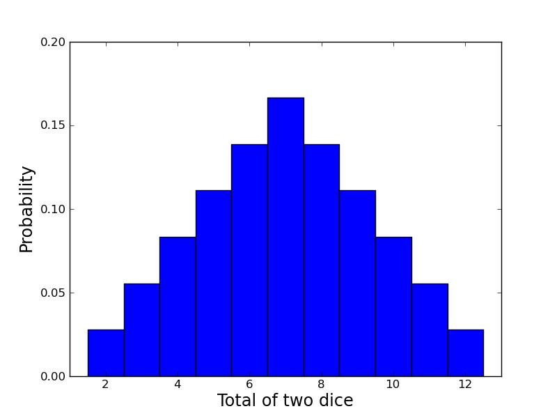
7

8 The need for sampling More commonly, we don't know the precise shape of the population's distribution on some variable. But we'd like to know. We have no alternative but to sample the population in some way. This might mean empirical sampling: we go out into the middle of the Pacific and catch 100 fish in order to learn something about the distribution of fish weights. It might mean sampling from many repeated runs of a simulation.

9 Samples A sample is just a group of observations drawn in some way from a wider population. Statistics has its roots in the effort to figure out just what you can reasonably infer about this wider population from the sample you've got. The size of your sample turns out to be an important limiting factor.

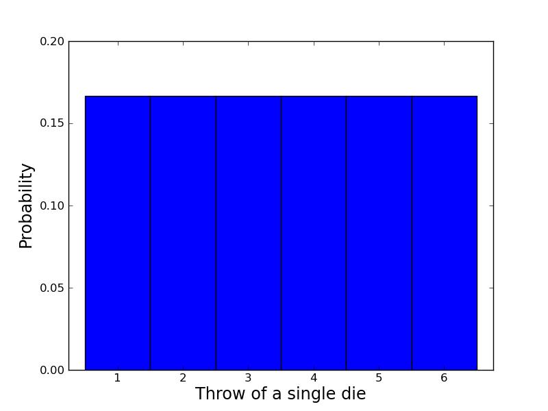
10 Sampling from a known distribution How can we learn about the effects of sampling? Let's take a very simple distribution that we understand well: the results from throwing a single die (i.e., the uniform distribution across the integers from 1 to 6 inclusive). We know that the mean of this distribution is 3.500, the variance is 2.917, and the standard deviation is Mean = ( ) / 6 = 3.5. Variance = ( (1-3.5)^2 + (2-3.5)^ (6-3.5)^2 ) / 6 =

11 Sampling from a known distribution Standard deviation = sqrt(variance) = We can simulate drawing some samples from this distribution to see how the size of our sample affects our attempts to draw conclusions about the population. What would samples of size one look like? That would just mean drawing a single variate from the population, i.e., throwing a single die, once.

12

13 Some samples A small sample of 3 observations gives a mean of A larger sample of 25 observations gives a mean of

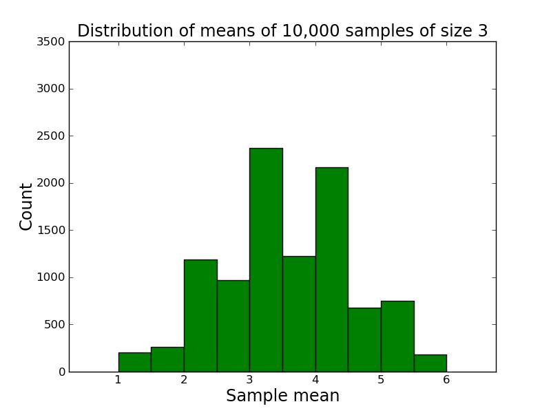
14 Samples give us varying results In both cases we didn't reproduce the shape of the true distribution nor get exactly 3.5 as the mean, of course. The bigger sample gave us a more accurate estimate of the population mean which is hopefully not too surprising. But how much variation from the true mean should we expect if we kept drawing samples of a given size? This leads us to the "meta-property" of the sampling distribution of the mean: let's simulate drawing a size 3 sample 10,000 times, calculate the sample mean, and see what that distribution looks like...

15

16 Sample distribution of the mean For the sample-size-3 case, it looks like the mean of the sample means centres in on the true mean of 3.5. But there's a lot of variation. With such a small sample size, we can get extreme results such as a sample mean of 1 or 6 reasonably often. Do things improve if we look at the distribution of the sample means of sample of size 25 for example?

17

18

19 Sample distribution of the mean So there are a few things going on here... The distribution of the sample means looks like it is shaped like a bell curve, despite the fact that we've been sampling from a flat (uniform) distribution. The width of the bell curve is getting gradually smaller as the size of our samples go up. So bigger samples seem to give tighter, more accurate estimates. Even for really small sample sizes, like 3, the sample mean distribution looks like it is centred on the true mean, but for a particular sample we could be way off.

20 Sample distribution of the mean Given our usual tools of means, variances, standard deviations, etc., we might ask how to characterize these sample distributions? It looks like the mean of the sample means will be the true mean, but what will happen to the variance / standard deviation of the sample means? Can we predict, for example, what the variance of the sample mean distribution would be if we took an infinite number of samples of a given size N?

21 Distribution arithmetic revisited We talked last week about taking the distribution of die-a throws and adding it to the distribution of die-b throws to find out something about two-dice throws. When two distributions are "added together", we know some things about the resulting distribution: The means are additive. The variances are additive. The standard deviations are not additive.

22 Distribution arithmetic revisited A question: what about dividing and multiplying distributions by constants? How does that work?

23 Distributional arithmetic revisited Scaling a distribution (multiplying or dividing by some constant) can be thought of as just changing the labels on the axes of the histogram. The mean scales directly. E[cX ]=c E[ X ] This time it's the variance that does not scale directly. V [cx ]=E[(cX) 2 ] E[cX ] 2 =c 2 V [ X ] The standard deviation (in the same units as the mean) scales directly. SD[cX ]= V [cx ]=c SD [X ]

24 Distributional arithmetic revisited When we calculate the mean of a sample, what are we really doing? For each observation in the sample, we're drawing a score from the true distribution. Then we add those scores together. So the mean and variance will be additive. Then we divide by the size of the sample. So the mean and standard deviation will scale by 1/N.

25 Some results For the 1-die case: Mean of the sample total will be 3.5 x N. Variance of the sample total will be x N. Standard deviation of the total will be sqrt(2.917n). Then we divide through by N... The mean of the sample means will be 3.5 (easy). The variance of the sample means will be / N (tricky: have to calculate the SD first). The standard deviation of the sample means will be sqrt(2.917n) / N (easy) which comes out as / sqrt(n).

26 What do we have now? We know that if we repeatedly sample from a population, taking samples of a given size N: The mean of our sample means will converge on the true mean: great news! The standard deviation of our distribution of sample means will tighten up in proportion to 1 / sqrt(n). In other words, accuracy improves with bigger sample sizes, but with diminishing returns. Remember this 1 / sqrt(n) ratio; it's related to something called the standard error which we'll come back to.

27 What do we have now? We also have a strong hint that the distribution of our sample means will itself take on a normal or bell curve shape, especially as we increase the sample size. This is interesting because of course the population distribution in this case was uniform: the results from throwing a single die many times do not look anything like a bell curve.

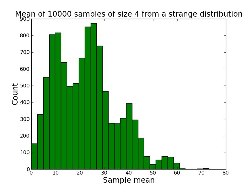
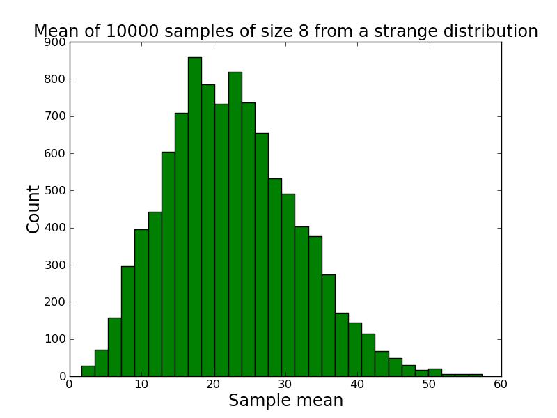
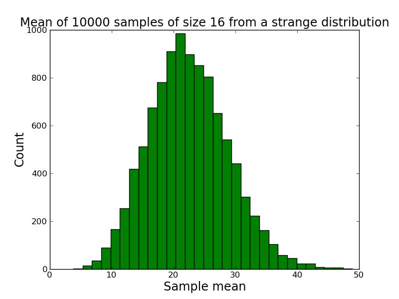
28 An unusual distribution How strong is this tendency for the sample means to be themselves normally distributed? Let's take a deliberately weird distribution that is as far from normal as possible and simulate sampling from it...

29

30 Central limit theorem The central limit theorem states that the mean of a sufficiently large number of independent random variables will itself be approximately normally distributed. Let's look at the distribution of the sample means for our strange distribution, given increasing sample sizes. At first glance, given its tri-modal nature, it's not obvious how we're going to get a normal (bell-shaped) distribution out of this.

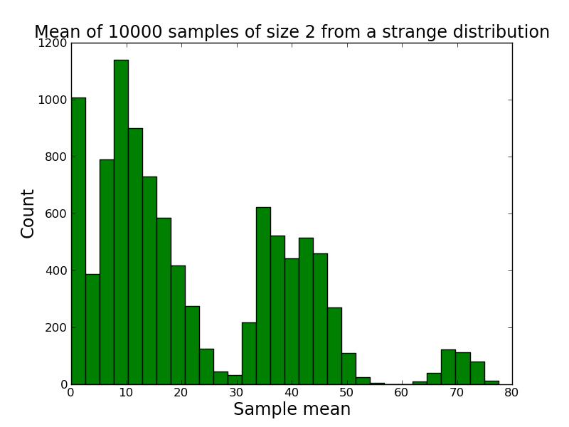
31

32

33

34

35

36

37

38 Central limit theorem We do reliably get a normal distribution when we look at the distribution of sample means, no matter how strange the original distribution that we were sampling from. This surprising result turns out to be very useful in allowing us to make inferences about populations from samples. Python code for the graphs and distributions in this lecture.

39 Central limit theorem more formally Consider a set of identically distributed random variables X i with zero mean and variance 2. Then we have: Where: X X n n is the normal distribution. N (0,σ 2 ) N (μ,σ 2 )= π σ exp( (x μ) ) 2 2σ 2 Remarks: Can always subtract mean... so this is general enough Convergence is in distribution, i.e. not uniform in centre and tails! (Chernoff's bound, Berry-Esseen theorem) Finite variance required here... other versions available

40 Central limit theorem more formally Consider a set of identically distributed random variables X i with zero mean and variance 2. Then we have: Where: X X n n is the normal distribution. N (0,σ 2 ) N (μ,σ 2 )= π σ exp( (x μ) ) 2 2σ 2 Remarks: Can always subtract mean... so this is general enough Convergence is in distribution, i.e. not uniform in centre and tails! Finite variance required here... other versions available

41 Central limit theorem Why? The normal distribution has some special properties, e.g.: X 1 N (μ 1, σ 1 2 ), X 2 N (μ 2, σ 2 2 ) X 1 + X 2 N (μ 1 +μ 2, σ 1 2 +σ 2 2 ) X N (μ, σ 2 ) cx N (cμ, c 2 σ 2 ) One can even recover the normal distribution from these properties, i.e. N (0,1)+N (0,1)= 2 N (0,1) defines the normal distribution (up to scaling). Now, in the CLT, consider convergence to some hypothetical distribution D X X n n D X X n + X n X 2n 2 n D Hence we expect D+ D= 2 D the limiting distribution to be normal

42 Central limit theorem Why? So... it is easy to see that convergence would happen to a normal distribution What is not quite so easy to see is that convergence takes place at all. The proof is best done via generating functions, but we won't do it here. Useful to know there are generalised versions of the CLT for cases when: The Xi's are not identically distributed The variance is infinite