Fluid Mechanics (3) - MEP 303A For THRID YEAR MECHANICS (POWER)
|
|
|
- Myra White
- 5 years ago
- Views:
Transcription

 Part (3)")

1 كلية الھندسة- جامعة القاھرة قسم ھندسة القوى الميكانيكية معمل التحكم األوتوماتيكى Notes on the course Fluid Mechanics (3) - MEP 303A For THRID YEAR MECHANICS (POWER) Part (3) Frictionless Incompressible Flow Compiled and Edited by Dr. Mohsen Soliman 2017/2018
2 Table of Contents of Part (3) Sec. Page 3.1 Introduction and Review Conservation of Mass Stream Function The Geometric Meaning of ψ Stream Function for Steady Plane Compressible Flow Stream Function for Incompressible Plane Flow in Polar Coordinates Stream Function for Incompressible Axisymmetric Flow Graphical Superposition of Stream Function of Plane Flows Vorticity and Irrotationality Conservation of Linear Momentum (Navier-Stokes Equations) Irrotational Flow Fields Case of Frictionless and Irrotational Flow (Euler s Equations) The Velocity Potential, Φ The Orthogonality of Stream Lines and Potential Lines The Generation of Rotationality Some Illustrative Plane Potential Flows Uniform Flow Source and Sink Vortex Doublet Superposition of Basic, Plane Potential Flows Source in a Uniform Stream Half-Body A sink plus a Vortex at the Origin Flow Past a Vortex An Infinite Row of Vortices The Vortex Sheet Rankine Ovals Flow Around a Circular Cylinder Flow Around a Cylinder with Circulation The Kelvin Oval Potential Flow Analogs Other Plane Potential Flows [The Complex Potential W(z)] 49 Summary of Complex Potentials for Elementary Plane Flows Uniform Stream at an Angle of Attack Line Source at Point Zo Line Vortex at Point Zo 50 Dr. Mohsen Soliman -2-
3 Sec. Page Flow around a Corner of Arbitrary Angle Flow Normal to a Flat Plate Complex Potential of The Dipole Flow Complex Potential of a Doublet Complex Potential of Flow around A Cylinder Flow Around A Cylinder With Nonzero Circulation The Method of Images Axisymmetric Potential Flows Spherical Polar Coordinates Uniform Stream in the x-direction Point Source or Sink Point Doublet Uniform Stream Plus a Point Source Uniform Stream Plus a point Doublet (Flow Around a Sphere) The Concept of Hydrodynamic Mass Other Aspects of Potential Flow Analysis Additional Advanced Potential Flows Other Aspects of Differential Analysis Numerical Methods The Finite Difference Method The Finite Element Method Case Study: Numerical Solution of Flow Around a Cylinder The Streamlines The Streaklines The Velocity Field The Pressure Field Forces Acting On The Cylinder Flow Around An Airfoil The Streamlines The Streaklines The Velocity Field The Pressure Field Forces On Airfoil Trailing and Railing Vortices 78 Questions for the Oral Exam, Frictionless Flow ( Part 3) 82 References 85 Problems 85 Dr. Mohsen Soliman -3-
* Frictionless Incompressible Flow The effect of viscosity can be neglected in many parts of most real viscous flow fields especially for external flow fields.")

4 Why Do we Study Frictionless Flow?: Part (3)* Frictionless Incompressible Flow The effect of viscosity can be neglected in many parts of most real viscous flow fields especially for external flow fields. It was found that viscous effects are important only near any solid boundaries in a small thin layer called the boundary layer. 3.1 Introduction and Review: Ref.:(1) Bruce R. Munson, Donald F. Young, Theodore H. Okiishi Fundamental of Fluid Mechanics 4 th ed., John Wiley & Sons, Inc., (2) Frank M. White Fluid Mechanics, 4 th ed. McGraw Hill, Dr. Mohsen Soliman -4-
5 3.1.1 Conservation of Mass: From Part (1) we found the differential form of the mass conservation equation: Dr. Mohsen Soliman -5-
6 3.1.2 Stream Function: Also from Part (1) we defined the stream function, ψ, for 2-D flow only as: If we recall that the linear momentum equation is: Dr. Mohsen Soliman -6-
7 3.1.3 The Geometric Meaning of ψ : Dr. Mohsen Soliman -7-


8 Example 3.1: Dr. Mohsen Soliman -8-
9 Example 3.2: Dr. Mohsen Soliman -9-

10 3.1.4 Stream function for Steady Plane Compressible Flow: Dr. Mohsen Soliman -10-

11 3.1.5 Stream function for Incompressible Plane Flow in Polar Coordinates: Stream function for Incompressible Axisymmetric Flow: Dr. Mohsen Soliman -11-
12 Example 3.3: Dr. Mohsen Soliman -12-
13 3.1.7 Graphical Superposition of Stream Functions of Plane Flows: Vorticity and Irrotationality: Dr. Mohsen Soliman -13-
14 3.2 Conservation of Linear Momentum (Navier-Stokes Equations): Also from Part (1) we defined the Conservation of Linear Momentum as: Dr. Mohsen Soliman -14-

15 Dr. Mohsen Soliman -15-
16 3.2.1 Irrotational Flow Fields: Dr. Mohsen Soliman -16-


17 Dr. Mohsen Soliman -17-
18 3.2.2 Case of Frictionless and Irrotational Flow (Euler s Equations): Dr. Mohsen Soliman -18-
19 3.2.3 The Velocity Potential, Φ : The Orthogonality of Stream Lines and Potential Lines: Dr. Mohsen Soliman -19-
20 3.2.5 The Generation of Rotationality: Dr. Mohsen Soliman -20-
21 Example 3.4: Dr. Mohsen Soliman -21-

22 Example 3.5: Dr. Mohsen Soliman -22-
23 3.3 Some Illustrative Plane Potential Flows: Dr. Mohsen Soliman -23-
24 Dr. Mohsen Soliman -24-
25 3.3.1 Uniform Flow: Source and Sink: Dr. Mohsen Soliman -25-
26 Example 3.6: Vortex: Dr. Mohsen Soliman -26-
27 Dr. Mohsen Soliman -27-
28 Circulation: Dr. Mohsen Soliman -28-


29 Example 3.7: Solution: Doublet: Dr. Mohsen Soliman -29-
30 Dr. Mohsen Soliman -30-

31 Dr. Mohsen Soliman -31-
32 Dr. Mohsen Soliman -32-

33 Example 3.8: Dr. Mohsen Soliman -33-


34 Some Notes on the case of Rankine Half-body: Boundary Layer Separation on Rankine half-body: Dr. Mohsen Soliman -34-

35 Example 3.9: Example 3.10: Dr. Mohsen Soliman -35-
36 3.4.2 A sink plus a Vortex at the Origin: Flow Past a Vortex: Dr. Mohsen Soliman -36-

37 3.4.4 An Infinite Row of Vortices: Dr. Mohsen Soliman -37-

38 3.4.5 The Vortex Sheet: 3.5 Rankine Ovals: Dr. Mohsen Soliman -38-
39 Dr. Mohsen Soliman -39-
40 Dr. Mohsen Soliman -40-
41 Dr. Mohsen Soliman -41-


42 Example 3.11: Dr. Mohsen Soliman -42-
43 3.7 Flow Around a Cylinder with Circulation: Dr. Mohsen Soliman -43-

44 Dr. Mohsen Soliman -44-

45 The Kutta-Joukowiski Lift Theorem: Experimental Lift and Drag of Rotating Cylinder: Dr. Mohsen Soliman -45-


46 Example 3.12: E3.12 Dr. Mohsen Soliman -46-


47 3.8 The Kelvin Oval: 3.9 Potential Flow Analogs: Dr. Mohsen Soliman -47-


48 Example 3.13: Dr. Mohsen Soliman -48-
49 3.10 Other Plane Potential Flows [The Complex Potential W(z)]: Dr. Mohsen Soliman -49-
50 Summary of Complex Potentials for Elementary Plane Flows: Uniform Stream at an Angle of Attack: Line Source at Point Zo: Line Vortex at Point Zo: Flow around a Corner of Arbitrary Angle : Dr. Mohsen Soliman -50-
51 Fig Streamlines for Corner angle β of a) 60 o, b) 90 o, c) 120 o, d) 270 o, and e) 360 o Flow Normal to a Flat Plate: Dr. Mohsen Soliman -51-
52 Fig.3.32 Streamlines in upper half-plane for flow normal to a flat plate of height 2a: a) continuous potential-flow theory; b) actual measured flow pattern; c) discontinuous potential theory with k 1.5 Dr. Mohsen Soliman -52-

 and (a,0) respectively).")
53 Complex Potential of The Dipole Flow: We now analyze the case of the so-called hydrodynamic dipole, which results from the superposition of a source and a sink of equal intensity placed symmetrically with respect to the origin. The analogy with electromagnetism is evident. The magnetic field induced by a wire in which a current flows satisfies equations that are similar to those governing irrotational plane flows. The complex potential of a dipole is (if the source and the sink are positioned in (-a,0) and (a,0) respectively). Streamlines are circles, the center of which lie on the y- axis and they converge obviously at the source and at the sink. Equipotential lines are circles, the center of which lie on the x-axis Complex Potential of a Doublet: A particular case of dipole is the so-called doublet, in which the quantity a tends to zero so that the source and sink both move towards the origin. The complex potential of a doublet is obtained making the limit of the dipole potential for vanishing a with the constraint that the intensity of the source and the sink must correspondingly tend to infinity as a approaches zero, the quantity Being constant (if we just superimpose a source and sink at the origin the resulting potential would be W=0) Dr. Mohsen Soliman -53-


54 Hint: develop ln (z+a) and ln(z-a) in a Taylor series in the neighborhood of the origin, assuming small a Complex Potential of Flow around A Cylinder: The superposition of a doublet and a uniform flow gives the complex potential That is represented here in terms of streamlines and equipotential lines. Note that one of the streamlines is closed and surrounds the origin at a constant distance equal to Recalling the fact that, by definition, a streamline cannot be crossed by the fluid, this complex potential represents the irrotational flow around a cylinder of radius R approached by a uniform flow with velocity U. Moving away from the body, the effect of the doublet decreases so that far from the cylinder we find, as expected, the undisturbed uniform flow. In the two intersections of the x-axis with the cylinder, the velocity is found to be zero. These two points are thus called stagnation points FLOW AROUND A CYLINDER WITH NONZERO CIRCULATION: In the last example, we superimpose to the complex potential that gives the flow around a cylinder a vortex of intensity positioned at the center of the cylinder. The resulting potential is The presence of the vortex does not alter the streamline describing the cylinder, while the two stagnation points below the x- axis. The streamlines are closer to each other on the upper part of the cylinder and more distant on the lower part. This indicates that the flow is accelerated on the upper face of the cylinder and decelerated on the lower part, with respect to the zero circulation case. The resulting flow field corresponds to the case of a rotating cylinder, which accelerates (with respect to the case of no circulation) fluid particles on part of the cylinder and decelerates them on the remainder of the cylinder. Note the presence of a discontinuity in the potential function (thick yellow line on the left) that is related to the fact that the vortex potential (as mentioned in a previous section) has a nonzero cyclic constant. Dr. Mohsen Soliman -54-


55 3.11 The Method of Images: Dr. Mohsen Soliman -55-

56 Example 3.14: Dr. Mohsen Soliman -56-
57 3.12 Axisymmetric Potential Flows: Spherical Polar Coordinates: Dr. Mohsen Soliman -57-
58 Uniform Stream in the x-direction: Point Source or Sink: Point Doublet: Dr. Mohsen Soliman -58-

:")
59 Uniform Stream Plus a Point Source: Uniform Stream Plus a point Doublet (Flow Around a Sphere): Dr. Mohsen Soliman -59-


60 3.13 The Concept of Hydrodynamic Mass: Dr. Mohsen Soliman -60-

61 Dr. Mohsen Soliman -61-

62 3.15 Additional Advanced Potential Flows Up to this point, we do not have any particular convenience in representing the flow in the complex plane. The full potential of this choice will become clear as soon as we introduce conformal mapping techniques. Let the following function Be an analytic function. It follows that also the inverse function z (z') is analytic. Consider the two planes z and The above function creates a link between a point in the z plane and a point in the z' plane. We can state that it maps one plane to the other. This transformation is said to be conformal because it does not affect angles, in the sense that given two lines in the z plane that intersect with some angle, the two transformed lines in the z' plane intersect with the same angle. In particular, two orthogonal families of curves in the z plane map into two other orthogonal families of curves in the z' plane. It follows that a conformal transformation maps equipotential and stream lines of an irrotational flow in the z plane into the corresponding lines of another irrotational flow in the z' plane. Given a flow field in the z plane with complex potentialw (z), the function: Is analytic because both W (z) and z (z') are analytic. In other words, the derivative Dr. Mohsen Soliman -62-

63 Exists and is unique because the derivatives on the right hand side exist and are unique. Therefore, W' is the complex potential of an irrotational inviscid flow in the z' plane. If P and P' are two corresponding points in the z and z' planes, respectively, And So that the two complex potentials W and W' assume the same value in corresponding points of the two domains.circulation along any (corresponding) closed line has also the same value in the two spaces because it is given by the integrals That are equal because along the two lines C and C', the potentials assume the same value.among the conformal transformations, the Joukowski transformation is relevant for the study of flow around a wing, because it maps the domain around a cylinder into the domain around a wing, whose thickness and curvature can be varied. The Joukowski Transformation: We introduce the conformal transformation due to Joukowski (who is pictured above) And analyze how a cylinder of radius R defined in the z plane maps into the z' plane: 1. If the circle is centered at (0, 0) and λ = R the circle maps into the segment between -2λ and +2λ lying on the x-axis; 2. If the circle is centered at (x c,0) and λ = R - x c, the circle maps in an airfoil that is symmetric with respect to the x'-axis; 3. If the circle is centered at (0, y c ) and λ = (R 2 y 2 c), the circle maps into a curved segment; 4. If the circle is centered at (x c, y c ) and λ = - x c + (R 2 y 2 c),, the circle maps into an asymmetric airfoil. To summarize, moving the center of the circle along the x-axis gives thickness to the airfoil, moving the center of the circle along the y-axis gives camber to the airfoil. In the following interactive application it is possible to move the center of the circle in the z plane and see the resulting transformed airfoil. The site is (http: ) We need to introduce some notations on airfoils. Dr. Mohsen Soliman -63-


64 The generic Joukowski airfoil has a rounded leading edge and a cusp at the trailing edge where the camber line forms an angle 2 β with the chord line. In the cylinder plane, β is related to the vertical coordinate of the center of the cylinder so that Usually the angle of attack (sometimes called physical) is defined as the angle that the uniform flow forms with the chord line. More interesting for aerodynamics is the angle In fact, when the angle is zero, the lift, as will be shown, vanishes. Then the angle is often defined as the effective angle of attack. Dr. Mohsen Soliman -64-


65 Numerical Methods: Dr. Mohsen Soliman -65-

66 Example 3.15: on Numerical Methods: Dr. Mohsen Soliman -66-
67 Dr. Mohsen Soliman -67-
68 The Finite Difference Method: Dr. Mohsen Soliman -68-
:")
69 Example 3.16 (Also on Numerical Methods): Dr. Mohsen Soliman -69-


70 Dr. Mohsen Soliman -70-


71 Dr. Mohsen Soliman -71-

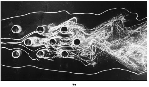
 separation of the boundary layer with the formation of a wake will be unavoidable for the cylinder.")
72 The Finite Element Method: 3.17 Case Study: Numerical Solution of Flow Around a Cylinder: In this section, we will analyze in more detail the irrotational flow field around a cylinder due to a uniform flow. The cylinder is a bluff body whereas a wing that is well-oriented (small angle of attack) with respect to flow is a slender body. In reality (in the sense of a real viscous fluid) separation of the boundary layer with the formation of a wake will be unavoidable for the cylinder. The irrotational solution cannot predict such phenomenon and the resulting flow field do not resemble the real flow around a cylinder. Given these, why do we study the irrotational flow around a cylinder? First of all, this flow is a good example of an irrotational flow in a relatively complex geometry. Secondly, and most important, because using conformal mapping we can transform the flow around a cylinder into the flow around a Joukowski wing. If a wing profile is well oriented with respect to the uniform flow, boundary layer separation is negligible and the pressure field obtained by means of the irrotational flow solution can be considered as a good approximation of the actual pressure field. Therefore, the resulting lift is in good agreement with experimental measurements. In the following sections several animations show how the velocity and pressure fields vary as the circulation around the cylinder is changed THE STREAMLINES: The first animation is for the velocity field, represented here in term of the stream function. For a case of zero circulation, the velocity field is symmetric with respect to the x-axis and the two stagnation points lie at the intersections of the cylinder and the x-axis (left figure). The animation on the right shows the stream function as the circulation increases to a maximum and then decreases to zero. The uniform flow is from right to left and the circulation is counterclockwise. You can see the stagnation points moving towards the lower face of the cylinder as circulation increases. The streamlines become closely packed near the upper face and less packed near the lower face, indicating an acceleration on the upper face and a deceleration on the lower face. In fact, the mass flux in the stream tube defined by two adjacent streamlines is constant. When streamlines get closer to each other, the flow is accelerating and vice versa. Dr. Mohsen Soliman -72-


73 THE STREAKLINES: The streaklines displayed in the following animations are the result of an ideal experiment in which a passive tracer (like smoke) is injected in the flow, making the path of ``marked'' fluid particles visible. This allows us to follow, in a Lagrangian sense, the motion of the group of fluid particles that have passed through the same point. Since the flow is steady, the trajectories of such particles (the streaklines) are identical to the streamlines. Changing periodically the color of all the smoke sources allows for a visualization of the time history of subsets of smoke particles injected in the same time interval. When the colored lines become shorter, the marked fluid particles are slowing down and vice versa. The grid of smoke sources is equally spaced in the vertical direction and it is positioned far upstream from the body (at a distance of about 100 times the radius of the cylinder), so that sources are not influenced by the body (uniform flow). Animations have been realized for three increasing values of the circulation around the cylinder. In the first animation, the circulation is zero and the flow is symmetrical with respect to the x-axis. Note how the fluid particles closer to the cylinder are delayed with respect to those passing well above (or below) the cylinder. This delay is not due to friction (we are dealing with an inviscid fluid) but to the fact that near the stagnation points velocity tends to decelerate to zero speed. Due to the symmetry of the flow field, if two particles start symmetrically with respect to the x-axis, they will need the same amount of time to flow around the body. When circulation is increased, the latter statement is not true anymore. Now, the fluid flowing above the cylinder reaches the downstream section before the fluid flowing below the cylinder. It is possible to demonstrate that the arrival times are the same only for two particles starting slightly above and below the front stagnation point and flowing along the cylinder surface. Dr. Mohsen Soliman -73-

74 In many elementary aerodynamics textbooks it is stated that, with non-zero circulation, the portion of fluid flowing above the cylinder is accelerated with respect to the one flowing below it ``because it must travel for a longer route to reach downstream in the same amount of time''. In reality there is no physical law imposing that the two fluid portions flowing above and below the cylinder (the interface of which can be identified with the streamline passing through the two stagnation points) must take the same time to travel around the cylinder. Indeed, looking at the second animation, it is evident that far from the body, where the flow is essentially uniform, the ``above-the cylinder'' fluid reaches the left end of the window well before the ``below-the cylinder'' fluid does. If we were allowed to observe what happens far downstream, where the flow is certainly uniform again, we would see that this configuration is somewhat ``frozen'' and the fluid particles which have been delayed do not try in any way to catch up. In the cases examined so far, it is nevertheless still true that two adjacent fluid particles that are separated by the body will become adjacent again once the body is passed, since the arrival times of two particles flowing along the cylinder surface are the same. In the case of flow around an airfoil even the latter statement is true only for a very peculiar case THE VELOCITY FIELD: The animation of the velocity vector field confirms what has been shown in the stream function animation. When circulation is zero, the uniform stream approaching from the right divides into two symmetric flows, one going over the cylinder, the other flowing under it. The two flows connect again downstream of the cylinder. The flow field is symmetric with respect to the x-axis. Two fluid particles immediately above and below the upstream stagnation point travel the same distance around the cylinder and then meet again at the downstream stagnation point. When circulation is increased, the stagnation points move towards the lower half of the cylinder so that the two companion fluid particles follow different routes to reach the downstream stagnation point. In particular the fluid particle that travels above the cylinder makes a longer route with respect to its companion, but it travels fast enough to arrive at the same time at the downstream stagnation point THE PRESSURE FIELD: We can now evaluate the pressure field with the equivalence: Dr. Mohsen Soliman -74-

. As circulation increases the pressure field is still symmetric with respect to the y-axis but becomes asymmetric with respect to the x-axis. 3.17.")
75 Where indicates the reference value of the pressure at infinity (where the flow is uniform). In the picture, shown is the excess nondimensional pressure defined as : When circulation is absent, the pressure field is symmetric with respect to both the x and the y- axes. On the stagnation points the excess pressure is positive (which means an action directed towards the body) while on the upper and lower points the excess pressure is negative (which means an action directed away from the body). As circulation increases the pressure field is still symmetric with respect to the y-axis but becomes asymmetric with respect to the x-axis FORCES ACTING ON THE CYLINDER: To understand the implication of the asymmetry of the pressure field in terms of the forces acting on the cylinder, the last animation shows the elementary forces as vectors on the cylinder surface. Each elementary force is given by Where p is pressure, is the normal unit vector directed away from the surface and ds is the surface arc. The resulting force (the vectorial sum of all the elementary forces on the body) is clearly zero when circulation is zero (D'Alambert paradox). As circulation increases the component of the resulting force in the direction of the uniform flow is still zero (no drag), whereas a component in the direction perpendicular to the uniform flow (lift) appears that increases as circulation is enhanced. The modulus of the lift can be evaluated analytically (Kutta- Joukowski theorem) and is 3.18 FLOW AROUND AN AIRFOIL: Before analyzing the velocity and pressure field for the case of an airfoil, we need to investigate a little more deeply the role played by circulation. The Kutta-Joukowski theorem shows that lift is proportional to circulation, but apparently the value of the circulation can be assigned arbitrarily. The solution of flow around a cylinder tells us that we should expect to find two stagnation points along the airfoil the position of which is determined by the circulation around the profile. There is a particular value of the circulation that moves the rear stagnation point (V=0) exactly on the trailing edge. This condition, which fixes a value of the circulation by simple geometrical considerations is the Kutta condition. Using Kutta condition the circulation is not anymore a free variable and it is possible to evaluate the lift of an airfoil using the same techniques that were described for the cylinder. Note that the flow fields obtained for a fixed value of the circulation are all valid solutions Dr. Mohsen Soliman -75-
76 of the flow around an airfoil. The Kutta condition chooses one of these fields, one that represents the best actual flow. We can try to give a feasible physical justification of the Kutta condition; to do this we need to introduce a concept that is ignored by the theory for irrotational inviscid flow: the role-played by the viscosity of a real fluid. Suppose we start from a static situation and give a small velocity to the fluid. If the fluid is initially at rest it is also irrotational and, neglecting the effect of viscosity, it must remain irrotational due to Thompson theorem. The flow field around the wing will then have zero circulation, with two stagnation points located one on the lower face of the wing, close to the leading edge, and one on the upper face, close to the trailing edge. A very unlikely situation is created at the trailing edge: a fluid particle on the lower side of the airfoil should travel along the profile, make a sharp U-turn at the trailing edge, go upstream on the upper face until it reaches the stagnation point and then, eventually, leave the profile. A real fluid cannot behave in this way. Viscosity acts to damp the sharp velocity gradient along the profile causing a separation of the boundary layer and a wake is created with shedding of clockwise vorticity from the trailing edge. Since the circulation along a curve that includes both the vortex and the airfoil must still be zero, this leads to a counterclockwise circulation around the profile. But if a nonzero circulation is present around the profile, the stagnation points would move and in particular the rear stagnation point would move towards the trailing edge. The sequence vortex shedding -> increase of circulation around the airfoil -> downstream migration of the rear stagnation point continues until the stagnation point reaches the trailing edge. When this happens the sharp velocity gradient disappears and the vorticity shedding stops. This ``equilibrium'' situation freezes the value of the circulation around the airfoil, which would not change anymore. Let us now proceed to examine the velocity and pressure fields around an airfoil with the aid of some animations showing how they vary when the (effective) angle of attack is changed. In each shot the flow field is obtained imposing the Kutta condition to determine the circulation. A sequential browsing of the following pages is suggested, at least for first time visitors THE STREAMLINES: In the following animation the stream function is plotted together with the streamlines. Direction of flow is from right to left and the angle of attack is varied by rotating the airfoil. Note that, as the airfoil rotates, a streamline always leaves the trailing edge, indicating that Kutta condition is imposed. Far from the airfoil the streamlines tend to become horizontal, as expected for a uniform flow. Dr. Mohsen Soliman -76-

 have been chosen for the animations.")
77 THE STREAKLINES: In the following animations the streaklines generated by a set of smoke sources equally spaced in the vertical direction and positioned far upstream of the airfoil are presented. The color of the injected smoke has been changed at regular time steps so as to make the time history of the fluid particles that have been ``marked'' passing through each smoke source visible. Three increasing values of the effective angle of attack (0, 15 and 30 degrees, respectively) have been chosen for the animations. The first animation shows a smoke pattern similar to that observed for the flow around a cylinder with no circulation. Indeed, in this case the rear stagnation point is naturally coincident with the trailing edge and the Kutta condition is verified with zero circulation around the airfoil. Note how the fluid particles closer to the airfoil are delayed with respect to those passing well above (or below) the airfoil. Friction has no role here and this effect, as for the cylinder, is due to the vanishing of velocity in the neighborhood of the stagnation points. Also note how the two portions of fluid passing above and below the airfoil reach the left end section at the same time. Two fluid particles flowing along the profile need the same time to travel above or below the airfoil. As the angle of attack, and so the circulation around the airfoil, is increased, the latter statement is not true anymore, in the sense that fluid flowing above the airfoil reach the downstream section earlier than the fluid traveling below it. It can be demonstrated that in contrast to what happens for the cylinder, the traveling times are in this case different also for fluid particles flowing along the airfoil surface, as it is evident looking at the animations above and focusing on the neighborhood of the trailing edge. This effect is related to the role played by the conformal transformation, which alters both the length of the path and the velocity but not in a way to keep the traveling times of two particles flowing along the surface of the airfoil equal. The fluid portion flowing below the airfoil is delayed with respect to the portion flowing Dr. Mohsen Soliman -77-

 peak of the pressure appears on the upper face of the airfoil close to the leading edge.")
. 3.18.5 FORCES ON AIRFOIL: We now examine the forces acting on the airfoil in terms of elementary forces instead of pressure.")
78 above it, and the delay increases as the angle of attack (and so the circulation around the airfoil and, as we will see, the lift) increases. Stating that the fluid flowing above the airfoil is accelerated with respect to the fluid flowing below it ``because it must travel for a longer route in the same time'' is then definitely wrong THE VELOCITY FIELD: This animation shows again the flow field, now described in terms of the velocity vectors THE PRESSURE FIELD: The pressure field shows positive (reddish) values on the lower face of the wing and negative (yellow-green-blue) values on the upper face, thus leading to a lift. Note that for large values of the angle of attack a strong negative (blue) peak of the pressure appears on the upper face of the airfoil close to the leading edge. As this negative peak increases, the positive pressure gradient downstream of it increases, a condition that leads to boundary layer separation on the upper face and consequently to a sudden drop in the lift (stall) FORCES ON AIRFOIL: We now examine the forces acting on the airfoil in terms of elementary forces instead of pressure. While it is intuitive that as the angle of attack increases the lift increases, it is not easy to see that the drag is always zero for the airfoil as it was for the cylinder. This is because the unit vector normal to the airfoil is not simply radial as in the cylinder case Tailing and Railing Vortices: On a clear day, trailing vortices are often seen in the sky following the passage of an airplane. The vortices are formed because the wing develops lift. That is, the pressure on the top of the wing is lower than on the bottom, and near the tips of the wing this pressure difference causes the air to move around the edge from the bottom surface to the top. This results in a roll-up of the fluid, which then forms the trailing vortex. In the sky, the vortex becomes visible when the air has a high Dr. Mohsen Soliman -78-


79 humidity. The velocities inside the vortex can be very high, and the pressure is therefore quite low. Water vapor in the air condenses as water droplets, and the droplets mark the presence of the vortex. In the picture below of a crop-duster flying near the ground, the vortex is made visible by a red flare placed on the ground. The red smoke is wrapped up by the trailing vortex originating near the tip of the wing. Picture courtesy of DANTEC Measurement Technology. The strength of the vortex is related to the amount of lift generated by the wing, so they become particularly strong in high-lift conditions such as take-off and landing. They also increase in strength with the size of the airplane, since the lift is equal to the weight of the airplane. For a large transport airplane such as a 747, the vortices are strong enough to flip a small airplane if it gets too close. Trailing vortices are therefore the principal reason for the time delay enforced by the FAA between take-offs and landings at airports. Railing vortices and downwash phenomenon of an aircraft in flight are seen clearly in the figure below. In this situation, a Cessna Citation VI was flown immediately above the fog bank over Lake Tahoe at approximately 313 km/h or 170 knots (B. Budzowski, Director of Flight Operations, Cessna Aircraft Company, private communication, 1993). Aircraft altitude was about 122 m (400 ft) above the lake, and the weight was approximately 8400 kg. As the trailing vortices descended over the fog layer due to the downwash, the flow field in the wake was made visible by the distortion of the fog layer. The photo was taken by P. Bowen for the Cessna Aircraft Company from the tail gun- ner's position in a B-25 flying in formation slightly above and ahead of the Cessna. The aircraft is seen initiating a gentle climb after a level flight, leaving a portion of the fog layer yet unaffected. The wingspan measured 16.3 m and the wing area was 29 m^2. The Reynolds number based on the mean aerodynamic chord of 2.1 m was 1.1x10^7. The figure below is extract from the Gallery of Fluid Motion, Physics of Fluids A, Vol. 5, September Contribution by Hiroshi Higuchi (Syracuse University). Dr. Mohsen Soliman -79-


80 Photo courtesy of Cessna Aircraft Company. As seen above, fluid simulation from SAAB Aircraft shows phase lag between upper and lower air parcels after an airfoil has passed. Air travels much faster over the top of the airfoil, and then it never rejoins the air, which has traveled below. Note that the airfoil has deflected the air downwards. Another picture is seen above from the 1993 Aviation Week & Space Technology Photo Contest. This came second in the Military category, and it was taken by James E. Hobbs, from Lockheed Aircraft service Co., Ontario, California. The plane is ejecting flares during a test of an infrared missile warning and self-protection system installed on a C-130 Hercules. The trailing vortices formed in the wake are clearly visible. The size of these vortices is related to the lift produced by the wings, and the photograph suggests that the aircraft was climbing during this maneuver. Dr. Mohsen Soliman -80-


81 This picture shows a SAAB JAS39 Gripen landing on a rainy roadbase. Downwash is made evident by the foggy cloud above the runaway. Some more downwash... this is a French Transall deploying flares. Dr. Mohsen Soliman -81-
82 Questions for the Oral Exam Frictionless Flow ( Part 3) 1- If the stream function, Ψ, is defined as Ψ=f(x,y) or Ψ=g(r,θ). What is the physical and mathematical meaning of these two functions. How can we get the stream function for a given flow field V(x,y). What is the relationship between the stream function, Ψ, and the vorticity vector (curl of V), linear momentum equations, and the Bernolli s equation in both real and ideal flows. Can we define Ψ=f(x,y,z) or Ψ=g(r,θ,z) for 3-D, steady, real viscous flow. Give some examples with sketches for Ψ If an Eulerian velocity flow field is defined as V= f(t,x,y,z), Explain the physical and mathematical meaning of this function. What do we mean by the total or substantial derivative? How do we get the acceleration, a, of this field? What is the deference between local acceleration and convective acceleration. In a steady flow, can the acceleration of the flow be non-zero? Explain your answer with an example Discuss what is wrong in the following statements (use sketches if needed): I. -The stream function, Ψ, represents the mass conservation eqn. 3-D viscous flow. II. -The value of Ψ function must be constant for all streamlines in 3-D viscous flow. III. -Values of Ψ function are the difference in the momentum flux between streamlines. IV. -The Laplace equation, 2 Ψ=0 represent the mass conservation equation for a 3-D frictionless flow field and can be solved to get pressure distribution in that flow field If the potential function, Φ, is defined as Φ =f(x,y) or Φ =g(r,θ). What is the physical and mathematical meaning of these two functions. How can we get the potential function for a given flow field V(x,y). What is the relationship between the potential function, Φ, and the vorticity vector (curl of V), linear momentum equations, and the Bernolli s equation in both real and ideal flows. Can we define Φ =f(x,y,z) or Φ =g(r,θ,z) for 3-D, steady, real viscous flow. Give some examples with sketches for Φ What do you know about Euler s equations?. Discuss how can these equation be reduced to Bernoulli s equation along streamline in frictionless flow?. In a frictionless flow field, can we apply Bernoulli s equation everywhere in the flow? How? Discuss what is wrong in the following statements (use sketches if needed):: I. In 3-D viscous flow, the stream function, Ψ, is parallel to the velocity potential function, Φ, and both of them can be used to get the pressure distribution in the flow. II. Euler s equations represent the mass conservation for 2-D laminar flow where the no slip condition (zero velocity at the wall) must be valid every where in the flow field. III. In a 3-D viscous flow, the complex potential function is defined as W(z) = (Ψ + i Φ) where z = (y + i x) and the velocity can be obtained from dw/dz= (v + i u) Discuss what is wrong in the following statements (use sketches if needed): I. In a 3-D viscous, rotational flow, the complex potential function for a uniform stream in the ve x-axis direction is defined as W(z) = U z e iα II. In a 3-D viscous, rotational flow, the complex potential function for a point source of strength, Q, located at point z o is defined as W(z) = -(Q/2Π) ln (z o - z). III. In a 3-D viscous, rotational flow, the complex potential function for a free, clockwise vortex located at point z o is defined as W(z) = - (iγ/2π) ln (z o - z). Dr. Mohsen Soliman -82-
83 8- In our study of Fluid Mechanics, we can use one of the following methods: a- Differential analysis method b- Integral analysis method c- Dimensional analysis method with some experimental work Explain very briefly those methods showing the main differences between them regarding the reason for, and the output result of each method. Give an example for each method. Do we neglect viscous effects in any of the above methods? Explain your answer In both real or ideal flow, define the physical meaning and the equation of (a) stream lines, (b) the no-slip condition. Give some examples in both internal flows and external flows. What is the difference between Ideal fluids or Newtonian fluids or Non-Newtonian fluids? Explain what do we mean by saying that the Eulerian Pressure scalar field is given as P = f(t,x,y,z) or P = g(t,r,θ,z)? What do we mean by the total or substantial derivative d/dt? How do we get dp/dt of the field P = f(t,x,y,z)? What is the deference between local pressure derivative and convective pressure derivative. In a steady flow, can the total or substantial pressure derivative of the flow be a non-zero value? Explain your answer with an example Prove that the time-derivative operator (called total or substantial derivative) following a fluid particle is: d/dt = / t + ( V. ), where is the gradient operator What do you know about the conservation equations in Fluid Mechanics? Using the differential analysis method, stat and discuss two of the main conservation equations of fluid mechanics. Show all the non-linear terms in those equations. What is the divergence of the velocity vector field?. Can we write the momentum equations for a Non-Newtonian fluid? How Using the cartesian coordinates, write down and discuss the meaning of each term and show all the differences you know between the Navier-Stoke s equations and the Euler s equations. Can we use Euler s equations to solve the flow in long pipes? Why? What is the relation between Euler s equations and Bernolli s equation? The flow rate is 0.25 m 3 /s into a convergent nozzle of 0.6 m height at entrance and 0.3m height at exit. Find the velocity, acceleration and pressure fields through the nozzle. (take the length of the nozzle=1.5m) The flow rate is 0.25 m 3 /s into a divergent nozzle of 0.3 m height at entrance and 0.6m height at exit. Find the velocity, acceleration and pressure fields through the nozzle. (take the length of the nozzle=1.5m) Which of the following motions are kinematically possible for incompressible flow (k and Q are constants): i) u = k x, v = k y, w = -2k z ii) V r = - Q/2Л r, V θ = k/2л r iii) V r = k cos θ, V θ = -k sin θ For a 2-D flow field in the xy-plane, the y component of the velocity is given by: v = y 2 2x + 2y. Determine a possible x-component for a steady incompressible flow. Is it also valid for unsteady flow? How many possible x-components are there? Why?. Dr. Mohsen Soliman -83-
84 18- For a 2-D flow field in the xy-plane, the x component of the velocity is given by: u = y 2 2x + 2y. Determine a possible y-component for a steady incompressible flow. Is it also valid for unsteady flow? How many possible x-components are there? Why? Prove that the equation of continuity for 2-D incompressible flow in polar coordinates is in the form: V r / r + V r /r + 1/r ( V θ / θ) = Explain the physical meaning and the mathematical equations for both the divergence operator and the curl operator as applied on a vector field. Take the velocity field V as an example. (hint: prove that the divergence of V = the rate of volume expansion of fluid element per unit initial volume). Prove also that for an incompressible velocity field, the divergence of V = 0. What is the relationship between the curle of V and the rotation in the velocity field Examine the following functions to determine if they could represent the velocity potential for an incompressible inviscid flow: a) Φ=2x+3y+4z 2 b) Φ = x + xy + xyz c) Φ = x 2 + y 2 + z The velocity potential of a steady field is given by the expression: Φ = 2xy + y, and the temperature is given by: T = x 2 + 3xy + 2. Find both the local and the convective parts of the rate of temperature change in this field Find the potential function, Φ, of a flow field such that the horizontal component of the velocity varies linearly along the y-axis and has the value U o on the x-axis. What is the stream function, Ψ, of this field Find the potential function, Φ, of a flow field such that the vertical component of the velocity varies linearly along the x-axis and has the value V o on the y-axis. What is the stream function, Ψ, of this field Velocity components of a 2-D flow are: u=k(y 2 -x 2 ) & v=2kxy, find the stream function which has Ψ=0 at the origin. Find the potential function Φ, sketch both the Ψ and Φ lines Velocity components of 2-D flow are: u=-a(y 2 -x 2 ) & v=-2axy, find the stream function which has Ψ=0 at the origin. Find the potential function Φ, sketch both the Ψ and Φ lines The velocity potential of a 2-D flow is: Φ=kxy, Find and sketch the stream lines Ψ. 28- The velocity potential of a 2-D flow is: Φ=y+x 2 -y 2, Find and sketch the stream lines Ψ Show that the 2-D flow: Ψ =x+2x 2-2y 2 is irrotational. What is the velocity potential Φ Find the exact equation for the stream lines Ψ of a flow of water around a 90 o solid corner if the velocity at the point (0,4) = +3 m/s. sketch both the Ψ and Φ lines. Dr. Mohsen Soliman -84-
85 Dr. Mohsen Soliman -85-

86 Dr. Mohsen Soliman

87 Dr. Mohsen Soliman -87-

88 Dr. Mohsen Soliman -88-
89 Dr. Mohsen Soliman -89-
90 Dr. Mohsen Soliman -90-
91 Dr. Mohsen Soliman -91-
PEMP ACD2505. M.S. Ramaiah School of Advanced Studies, Bengaluru
 Two-Dimensional Potential Flow Session delivered by: Prof. M. D. Deshpande 1 Session Objectives -- At the end of this session the delegate would have understood PEMP The potential theory and its application
Detailed Outline, M E 521: Foundations of Fluid Mechanics I
 Detailed Outline, M E 521: Foundations of Fluid Mechanics I I. Introduction and Review A. Notation 1. Vectors 2. Second-order tensors 3. Volume vs. velocity 4. Del operator B. Chapter 1: Review of Basic
V (r,t) = i ˆ u( x, y,z,t) + ˆ j v( x, y,z,t) + k ˆ w( x, y, z,t)
 = i ˆ u( x, y,z,t) + ˆ j v( x, y,z,t) + k ˆ w( x, y, z,t)") IV. DIFFERENTIAL RELATIONS FOR A FLUID PARTICLE This chapter presents the development and application of the basic differential equations of fluid motion. Simplifications in the general equations and common
IV. DIFFERENTIAL RELATIONS FOR A FLUID PARTICLE This chapter presents the development and application of the basic differential equations of fluid motion. Simplifications in the general equations and common
1. Introduction, tensors, kinematics
 1. Introduction, tensors, kinematics Content: Introduction to fluids, Cartesian tensors, vector algebra using tensor notation, operators in tensor form, Eulerian and Lagrangian description of scalar and
Chapter 6: Incompressible Inviscid Flow
 Chapter 6: Incompressible Inviscid Flow 6-1 Introduction 6-2 Nondimensionalization of the NSE 6-3 Creeping Flow 6-4 Inviscid Regions of Flow 6-5 Irrotational Flow Approximation 6-6 Elementary Planar Irrotational
1. Fluid Dynamics Around Airfoils
 1. Fluid Dynamics Around Airfoils Two-dimensional flow around a streamlined shape Foces on an airfoil Distribution of pressue coefficient over an airfoil The variation of the lift coefficient with the
Lifting Airfoils in Incompressible Irrotational Flow. AA210b Lecture 3 January 13, AA210b - Fundamentals of Compressible Flow II 1
 Lifting Airfoils in Incompressible Irrotational Flow AA21b Lecture 3 January 13, 28 AA21b - Fundamentals of Compressible Flow II 1 Governing Equations For an incompressible fluid, the continuity equation
SPC Aerodynamics Course Assignment Due Date Monday 28 May 2018 at 11:30
 SPC 307 - Aerodynamics Course Assignment Due Date Monday 28 May 2018 at 11:30 1. The maximum velocity at which an aircraft can cruise occurs when the thrust available with the engines operating with the
Fluid Dynamics: Theory, Computation, and Numerical Simulation Second Edition
 Fluid Dynamics: Theory, Computation, and Numerical Simulation Second Edition C. Pozrikidis m Springer Contents Preface v 1 Introduction to Kinematics 1 1.1 Fluids and solids 1 1.2 Fluid parcels and flow
Department of Mechanical Engineering
 Department of Mechanical Engineering AMEE401 / AUTO400 Aerodynamics Instructor: Marios M. Fyrillas Email: eng.fm@fit.ac.cy HOMEWORK ASSIGNMENT #2 QUESTION 1 Clearly there are two mechanisms responsible
Some Basic Plane Potential Flows
 Some Basic Plane Potential Flows Uniform Stream in the x Direction A uniform stream V = iu, as in the Fig. (Solid lines are streamlines and dashed lines are potential lines), possesses both a stream function
Detailed Outline, M E 320 Fluid Flow, Spring Semester 2015
 Detailed Outline, M E 320 Fluid Flow, Spring Semester 2015 I. Introduction (Chapters 1 and 2) A. What is Fluid Mechanics? 1. What is a fluid? 2. What is mechanics? B. Classification of Fluid Flows 1. Viscous
Fundamentals of Fluid Mechanics
 Sixth Edition Fundamentals of Fluid Mechanics International Student Version BRUCE R. MUNSON DONALD F. YOUNG Department of Aerospace Engineering and Engineering Mechanics THEODORE H. OKIISHI Department
High Speed Aerodynamics. Copyright 2009 Narayanan Komerath
 Welcome to High Speed Aerodynamics 1 Lift, drag and pitching moment? Linearized Potential Flow Transformations Compressible Boundary Layer WHAT IS HIGH SPEED AERODYNAMICS? Airfoil section? Thin airfoil
6.1 Momentum Equation for Frictionless Flow: Euler s Equation The equations of motion for frictionless flow, called Euler s
 Chapter 6 INCOMPRESSIBLE INVISCID FLOW All real fluids possess viscosity. However in many flow cases it is reasonable to neglect the effects of viscosity. It is useful to investigate the dynamics of an
Aerodynamics. Lecture 1: Introduction - Equations of Motion G. Dimitriadis
 Aerodynamics Lecture 1: Introduction - Equations of Motion G. Dimitriadis Definition Aerodynamics is the science that analyses the flow of air around solid bodies The basis of aerodynamics is fluid dynamics
Fundamentals of Fluid Dynamics: Ideal Flow Theory & Basic Aerodynamics
 Fundamentals of Fluid Dynamics: Ideal Flow Theory & Basic Aerodynamics Introductory Course on Multiphysics Modelling TOMASZ G. ZIELIŃSKI (after: D.J. ACHESON s Elementary Fluid Dynamics ) bluebox.ippt.pan.pl/
Inviscid & Incompressible flow
 < 3.1. Introduction and Road Map > Basic aspects of inviscid, incompressible flow Bernoulli s Equation Laplaces s Equation Some Elementary flows Some simple applications 1.Venturi 2. Low-speed wind tunnel
Given a stream function for a cylinder in a uniform flow with circulation: a) Sketch the flow pattern in terms of streamlines.
 Sketch the flow pattern in terms of streamlines.") Question Given a stream function for a cylinder in a uniform flow with circulation: R Γ r ψ = U r sinθ + ln r π R a) Sketch the flow pattern in terms of streamlines. b) Derive an expression for the angular
Question Given a stream function for a cylinder in a uniform flow with circulation: R Γ r ψ = U r sinθ + ln r π R a) Sketch the flow pattern in terms of streamlines. b) Derive an expression for the angular
FUNDAMENTALS OF AERODYNAMICS
 *A \ FUNDAMENTALS OF AERODYNAMICS Second Edition John D. Anderson, Jr. Professor of Aerospace Engineering University of Maryland H ' McGraw-Hill, Inc. New York St. Louis San Francisco Auckland Bogota Caracas
Department of Energy Sciences, LTH
 Department of Energy Sciences, LTH MMV11 Fluid Mechanics LABORATION 1 Flow Around Bodies OBJECTIVES (1) To understand how body shape and surface finish influence the flow-related forces () To understand
Fluid Mechanics Prof. T. I. Eldho Department of Civil Engineering Indian Institute of Technology, Bombay
 Fluid Mechanics Prof. T. I. Eldho Department of Civil Engineering Indian Institute of Technology, Bombay Lecture No. # 35 Boundary Layer Theory and Applications Welcome back to the video course on fluid
Chapter 3 Bernoulli Equation
 1 Bernoulli Equation 3.1 Flow Patterns: Streamlines, Pathlines, Streaklines 1) A streamline, is a line that is everywhere tangent to the velocity vector at a given instant. Examples of streamlines around
Mestrado Integrado em Engenharia Mecânica Aerodynamics 1 st Semester 2012/13
 Mestrado Integrado em Engenharia Mecânica Aerodynamics 1 st Semester 212/13 Exam 2ª época, 2 February 213 Name : Time : 8: Number: Duration : 3 hours 1 st Part : No textbooks/notes allowed 2 nd Part :
Syllabus for AE3610, Aerodynamics I
 Syllabus for AE3610, Aerodynamics I Current Catalog Data: AE 3610 Aerodynamics I Credit: 4 hours A study of incompressible aerodynamics of flight vehicles with emphasis on combined application of theory
Fundamentals of Aerodynamics
 Fundamentals of Aerodynamics Fourth Edition John D. Anderson, Jr. Curator of Aerodynamics National Air and Space Museum Smithsonian Institution and Professor Emeritus University of Maryland Me Graw Hill
INSTITUTE OF AERONAUTICAL ENGINEERING (Autonomous) Dundigal, Hyderabad
 Dundigal, Hyderabad") INSTITUTE OF AERONAUTICAL ENGINEERING (Autonomous) Dundigal, Hyderabad - 500 043 AERONAUTICAL ENGINEERING TUTORIAL QUESTION BANK Course Name : LOW SPEED AERODYNAMICS Course Code : AAE004 Regulation : IARE
INSTITUTE OF AERONAUTICAL ENGINEERING (Autonomous) Dundigal, Hyderabad - 500 043 AERONAUTICAL ENGINEERING TUTORIAL QUESTION BANK Course Name : LOW SPEED AERODYNAMICS Course Code : AAE004 Regulation : IARE
Continuum Mechanics Lecture 7 Theory of 2D potential flows
 Continuum Mechanics ecture 7 Theory of 2D potential flows Prof. http://www.itp.uzh.ch/~teyssier Outline - velocity potential and stream function - complex potential - elementary solutions - flow past a
1.060 Engineering Mechanics II Spring Problem Set 3
 1.060 Engineering Mechanics II Spring 2006 Due on Monday, March 6th Problem Set 3 Important note: Please start a new sheet of paper for each problem in the problem set. Write the names of the group members
Given the water behaves as shown above, which direction will the cylinder rotate?
 water stream fixed but free to rotate Given the water behaves as shown above, which direction will the cylinder rotate? ) Clockwise 2) Counter-clockwise 3) Not enough information F y U 0 U F x V=0 V=0
Fundamentals of Aerodynamits
 Fundamentals of Aerodynamits Fifth Edition in SI Units John D. Anderson, Jr. Curator of Aerodynamics National Air and Space Museum Smithsonian Institution and Professor Emeritus University of Maryland
Fluid Dynamics Exercises and questions for the course
 Fluid Dynamics Exercises and questions for the course January 15, 2014 A two dimensional flow field characterised by the following velocity components in polar coordinates is called a free vortex: u r
All that begins... peace be upon you
 All that begins... peace be upon you Faculty of Mechanical Engineering Department of Thermo Fluids SKMM 2323 Mechanics of Fluids 2 «An excerpt (mostly) from White (2011)» ibn Abdullah May 2017 Outline
Offshore Hydromechanics Module 1
 Offshore Hydromechanics Module 1 Dr. ir. Pepijn de Jong 4. Potential Flows part 2 Introduction Topics of Module 1 Problems of interest Chapter 1 Hydrostatics Chapter 2 Floating stability Chapter 2 Constant
1. Introduction - Tutorials
 1. Introduction - Tutorials 1.1 Physical properties of fluids Give the following fluid and physical properties(at 20 Celsius and standard pressure) with a 4-digit accuracy. Air density : Water density
AE301 Aerodynamics I UNIT B: Theory of Aerodynamics
 AE301 Aerodynamics I UNIT B: Theory of Aerodynamics ROAD MAP... B-1: Mathematics for Aerodynamics B-: Flow Field Representations B-3: Potential Flow Analysis B-4: Applications of Potential Flow Analysis
General Solution of the Incompressible, Potential Flow Equations
 CHAPTER 3 General Solution of the Incompressible, Potential Flow Equations Developing the basic methodology for obtaining the elementary solutions to potential flow problem. Linear nature of the potential
Steady waves in compressible flow
 Chapter Steady waves in compressible flow. Oblique shock waves Figure. shows an oblique shock wave produced when a supersonic flow is deflected by an angle. Figure.: Flow geometry near a plane oblique
Copyright 2007 N. Komerath. Other rights may be specified with individual items. All rights reserved.
 Low Speed Aerodynamics Notes 5: Potential ti Flow Method Objective: Get a method to describe flow velocity fields and relate them to surface shapes consistently. Strategy: Describe the flow field as the
BLUFF-BODY AERODYNAMICS
 International Advanced School on WIND-EXCITED AND AEROELASTIC VIBRATIONS OF STRUCTURES Genoa, Italy, June 12-16, 2000 BLUFF-BODY AERODYNAMICS Lecture Notes by Guido Buresti Department of Aerospace Engineering
MATH 566: FINAL PROJECT
 MATH 566: FINAL PROJECT December, 010 JAN E.M. FEYS Complex analysis is a standard part of any math curriculum. Less known is the intense connection between the pure complex analysis and fluid dynamics.
Lecture-4. Flow Past Immersed Bodies
 Lecture-4 Flow Past Immersed Bodies Learning objectives After completing this lecture, you should be able to: Identify and discuss the features of external flow Explain the fundamental characteristics
Flight Vehicle Terminology
 Flight Vehicle Terminology 1.0 Axes Systems There are 3 axes systems which can be used in Aeronautics, Aerodynamics & Flight Mechanics: Ground Axes G(x 0, y 0, z 0 ) Body Axes G(x, y, z) Aerodynamic Axes
Introduction to Aerospace Engineering
 4. Basic Fluid (Aero) Dynamics Introduction to Aerospace Engineering Here, we will try and look at a few basic ideas from the complicated field of fluid dynamics. The general area includes studies of incompressible,
The Bernoulli Equation
 The Bernoulli Equation The most used and the most abused equation in fluid mechanics. Newton s Second Law: F = ma In general, most real flows are 3-D, unsteady (x, y, z, t; r,θ, z, t; etc) Let consider
Fluid Dynamics Problems M.Sc Mathematics-Second Semester Dr. Dinesh Khattar-K.M.College
 Fluid Dynamics Problems M.Sc Mathematics-Second Semester Dr. Dinesh Khattar-K.M.College 1. (Example, p.74, Chorlton) At the point in an incompressible fluid having spherical polar coordinates,,, the velocity
 UNIT IV BOUNDARY LAYER AND FLOW THROUGH PIPES Definition of boundary layer Thickness and classification Displacement and momentum thickness Development of laminar and turbulent flows in circular pipes
The E80 Wind Tunnel Experiment the experience will blow you away. by Professor Duron Spring 2012
 The E80 Wind Tunnel Experiment the experience will blow you away by Professor Duron Spring 2012 Objectives To familiarize the student with the basic operation and instrumentation of the HMC wind tunnel
CHAPTER 7 SEVERAL FORMS OF THE EQUATIONS OF MOTION
 CHAPTER 7 SEVERAL FORMS OF THE EQUATIONS OF MOTION 7.1 THE NAVIER-STOKES EQUATIONS Under the assumption of a Newtonian stress-rate-of-strain constitutive equation and a linear, thermally conductive medium,
Masters in Mechanical Engineering Aerodynamics 1 st Semester 2015/16
 Masters in Mechanical Engineering Aerodynamics st Semester 05/6 Exam st season, 8 January 06 Name : Time : 8:30 Number: Duration : 3 hours st Part : No textbooks/notes allowed nd Part : Textbooks allowed
Contents. I Introduction 1. Preface. xiii
 Contents Preface xiii I Introduction 1 1 Continuous matter 3 1.1 Molecules................................ 4 1.2 The continuum approximation.................... 6 1.3 Newtonian mechanics.........................
Chapter 4: Fluid Kinematics
 Overview Fluid kinematics deals with the motion of fluids without considering the forces and moments which create the motion. Items discussed in this Chapter. Material derivative and its relationship to
Homework Two. Abstract: Liu. Solutions for Homework Problems Two: (50 points total). Collected by Junyu
. Collected by Junyu") Homework Two Abstract: Liu. Solutions for Homework Problems Two: (50 points total). Collected by Junyu Contents 1 BT Problem 13.15 (8 points) (by Nick Hunter-Jones) 1 2 BT Problem 14.2 (12 points: 3+3+3+3)
Homework Two Abstract: Liu. Solutions for Homework Problems Two: (50 points total). Collected by Junyu Contents 1 BT Problem 13.15 (8 points) (by Nick Hunter-Jones) 1 2 BT Problem 14.2 (12 points: 3+3+3+3)
Iran University of Science & Technology School of Mechanical Engineering Advance Fluid Mechanics
 1. Consider a sphere of radius R immersed in a uniform stream U0, as shown in 3 R Fig.1. The fluid velocity along streamline AB is given by V ui U i x 1. 0 3 Find (a) the position of maximum fluid acceleration
Lecture 7 Boundary Layer
 SPC 307 Introduction to Aerodynamics Lecture 7 Boundary Layer April 9, 2017 Sep. 18, 2016 1 Character of the steady, viscous flow past a flat plate parallel to the upstream velocity Inertia force = ma
Fluid Mechanics Qualifying Examination Sample Exam 2
 Fluid Mechanics Qualifying Examination Sample Exam 2 Allotted Time: 3 Hours The exam is closed book and closed notes. Students are allowed one (double-sided) formula sheet. There are five questions on
Control Volume. Dynamics and Kinematics. Basic Conservation Laws. Lecture 1: Introduction and Review 1/24/2017
 Lecture 1: Introduction and Review Dynamics and Kinematics Kinematics: The term kinematics means motion. Kinematics is the study of motion without regard for the cause. Dynamics: On the other hand, dynamics
Lecture 1: Introduction and Review
 Lecture 1: Introduction and Review Review of fundamental mathematical tools Fundamental and apparent forces Dynamics and Kinematics Kinematics: The term kinematics means motion. Kinematics is the study
ME3560 Tentative Schedule Fall 2018
 ME3560 Tentative Schedule Fall 2018 Week Number 1 Wednesday 8/29/2018 1 Date Lecture Topics Covered Introduction to course, syllabus and class policies. Math Review. Differentiation. Prior to Lecture Read
Water is sloshing back and forth between two infinite vertical walls separated by a distance L: h(x,t) Water L
 Water L") ME9a. SOLUTIONS. Nov., 29. Due Nov. 7 PROBLEM 2 Water is sloshing back and forth between two infinite vertical walls separated by a distance L: y Surface Water L h(x,t x Tank The flow is assumed to be
ME9a. SOLUTIONS. Nov., 29. Due Nov. 7 PROBLEM 2 Water is sloshing back and forth between two infinite vertical walls separated by a distance L: y Surface Water L h(x,t x Tank The flow is assumed to be
ME3560 Tentative Schedule Spring 2019
 ME3560 Tentative Schedule Spring 2019 Week Number Date Lecture Topics Covered Prior to Lecture Read Section Assignment Prep Problems for Prep Probs. Must be Solved by 1 Monday 1/7/2019 1 Introduction to
Aerodynamics. High-Lift Devices
 High-Lift Devices Devices to increase the lift coefficient by geometry changes (camber and/or chord) and/or boundary-layer control (avoid flow separation - Flaps, trailing edge devices - Slats, leading
MAE 101A. Homework 7 - Solutions 3/12/2018
 MAE 101A Homework 7 - Solutions 3/12/2018 Munson 6.31: The stream function for a two-dimensional, nonviscous, incompressible flow field is given by the expression ψ = 2(x y) where the stream function has
Math 575-Lecture Failure of ideal fluid; Vanishing viscosity. 1.1 Drawbacks of ideal fluids. 1.2 vanishing viscosity
 Math 575-Lecture 12 In this lecture, we investigate why the ideal fluid is not suitable sometimes; try to explain why the negative circulation appears in the airfoil and introduce the vortical wake to
7 EQUATIONS OF MOTION FOR AN INVISCID FLUID
 7 EQUATIONS OF MOTION FOR AN INISCID FLUID iscosity is a measure of the thickness of a fluid, and its resistance to shearing motions. Honey is difficult to stir because of its high viscosity, whereas water
FLUID MECHANICS. Chapter 9 Flow over Immersed Bodies
 FLUID MECHANICS Chapter 9 Flow over Immersed Bodies CHAP 9. FLOW OVER IMMERSED BODIES CONTENTS 9.1 General External Flow Characteristics 9.3 Drag 9.4 Lift 9.1 General External Flow Characteristics 9.1.1
NUMERICAL SIMULATION OF THE FLOW AROUND A SQUARE CYLINDER USING THE VORTEX METHOD
 NUMERICAL SIMULATION OF THE FLOW AROUND A SQUARE CYLINDER USING THE VORTEX METHOD V. G. Guedes a, G. C. R. Bodstein b, and M. H. Hirata c a Centro de Pesquisas de Energia Elétrica Departamento de Tecnologias
F11AE1 1. C = ρν r r. r u z r
 F11AE1 1 Question 1 20 Marks) Consider an infinite horizontal pipe with circular cross-section of radius a, whose centre line is aligned along the z-axis; see Figure 1. Assume no-slip boundary conditions
An Internet Book on Fluid Dynamics. Joukowski Airfoils
 An Internet Book on Fluid Dynamics Joukowski Airfoils One of the more important potential flow results obtained using conformal mapping are the solutions of the potential flows past a family of airfoil
Fluid Mechanics II 3 credit hour. External flows. Course teacher Dr. M. Mahbubur Razzaque Professor Department of Mechanical Engineering BUET 1
 COURSE NUMBER: ME 323 Fluid Mechanics II 3 credit hour External flows Course teacher Dr. M. Mahbubur Razzaque Professor Department of Mechanical Engineering BUET 1 External flows The study of external
Visualization of flow pattern over or around immersed objects in open channel flow.
 EXPERIMENT SEVEN: FLOW VISUALIZATION AND ANALYSIS I OBJECTIVE OF THE EXPERIMENT: Visualization of flow pattern over or around immersed objects in open channel flow. II THEORY AND EQUATION: Open channel:
Numerical Simulation of Unsteady Aerodynamic Coefficients for Wing Moving Near Ground
 ISSN -6 International Journal of Advances in Computer Science and Technology (IJACST), Vol., No., Pages : -7 Special Issue of ICCEeT - Held during -5 November, Dubai Numerical Simulation of Unsteady Aerodynamic
COURSE NUMBER: ME 321 Fluid Mechanics I 3 credit hour. Basic Equations in fluid Dynamics
 COURSE NUMBER: ME 321 Fluid Mechanics I 3 credit hour Basic Equations in fluid Dynamics Course teacher Dr. M. Mahbubur Razzaque Professor Department of Mechanical Engineering BUET 1 Description of Fluid
1/3/2011. This course discusses the physical laws that govern atmosphere/ocean motions.
 Lecture 1: Introduction and Review Dynamics and Kinematics Kinematics: The term kinematics means motion. Kinematics is the study of motion without regard for the cause. Dynamics: On the other hand, dynamics
Exercise 9: Model of a Submarine
 Fluid Mechanics, SG4, HT3 October 4, 3 Eample : Submarine Eercise 9: Model of a Submarine The flow around a submarine moving at a velocity V can be described by the flow caused by a source and a sink with
AEROSPACE ENGINEERING
 AEROSPACE ENGINEERING Subject Code: AE Course Structure Sections/Units Topics Section A Engineering Mathematics Topics (Core) 1 Linear Algebra 2 Calculus 3 Differential Equations 1 Fourier Series Topics
The vorticity field. A dust devil
 The vorticity field The vector ω = u curl u is twice the local angular velocity in the flow, and is called the vorticity of the flow (from Latin for a whirlpool). Vortex lines are everywhere in the direction
Friction Factors and Drag Coefficients
 Levicky 1 Friction Factors and Drag Coefficients Several equations that we have seen have included terms to represent dissipation of energy due to the viscous nature of fluid flow. For example, in the
Airfoils and Wings. Eugene M. Cliff
 Airfoils and Wings Eugene M. Cliff 1 Introduction The primary purpose of these notes is to supplement the text material related to aerodynamic forces. We are mainly interested in the forces on wings and
Page 1. Neatly print your name: Signature: (Note that unsigned exams will be given a score of zero.)
") Page 1 Neatly print your name: Signature: (Note that unsigned exams will be given a score of zero.) Circle your lecture section (-1 point if not circled, or circled incorrectly): Prof. Vlachos Prof. Ardekani
Page 1 Neatly print your name: Signature: (Note that unsigned exams will be given a score of zero.) Circle your lecture section (-1 point if not circled, or circled incorrectly): Prof. Vlachos Prof. Ardekani
Chapter 3 Lecture 8. Drag polar 3. Topics. Chapter-3
 Chapter 3 ecture 8 Drag polar 3 Topics 3.2.7 Boundary layer separation, adverse pressure gradient and favourable pressure gradient 3.2.8 Boundary layer transition 3.2.9 Turbulent boundary layer over a
CEE 3310 Control Volume Analysis, Oct. 7, D Steady State Head Form of the Energy Equation P. P 2g + z h f + h p h s.
 CEE 3310 Control Volume Analysis, Oct. 7, 2015 81 3.21 Review 1-D Steady State Head Form of the Energy Equation ( ) ( ) 2g + z = 2g + z h f + h p h s out where h f is the friction head loss (which combines
Compressible Potential Flow: The Full Potential Equation. Copyright 2009 Narayanan Komerath
 Compressible Potential Flow: The Full Potential Equation 1 Introduction Recall that for incompressible flow conditions, velocity is not large enough to cause density changes, so density is known. Thus
Applied Fluid Mechanics
 Applied Fluid Mechanics 1. The Nature of Fluid and the Study of Fluid Mechanics 2. Viscosity of Fluid 3. Pressure Measurement 4. Forces Due to Static Fluid 5. Buoyancy and Stability 6. Flow of Fluid and
10.52 Mechanics of Fluids Spring 2006 Problem Set 3
 10.52 Mechanics of Fluids Spring 2006 Problem Set 3 Problem 1 Mass transfer studies involving the transport of a solute from a gas to a liquid often involve the use of a laminar jet of liquid. The situation
ν δ - 1 -
 ν δ - 1 - δ ν ν δ ν ν - 2 - ρ δ ρ θ θ θ δ τ ρ θ δ δ θ δ δ δ δ τ μ δ μ δ ν δ δ δ - 3 - τ ρ δ ρ δ ρ δ δ δ δ δ δ δ δ δ δ δ - 4 - ρ μ ρ μ ρ ρ μ μ ρ - 5 - ρ τ μ τ μ ρ δ δ δ - 6 - τ ρ μ τ ρ μ ρ δ θ θ δ θ - 7
OUTLINE FOR Chapter 3
 013/4/ OUTLINE FOR Chapter 3 AERODYNAMICS (W-1-1 BERNOULLI S EQUATION & integration BERNOULLI S EQUATION AERODYNAMICS (W-1-1 013/4/ BERNOULLI S EQUATION FOR AN IRROTATION FLOW AERODYNAMICS (W-1-.1 VENTURI
AA210A Fundamentals of Compressible Flow. Chapter 1 - Introduction to fluid flow
 AA210A Fundamentals of Compressible Flow Chapter 1 - Introduction to fluid flow 1 1.2 Conservation of mass Mass flux in the x-direction [ ρu ] = M L 3 L T = M L 2 T Momentum per unit volume Mass per unit
Aerodynamics. Basic Aerodynamics. Continuity equation (mass conserved) Some thermodynamics. Energy equation (energy conserved)
 Some thermodynamics. Energy equation (energy conserved)") Flow with no friction (inviscid) Aerodynamics Basic Aerodynamics Continuity equation (mass conserved) Flow with friction (viscous) Momentum equation (F = ma) 1. Euler s equation 2. Bernoulli s equation
Flow with no friction (inviscid) Aerodynamics Basic Aerodynamics Continuity equation (mass conserved) Flow with friction (viscous) Momentum equation (F = ma) 1. Euler s equation 2. Bernoulli s equation
Review of fluid dynamics
 Chapter 2 Review of fluid dynamics 2.1 Preliminaries ome basic concepts: A fluid is a substance that deforms continuously under stress. A Material olume is a tagged region that moves with the fluid. Hence
External Forced Convection. Copyright The McGraw-Hill Companies, Inc. Permission required for reproduction or display.
 External Forced Convection Copyright The McGraw-Hill Companies, Inc. Permission required for reproduction or display. Drag and Heat Transfer in External flow Fluid flow over solid bodies is responsible
MAE 3130: Fluid Mechanics Lecture 7: Differential Analysis/Part 1 Spring Dr. Jason Roney Mechanical and Aerospace Engineering
 MAE 3130: Fluid Mechanics Lecture 7: Differential Analysis/Part 1 Spring 2003 Dr. Jason Roney Mechanical and Aerospace Engineering Outline Introduction Kinematics Review Conservation of Mass Stream Function
Lecture 2 Flow classifications and continuity
 Lecture 2 Flow classifications and continuity Dr Tim Gough: t.gough@bradford.ac.uk General information 1 No tutorial week 3 3 rd October 2013 this Thursday. Attempt tutorial based on examples from today
Lab Reports Due on Monday, 11/24/2014
 AE 3610 Aerodynamics I Wind Tunnel Laboratory: Lab 4 - Pressure distribution on the surface of a rotating circular cylinder Lab Reports Due on Monday, 11/24/2014 Objective In this lab, students will be
CHAPTER 5 KINEMATICS OF FLUID MOTION
 CHAPTER 5 KINEMATICS OF FLUID MOTION 5. ELEMENTARY FLOW PATTERNS Recall the discussion of flow patterns in Chapter. The equations for particle paths in a three-dimensional, steady fluid flow are dx -----
Introduction to Flight Dynamics
 Chapter 1 Introduction to Flight Dynamics Flight dynamics deals principally with the response of aerospace vehicles to perturbations in their flight environments and to control inputs. In order to understand
ANALYSIS OF HORIZONTAL AXIS WIND TURBINES WITH LIFTING LINE THEORY
 ANALYSIS OF HORIZONTAL AXIS WIND TURBINES WITH LIFTING LINE THEORY Daniela Brito Melo daniela.brito.melo@tecnico.ulisboa.pt Instituto Superior Técnico, Universidade de Lisboa, Portugal December, 2016 ABSTRACT
PART 1B EXPERIMENTAL ENGINEERING. SUBJECT: FLUID MECHANICS & HEAT TRANSFER LOCATION: HYDRAULICS LAB (Gnd Floor Inglis Bldg) BOUNDARY LAYERS AND DRAG
 BOUNDARY LAYERS AND DRAG") 1 PART 1B EXPERIMENTAL ENGINEERING SUBJECT: FLUID MECHANICS & HEAT TRANSFER LOCATION: HYDRAULICS LAB (Gnd Floor Inglis Bldg) EXPERIMENT T3 (LONG) BOUNDARY LAYERS AND DRAG OBJECTIVES a) To measure the velocity
1 PART 1B EXPERIMENTAL ENGINEERING SUBJECT: FLUID MECHANICS & HEAT TRANSFER LOCATION: HYDRAULICS LAB (Gnd Floor Inglis Bldg) EXPERIMENT T3 (LONG) BOUNDARY LAYERS AND DRAG OBJECTIVES a) To measure the velocity
Thin airfoil theory. Chapter Compressible potential flow The full potential equation
 hapter 4 Thin airfoil theory 4. ompressible potential flow 4.. The full potential equation In compressible flow, both the lift and drag of a thin airfoil can be determined to a reasonable level of accuracy
Active Control of Separated Cascade Flow
 Chapter 5 Active Control of Separated Cascade Flow In this chapter, the possibility of active control using a synthetic jet applied to an unconventional axial stator-rotor arrangement is investigated.