Key words. quasi-periodic, Floquet theory, Hill s equation, Mathieu equation, perturbations, stability

Transcription

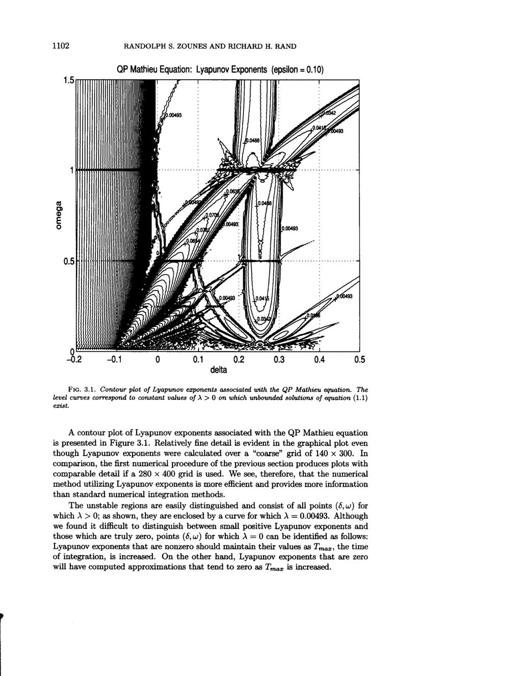
1 SIAM J. APPL. MATH. c 1998 Society for Industrial and Applied Mathematics Vol. 58, No. 4, pp , August TRANSITION CURVES FOR THE QUASI-PERIODIC MATHIEU EQUATION RANDOLPH S. ZOUNES AND RICHARD H. RAND Abstract. In this work we investigate an extension of Mathieu s equation, the quasi-periodic (QP) Mathieu equation given by ψ +[δ + ɛ (cos t + cos ωt)] ψ =0 for small ɛ and irrational ω. Of interest is the generation of stability diagrams that identify the points or regions in the δ-ω parameter plane (for fixed ɛ) for which all solutions of the QP Mathieu equation are bounded. Numerical integration is employed to produce approximations to the true stability diagrams both directly and through contour plots of Lyapunov exponents. In addition, we derive approximate analytic expressions for transition curves using two distinct techniques: (1) a regular perturbation method under which transition curves δ = δ(ω; ɛ) are each expanded in powers of ɛ, and () the method of harmonic balance utilizing Hill s determinants. Both analytic methods deliver results in good agreement with those generated numerically in the sense that predominant regions of instability are clearly coincident. And, both analytic techniques enable us to gain insight into the structure of the corresponding numerical plots. However, the perturbation method fails in the neighborhood of resonant values of ω due to the problem of small divisors; the results obtained by harmonic balance do not display this undesirable feature. Key words. quasi-periodic, Floquet theory, Hill s equation, Mathieu equation, perturbations, stability AMS subject classifications. 34, 34D, 34E, 34D08, 34D10, 34E10 PII. S Introduction. This work deals with a generalization of Hill s equation, a term which refers to any homogeneous, linear, second-order differential equation given by ẍ + f(t) x =0, where f(t) is a real periodic function in t. Motivated primarily by problems in mechanics and astronomy, and in part by the investigation of the stability of periodic motions in autonomous nonlinear systems, many results have been generated which collectively form Floquet theory (see Magnus and Winkler [18]). A special case of Hill s equation is Mathieu s equation, ẍ +(δ + ɛ cos t) x =0, the archetypal problem in parametric excitation in which an autonomous linear structure is driven by a periodic forcer. The stability or boundedness of solutions of Mathieu s equation as a function of parameter values (δ, ɛ) has been extensively examined and characterized in terms of stability transition curves that demarcate the boundaries of instability regions. They consist of one-dimensional curves in the δ-ɛ parameter Received by the editors May 17, 1996; accepted for publication (in revised form) March 9, 1997; published electronically May 11, Center for Applied Mathematics (CAM), Cornell University, Ithaca, NY (zounes@ cam.cornell.edu). Department of Theoretical and Applied Mechanics (T&AM), Cornell University, Ithaca, NY (rhr@cornell.edu). 1094

2 QUASI-PERIODIC MATHIEU EQUATION 1095 plane that separate points (δ, ɛ) for which at least one solution of Mathieu s equation is unbounded (unstable) from points for which all solutions are bounded (stable). A seemingly straightforward extension of Mathieu s equation, the quasi-periodic (QP) Mathieu equation given by (1.1) ψ +[δ + ɛ (cos t + cos ωt)] ψ =0, ω irrational, is investigated in this paper. Since the coefficient of ψ in (1.1) is QP but not periodic, Floquet theory is inapplicable, and qualitatively new difficulties absent from the analysis of Mathieu s equation are encountered. Numerical integration employing the Runge Kutta method of order 4 is used to generate stability charts graphical plots of points (δ, ω) in the δ-ω parameter plane for which all solutions of equation (1.1) are bounded as well as contour plots of Lyapunov exponents. In addition, two systematic techniques for generating approximate analytic expressions for the transition curves in the δ-ω parameter plane, which parallel those used for Mathieu s equation, are presented. The first technique is a regular perturbation method under which δ(ω; ɛ) is expanded in powers of ɛ. It is based on the conditions that (1) along transition curves, at least one solution of the QP Mathieu equation is bounded; and () transition curves bounding regions of instability in the δ-ɛ parameter plane emanate from points on the δ-axis at δ = 1 4 (a + bω), a,b Z, a set of points which is dense in the δ-axis. Although in good agreement for a wide range of parameter values, this technique fails in the neighborhood of resonant values of ω due to the problem of small divisors. The second technique assumes that bounded solutions along transition curves have the form ψ(t) = a=0 b= [A ab cos( a+bω t)+b ab sin( a+bω t)] and utilizes Hill s method of infinite determinants in conjunction with harmonic balance to derive implicit analytic expressions for the transition curves. This analytic technique delivers results consistent with those generated numerically, yet does not suffer from the small-divisor problem. A vast body of research directed toward the theory of ordinary differential equations with almost periodic coefficients has accumulated since the works of Bochner [] and Favard [9], evident from the extensive bibliographies of [6] and [10], in which hundreds of references are cited. Nonetheless, it has proved useful to examine the question of the boundedness of solutions of the QP Mathieu equation from the perspective of functional analysis. Specifically, the QP Mathieu equation is viewed as a (self-adjoint) QP Schrödinger operator on L (R) defined by ) Lψ = ( d ɛ (cos t + cos ωt) ψ = δψ, dt whose spectral properties provide information on the form and boundedness of associated solutions. Being interested in generating stability diagrams, we can identify the resolvent set of L, ρ(l), with regions of instability, and we can identify the absolutely continuous component of the spectrum, σac(l), with regions of stability. Furthermore, the following results hold.

3 1096 RANDOLPH S. ZOUNES AND RICHARD H. RAND 1. Pastur and Figotin show in [4] that up to a set of measure zero, the absolutely continuous component of the spectrum coincides with those values of δ, given fixed ɛ and fixed ω, for which the associated Lyapunov exponent is zero. Hence, we can identify regions of stability with the set of points for which the associated Lyapunov exponent vanishes.. As demonstrated by Johnson and Moser in [15], the winding number, which measures the average increase of the phase of any solution, is constant on ρ(l). If I is an open interval in the resolvent set, then the winding number W = W (δ) assumes a value of the form W (δ) 1 M = { 1 (j 1 + ωj ):j 1,j Z}, where M is the frequency module of the driving term (potential) of L. This result is significant in relation to the perturbation method discussed in this paper. As shown in [33], the winding number associated with the QP Mathieu equation can be expressed as (1.) W = δ + ɛ δ lim 1 T cos φ(t)(cos t + cos ωt) dt, T T 0 where φ(t) is the phase of a corresponding solution. Thus, we see that W = 1 (j 1 + ωj ) δ as ɛ 0 for points in the resolvent set, implying that the corresponding transition points on the δ-axis in the δ-ɛ parameter plane are 1 4 (j 1 + ωj ), j 1,j Z, as asserted above. 3. Suppose ω satisfies typical Diophantine conditions given in the paper by Moser and Pöschel []. If µ 1 M (minus a small set of exceptional values) and if ɛ/ δ is sufficiently small, then solutions of the QP Mathieu equation along transition curves (boundaries of instability regions) have the form ψ(t) = e iµt χ(t), χ Q(1,ω), where Q(1,ω) is the set of all QP functions with independent frequencies 1 and ω. This implies that solutions along transition curves are QP functions with independent frequencies 1 and ω, the form assumed by the method of harmonic balance. A major theme pertaining to the analysis of Schrödinger operators with almost periodic potentials is the tendency for the associated spectra of H to be Cantor sets, i.e., sets that are closed, have no isolated points, and whose complement is dense. Consider the quantum mechanical system Hψ = ) ( d dx + V (x) ψ = Eψ, with potential V (x) = n 1,n a n1,n exp[i(n 1 + n ω)x],

4 QUASI-PERIODIC MATHIEU EQUATION 1097 where ω = p/q with p, q relatively prime. If ω<1, V (x) has period πq and the usual analysis of periodic potentials shows that for small ɛ, the spectrum of H will have gaps about the points E k = 1 ( ) k, k =0, 1,,... 4 q Since p and q are relatively prime, k can be expressed as the linear combination k = n 1 q + n p for some n 1,n Z. Therefore, it is natural to suppose that when ω is irrational there is still a tendency for the spectrum of H to have gaps about the points E n1,n = 1 ( ) n1 q + n p = 1 4 q 4 (n 1 + n ω). Since these points are dense in R, the associated gaps in the spectrum will be dense, and the resulting spectrum will be a Cantor set, although one of nonzero Lebesgue measure depending on the coefficients a n1,n of the potential V (x). The first hint of this gap picture was in a paper by Dinaburg and Sinai [8]. We expect the stability diagrams of the QP Mathieu equation, therefore, to be quite intricate: a dense collection of instability regions stratifies the δ-ω parameter plane, leaving behind regions of stability with a Cantor-like structure. A 198 paper by Simon [9] provides an excellent review of the then recent literature on the one-dimensional Schrödinger equation with an almost periodic potential. Other important papers among scores include [15], [14], and [1], in which the rotation number (winding number) is used to extract properties of the spectrum, as mentioned above. In [31], Vrscay applies a regular perturbation method to the QP Mathieu equation in order to examine the irregular nature of the associated spectrum. Hofstadter [13] carries out an interesting analysis of a quantum mechanical system describing the two-dimensional motion of a crystal electron (Bloch electron) in a uniform magnetic field. He presents numerical results of the system s spectrum as a function of a parameter whose rationality or irrationality highly influences its nature. The graph of the spectrum, Hofstadter s butterfly, has a fine-grained structure similar to the stability charts of the QP Mathieu equation presented in this paper. Due in part to an incomplete, general theory of differential equations with almost periodic coefficients, and in part to the lack of communication between physicists and engineers, the determination of analytic expressions for transition curves in a parameter plane has received little attention in the literature. In a paper by Davis and Rosenblat [7], a multiple-scales technique is used to compute transition curves expressed in powers of ɛ for the QP Mathieu equation. Although calculations through only O(ɛ ) were performed, they claim to suppress small divisors by detuning off of resonances. Moreover, they speculate that transition curves emanate from the δ-axis in the δ-ɛ parameter plane from two families of points, namely, δ = 1 4 a,a=0, 1,,..., and δ = 1 4 (bω), b =0, 1,,... Our work, as well as that by Abel [1], indicates, however, that the appropriate location of transition points on the δ-axis in the δ-ɛ parameter plane is δ = 1 4 (a + bω),a,b Z. Other papers in which transition curves for QP systems are generated include those by Schweitzer [7] and Weidenhammer [3]. Schweitzer utilizes the results of Shtokalo given in [8] that provide conditions for the stability or instability of solutions to linear, QP systems. The conditions depend on the construction of a linear transformation, written as a formal series in powers of ɛ, that transforms the original QP system to one with constant coefficients. The stability

5 1098 RANDOLPH S. ZOUNES AND RICHARD H. RAND of solutions are inferred by examining the associated Hurwitz determinants of the new system, which Schweitzer uses to extract information about the transition curves. In [3], Weidenhammer applies a perturbation method to a nonlinear QP equation, and computes a number of analytic expressions for transition curves through O(ɛ ). From one last perspective, the QP Mathieu equation may be seen as a perturbation of an integrable Hamiltonian system. In this context, one is inclined to apply KAM theory or averaging-type methods to (1.1), as described in the recent book by Lochak and Meunier [17]. However, since equation (1.1) is linear, nondegeneracy conditions necessary for its application cannot be satisfied (i.e., there is no twist ). Hence, we do not pursue this line of investigation.. Numerical integration. Presented in this section are the graphical results of numerical investigations into the asymptotic behavior of the QP Mathieu equation. Numerical integration employing the Runge Kutta method of order 4 [3] is carried out to generate stability charts by integrating equation (1.1) forward in time over a grid of parameter values in the δ-ω parameter plane. To determine whether or not the solution associated with a given point (δ, ω) of the grid becomes unbounded with time (i.e., is unstable), two distinct procedures were implemented. The first procedure follows a standard methodology wherein the QP Mathieu equation is integrated for a preset length of time. At each step of the integration, the amplitude of the solution ψ(t) in the phase plane, (.1) r(t) = ψ(t) = ψ(t) + ψ(t), is calculated and used to determine whether or not the solution has grown without bound (is unstable) based on the following criteria: The solution ψ(t) of equation (1.1) is deemed unstable if, within a preset T max time units, its amplitude has increased by a factor of R. Otherwise, ψ(t) is said to be stable. It is worthwhile to remark that the quantities R and T max, which took on values 10 6 and 0000, respectively, are arbitrary and should be assigned according to the system or application at hand. Also, the stability of the system (i.e., of the zero solution) for a particular triplet (δ, ɛ, ω) is independent of initial conditions. Hence, the initial condition ψ 0 =0.001 and ψ 0 =0.001 was chosen arbitrarily and held fixed throughout the entire numerical procedure. The mutual dependence of R, T max, and ɛ on the numerical results can be made quantitative by applying a result given in section 3.10 of [5] to equation (1.1) rewritten as the first-order system (ẋ ) ( ) x (.) = A(t), ẏ y where A(t) is the matrix ( 0 (.3) A(t) = δ [1+ ɛ ] δ (cos t + cos ωt) ) δ. 0 (.4) Theorem.1. Every solution x(t) of equation (.) satisfies the double inequality ( t ) exp λ(α) dα t o x(t) x(t o ) ( t ) exp Λ(α) dα, t o

6 QUASI-PERIODIC MATHIEU EQUATION 1099 where λ(t) and Λ(t) are, respectively, the smallest and greatest characteristic roots (necessarily real) of the symmetric matrix H(t) = 1 [A(t)+AT (t)]. For the system defined by equations (.) and (.3), the characteristic roots of H(t) are λ(t) = ɛ ɛ cos t + cos ωt and Λ(t) = δ cos t + cos ωt, δ and the right-hand inequality reduces to (.5) x(t) x(t o ) e ɛ(t to)/ δ. For an R-fold increase in x(t) over a duration of time T max, equation (.5) implies that R exp(ɛt max / δ), or equivalently, ɛt max δ ln R. These expressions suggest that when ɛ is held fixed, comparable graphical results are achieved for combinations of T max and R that maintain the ratio, T max / ln R. In addition, whenever ɛ is decreased, more time is needed for an R-fold increase in x(t), indicating that the growth rates of unstable solutions diminish with ɛ. It is possible, therefore, that genuinely unstable solutions may be classified as stable if T max is chosen too small for a given ɛ. The second procedure for ascertaining the stability or instability of a given point (δ, ω) of the grid makes use of the fact that only rational numbers are realized on a computer. Let ω = p/q, where p and q are relatively prime integers. By rescaling time according to t = qτ and letting the prime denote differentiation with respect to τ, the QP Mathieu equation can be written as (.6) ψ + 4q [δ + ɛ (cos qτ + cos pτ)] ψ = 0, which now has a driving term with period π. If ψ 1 (τ) and ψ (τ) are the linearly independent normalized solutions of (.6) determined by the initial conditions, y 1 (0)=1, y (0)=0, y 1(0)=0, y (0)=1, then as discussed in [18], all solutions of (.6) are stable if and only if ψ 1 (π) < 1. As a result, equation (.6) needs to be integrated only over the interval τ [0,π], and no arbitrary conditions that deem solutions as stable or unstable are required. We see that this procedure is not only more efficient than the first, it is more accurate as well. We should remark, however, that the step size used in the numerical integration depends on q and was set to τ = π/(64q); this corresponds to 64 time steps per period of the cos t driver. Stability charts identifying points (δ, ω) in the δ-ω parameter plane for which all solutions of the QP Mathieu equation are bounded are presented in Figures.1 and.. The chart shown in Figure.1 took six months to produce, running in the background on a Sun SPARCstation 5, under the implementation of the first procedure (R =10 6 and T max = 0000), and was generated over a grid of points. The chart shown in Figure. took only one month to produce, running in the background on a Sun SPARCstation 5, under the implementation of the second procedure, and was generated over an grid of points. Although at the expense of much computational effort and time, the fine resolution of the figures reveals an intricate web of instability regions cutting across the parameter plane.

7

8

9

10 QUASI-PERIODIC MATHIEU EQUATION Perturbation method. For generating approximate analytic expressions for transition curves δ = δ(ɛ) in the δ-ɛ parameter plane, a regular perturbation method based on expansions in powers of ɛ (see [16], [3], [5], and [30]) has been very successful when applied to Mathieu s equation, (4.1) ẍ +(δ + ɛ cos t) x =0. The procedure is based on the result from Floquet theory that equation (4.1) can exhibit periodic solutions with period π or 4π if and only if the associated pair (δ, ɛ) of parameter values lies on a transition curve. As a consequence of this result, pairs of transition curves emanate from the δ-axis (ɛ =0)atδ = 1 4 a, a =0, 1,,...and bound tongue-like regions of instability in the δ-ɛ parameter plane. Under this perturbation method, one assumes that ɛ is small and expands δ(ɛ) and x(t) as follows: (4.) (4.3) δ(ɛ) =δ 0 + ɛδ 1 + ɛ δ +, x(t) =x 0 (t)+ɛx 1 (t)+ɛ x (t)+. Insertion of equations (4.) and (4.3) into (4.1) and equating coefficients of like powers of ɛ yields a sequence of differential equations from which the functions x i are determined. General expressions for the x i are obtained and forced to be periodic with period 4π by choosing the coefficients δ i accordingly. By independently setting x 0 (t) to sin( a t) and cos( a t), respectively, the two transition curves emanating from δ = 1 4 a are generated. A perturbation method similar to the one used on Mathieu s equation, with the objective of generating analytic expressions for the transition curves δ = δ(ω; ɛ) in the δ-ω parameter plane (fixed ɛ), may be applied to the QP Mathieu equation. As is done above, one assumes that ɛ is small and expands δ(ω; ɛ) in powers of ɛ: (4.4) δ(ω; ɛ) =δ 0 (ω)+ɛδ 1 (ω)+ɛ δ (ω)+. The corresponding solutions along the transition curves are expanded in powers of ɛ as well: (4.5) ψ(t) =ψ 0 (t)+ɛψ 1 (t)+ɛ ψ (t)+. Since ω is assumed to be irrational, the QP Mathieu equation cannot possess periodic solutions for any nonzero choice of ɛ. As a result, Floquet theory is inapplicable for providing a rigorous, clear-cut condition that distinguishes solutions along transition curves like having period π or 4π for Mathieu s equation for the QP Mathieu equation. Based on arguments presented above and in the next section, however, solutions along the transition curves are precisely those QP functions given by (4.6) ψ(t) = a=0 b= [ Aab cos ( a+bω t ) + B ab sin ( a+bω t )], where a 0 and b are integers. The perturbation method will yield solutions of the above form and generate analytic expressions for the transition curves if the following conditions are met. 1. Resonant terms are systematically removed from the differential equations for the ψ i. This condition, which is applied to similar problems utilizing perturbation theory, guarantees that the generated solution will be bounded.

11 1104 RANDOLPH S. ZOUNES AND RICHARD H. RAND. Transition curves bounding regions of instability in the δ-ɛ parameter plane emanate from points on the δ-axis at δ 0 = 1 4 (a+bω),a,b Z. This condition, as discussed above in the Introduction, is based on results by Johnson and Moser [15]. Before proceeding with the perturbation method defined by equations (4.4) and (4.5), we must first address the problem of small divisors characteristic of systems with two or more frequencies, and find conditions for the convergence of the expansions in ɛ. One can think of the QP Mathieu equation as a system of three linear oscillators having natural frequencies δ,1,andω with weak, nonlinear coupling. If the coupling is not too strong, the associated trajectories lie on a 3-torus in phase space, and the dynamics can be described in terms of a triplet of phase angles. The series expansion (4.5) for ψ(t), then, will contain terms of the form (see [11]) where A m cos(m ωt) + B m ω m sin(m ωt), m ω m ω = m 1 δ + m 1 + m 3 ω. Since the m s can take on negative values, there may be combinations of them such that m ω 0 as m = m 1 + m + m 3, and the series for ψ(t) need not converge. In two papers written by Moser in the 1960s [19], [0], a perturbation method for QP solutions with origins in papers by Kolmogorov and Arnold is described. As applied to the QP Mathieu equation, the following result is given. Theorem 4.1. Assume that δ 0, 1, and ω are rationally independent and satisfy the infinitely many inequalities, (4.7) j δ 0 + a 1 + b ω c ( a + b ) γ, for all integers a and b with a + b > 0 and for j =0, 1, ; the constants γ and c are fixed. Then there exists an analytic function in ɛ, δ(ω; ɛ) = δ 0 (ω)+ɛδ 1 (ω)+ɛ δ (ω)+, such that the QP Mathieu equation possesses a QP solution with basic frequencies 1 and ω. Forγ>1 and for almost all ω, such a constant c can be found. A QP function with basic frequencies 1 and ω is a special case of (4.6); hence, the analytic function δ(ω; ɛ) given in the theorem must be an expression for a transition curve. The Diophantine condition given by (4.7) can be seen as three independent conditions, one for each value of j. Ifj = 0, then (4.7) fails whenever ω is rational; there will be terms in the expansion for δ that have vanishing denominators resulting in a divergent series. If either j =1orj =, then (4.7) fails whenever ± δ 0 = 1 a + bω

12 QUASI-PERIODIC MATHIEU EQUATION 1105 for integers a and b that are not simultaneously zero, or equivalently, δ 0 = 1 4 (a + bω). Hence, we see that the transition points from which pairs of transition curves in the δ- ɛ parameter plane emanate are resonant values of the natural frequency. In addition, since ω is assumed to be irrational, the set of transition points T = { 1 4 (a + bω) : a, b Z} has no repeated elements, given that a is nonnegative. Consequently, the pair of transition curves emanating from the transition point δ = 1 4 (a+bω) can be identified with the ordered pair, (a, b). This exactly parallels the identification of ordered pairs of integers with spectral gaps in the resolvent set of L (cf. [15]). From another viewpoint, the elements of T can be seen as the zeroth-order (ɛ =0) approximations to the transition curves in the δ-ω parameter plane. For a given pair (a, b) of integers, a curve with equation δ = 1 4 (a + bω) the coalescence of the two associated transition curves emanates from the δ-axis (ω =0)atδ = 1 4 a. When ɛ is increased, the curve fattens into a region of instability. Since an infinite number of such curves emanate from the δ-axis at δ = 1 4 a, one for each b Z, we expect to find an infinite number of instability regions fanning out from this point. The most prominent region of instability is vertical and corresponds to b = 0. As b is increased, the associated regions diminish in width and fan out at smaller angles with respect to the δ-axis. Numerical results presented in the previous sections support this description of instability regions in the δ-ω parameter plane. Proceeding formally with the perturbation method, equations (4.4) and (4.5) are substituted into the QP Mathieu equation (1.1). Equating coefficients of like powers of ɛ yields the following sequence of differential equations from which the ψ i can be determined recursively: O(ɛ 0 ): ψ0 + δ 0 ψ 0 =0, O(ɛ 1 ): ψ1 + δ 0 ψ 1 = δ 1 ψ 0 (cos t + cos ωt)ψ 0, O(ɛ ): ψ + δ 0 ψ = δ 1 ψ 1 δ ψ 0 (cos t + cos ωt)ψ 1,. O(ɛ i ): i 1 ψi + δ 0 ψ i = δ i j ψ j (cos t + cos ωt)ψ i 1, j=0 Expressions δ i (ω) which describe the transition curves are determined by systematically removing resonant terms from the differential equations for the ψ i,as is done for Mathieu s equation. Since the forcing term ɛ (cos t + cos ωt) in the QP Mathieu equation is an even function, each transition curve from a given pair can be independently generated by separately considering the initial conditions (i) ψ(0)=0 ψ i (0)=0, i =0, 1,,..., (ii) ψ(0)=0 ψ i (0)=0, i =0, 1,,... For case (i), the solution along one transition curve is odd, implying we set ( ) a + bω ψ 0 (t) = sin t ;.

13 1106 RANDOLPH S. ZOUNES AND RICHARD H. RAND and for case (ii), the solution along the other transition curve is even and we set ( ) a + bω ψ 0 (t) = cos t. With the aid of the symbolic computation system Maple [4], the above process was systematically repeated to generate the analytic expressions δ(ω; ɛ) = 1 4 (a + bω) + ɛδ 1 (ω)+ɛ δ (ω)+ for a variety of transition curves. Results through O(ɛ 3 ) are presented below. For each pair of transition curves, the first expression corresponds to the transition curve generated from ψ 0 (t) = sin( a+bω t), and the second corresponds to the transition curve generated from ψ 0 (t) = cos( a+bω t). The case δ 0 = 0 has a single transition curve generated from ψ 0 (t) =1. Case δ 0 =0: a =0and b =0. (4.8) a=0 δ = 1 ɛ ( 1+ 1 ω ) + O(ɛ 4 ). Case δ 0 = 1 4 ω : a =0and b =1. (4.9) δ = 1 4 ω + 1 ɛ 1 8 ɛ ( 1+3ω ) ω (1 ω ) 1 ɛ ( 3 16 ω 6 + ω 4 ω +1 ) 3 ( ω 1) ( ω +1) ω 4 + O(ɛ 4 ), (4.10) δ = 1 4 ω 1 ɛ 1 8 ɛ ( 1+3ω ) ω (1 ω ) + 1 ɛ ( 3 16 ω 6 + ω 4 ω +1 ) 3 ( ω 1) ( ω +1) ω 4 + O(ɛ 4 ). Case δ 0 = 1 4 : a =1and b =0. (4.11) δ = ɛ a=1 ɛ ( 3+ω ) 1 ω + 1 ɛ ( 3 ω 6 ω 4 + ω +16 ) 3 ( ω 1) ( ω +1) ω + O(ɛ 4 ), (4.1) δ = ɛ ɛ ( 3+ω ) 1 ω 1 ɛ ( 3 ω 6 ω 4 + ω +16 ) 3 ( ω 1) ( ω +1) ω + O(ɛ 4 ). Case δ 0 = 1 4 (1 + ω) : a =1and b =1. (4.13) δ = 1 4 ( ω +1) 1 ɛ ( ω + ω +1 ) ω ( ω +1)(ω +) + O(ɛ4 ), (4.14) δ = 1 4 ( ω +1) + 3 ɛ ( ω +3ω +1 ) ω ( ω +1)(ω +) + O(ɛ4 ).

14 Case δ 0 = 1 4 (1 ω) : a =1and b = 1. (4.15) QUASI-PERIODIC MATHIEU EQUATION 1107 δ = 1 4 (1 ω ) + 1 ɛ ( ω ω +1 ) ω ( ω 1) (ω ) + O(ɛ4 ), (4.16) δ = 1 4 (1 ω ) 3 ɛ ( ω 3 ω +1 ) ω ( ω 1) (ω ) + O(ɛ4 ). A plot displaying a variety of transition curves along with those given in equations (4.8) (4.16) is presented in Figure 4.1. There is good agreement with the results generated numerically in the sense that predominant regions of instability are clearly coincident. Moreover, the perturbation results contain finger-like regions of instability that fan out from the δ-axis near δ = 0 and δ = 1 4. However, the expressions for the 1 transition curves are not valid in neighborhoods of ω = 0, 3, 1, 3, 1, 3,, and 3, since there are terms that have vanishing denominators at these resonant values. Consequently, these portions of the transition curves are omitted as is evident in Figure 4.1. The largest regions of instability, as shown in the figures produced both numerically and via the perturbation method, are those that lie in the neighborhood of the curves δ = 1 4 ω (a =0,b= 1) and δ = 1 4 (a =1,b= 0) and have a width of O(ɛ). Each represents a :1 resonance between a respective driving frequency (ω or 1) and the natural frequency of the unperturbed system, δ. One can see, in addition, finger-like regions of instability, though smaller, corresponding to other pairs of integers, (a, b). An interesting question arises: how does one identify the predominant regions of instability? A trigonometric expansion of the forcing term in each of the differential equations for the ψ i and an examination of high-order calculations indicate that the value n = a + b determines the relative order of importance. For a given pair of transition curves, the two coincide through O(ɛ n 1 ). Consequently, the width of the associated region of instability is O(ɛ n ), and the majority of such regions are merely curves of stability. Therefore, the most noticeable and interesting behavior in the δ-ω parameter plane occurs near δ = 0 and δ = 1 4 (a = 0 and a = 1, respectively). In principle, we could have obtained higher-order truncations, but additional resonances would have appeared. A perturbation method based on expansions in powers of ɛ is problematic for generating stability transition curves in the δ-ω parameter plane. Fortunately, the analytic technique presented in the next section does not suffer from divergence problems near resonant values of ω. 5. Hill s determinant and harmonic balance. Another technique available for generating analytic expressions for the transition curves of Mathieu s equation (4.1) involves the use of Hill s infinite determinants (see [16], [18], and [3]). Under this method, the bounded solutions x(t) along the transition curves, known to be periodic with period π or 4π, are represented by the Fourier series, (5.1) [ x(t) =A 0 + Ak cos( k t)+b k sin( k t)]. k=1 Substituting the above expression into Mathieu s equation and matching terms with the same harmonics (i.e., harmonic balance) leads to an infinite set of linear, homogeneous equations for the coefficients {A k,b k }. In order for x(t) to be nontrivial, the infinite (or Hill s) determinant of the associated coefficient matrix must vanish. It is

15 1108 RANDOLPH S. ZOUNES AND RICHARD H. RAND QP Mathieu Equation: Perturbation Method (epsilon = 0.10) omega delta Fig Transition curves for the QP Mathieu equation (1.1) as determined by the perturbation method, ɛ =0.10. The regions around resonant values of ω have been omitted. this condition that implicitly specifies the transition curves in the δ-ɛ parameter plane for Mathieu s equation. A similar technique utilizing Hill s method of infinite determinants, with the objective of determining analytic expressions for the transition curves in the δ-ω parameter plane (fixed ɛ), proved to be successful when applied to the QP Mathieu equation. It revolves around the assertion that solutions along transition curves have the form given by equation (4.6), specifically, ψ(t) = a=0 b= [ Aab cos ( a+bω t ) + B ab sin ( a+bω t )]. Strong motivation for the above assertion is made when ω is restricted to rational values: ω = p/q, where p and q are relatively prime, positive integers. Seemingly, there is no physical effect stemming from the irrationality of ω since an arbitrarily small change in ω would make it rational. Moreover, an irrational number can be approx-

16 QUASI-PERIODIC MATHIEU EQUATION 1109 imated by a rational number to any degree of accuracy. With the above restriction imposed on ω, the QP Mathieu equation becomes the following Hill s equation: (5.) ψ +[δ + ɛ (cos t + cos p q t)] ψ =0. Assuming ω<1, the driving term ɛ(cos t + cos p q t) has period T =πq. According to Floquet theory, Hill s equation delivers periodic solutions with period T or T only if the associated parameter values lie on a transition curve. Hence, along a transition curve, the solution ψ(t) is represented by the following Fourier series: (5.3) ψ(t) =A 0 + k=1 [A k cos( kq t)+b k sin( kq t) ]. Since q and p are relatively prime, a theorem in Herstein s text [1] states that any integer k can be expressed as the linear combination k = aq + bp for some a, b Z. As a result, the set of integers can be put into a one-to-one correspondence with the following set of ordered pairs of integers: where Z P, P = {(a, b) Z Z : k = aq + bp, k Z}. Ordered pairs that yield the same integer are identified and defined to be in the same equivalence class. Hence, the above correspondence is actually between Z and the set of equivalence classes. The Fourier series (5.3) can then be expressed as ψ(t) = P [ A ab cos( aq+bp q t) + B ab sin( aq+bp q t) ] (5.4) = P [ Aab cos( a+bω t) + B ab sin( a+bω t) ], in the form of the assertion given by equation (4.6). The strongest argument for solutions along transition curves having the form given by equation (4.6), however, is derived from results pertaining to Schrödinger operators. As mentioned above in the Introduction, if ω satisfies typical Diophantine inequalities given in [] and if ɛ/ δ is sufficiently small, then the QP Mathieu equation has a solution along a transition curve given by (5.5) ψ 1 (t) =e iµt χ 1 (t), where χ 1 Q(1,ω) and µ = 1 (j 1 + ωj ) for some j 1,j Z. Being a QP function, χ 1 can be represented by the two-frequency Fourier series (5.6) χ 1 (t) = k 1,k C k e i(k1+ωk)t. Therefore, inserting the expression for µ and (5.6) into (5.5) and rewriting, we find that ψ 1 (t) can be expressed as ψ 1 (t) = k 1,k C k e i[(k1+ 1 j1)+ω(k+ 1 j)]t,

17 1110 RANDOLPH S. ZOUNES AND RICHARD H. RAND equivalent to the form given by equation (4.6). Without loss of generality, assume that solutions along the transition curves of the QP Mathieu equation are given by (5.7) ψ(t) = a=0 b= A ab cos( a+bω t). This simplification allows us to independently generate each transition curve of a given pair; the determination of the second transition curve is accomplished by assuming that (5.8) ψ(t) = a=0 b= B ab sin( a+bω t) and follows an identical analysis. Substituting equation (5.7) for ψ(t) into the QP Mathieu equation and simplifying yields (5.9) a=0 b= [ cos( a+bω t) A a,b (δ 1 4 (a + bω) ) ] + ɛ (A a+,b + A a,b + A a,b+ + A a,b ) =0. Equating each of the coefficients of cos( a+bω t) to zero which is equivalent to matching terms with the same harmonics results in the following infinite set of linear, homogeneous equations for the {A a,b }: (5.10) A a,b [δ 1 4 (a + bω) ]+ ɛ [A a+,b + A a,b + A a,b+ + A a,b ]=0. In order for ψ(t) to be a nontrivial solution of the QP Mathieu equation (1.1), the infinite determinant of the associated coefficient matrix, C, for the linear system defined by equation (5.10) must vanish. Assuming that the determinant exists, transition curves for the QP Mathieu equation are implicitly given by (5.11) det(c) =0, where det(c) is a function of ɛ, δ, and ω. To assure convergence of the infinite determinant, divide equation (5.10) through by (5.1) γ a,b = δ 1 4 (a + bω) ; this results in the new linear system, (5.13) A a,b + ɛ (A a+,b + A a,b + A a,b+ + A a,b )=0. γ a,b Before we can proceed, it is necessary to show that the infinite determinant of the coefficient matrix exists. According to Theorem.7 from Magnus and Winkler [18], determinants of Hill s type converge. Definition 5.1. Given a matrix A =(a ij ), the determinant is said to be of Hill s type if it satisfies the condition a ij δ ij <, ij

18 QUASI-PERIODIC MATHIEU EQUATION 1111 where δ ij = { 0 if i j, 1 if i = j. The determinant of the coefficient matrix, C, is readily seen to be of Hill s type, and hence, convergent. Indeed, (5.14) since C ij δ ij = ɛ 1 γ ij ab ab < (5.15) γ ab = O(a + b ). In practice, approximate expressions for det(c) are obtained by expressing solutions ψ of the QP Mathieu equation along transition curves as the following finite sums: (5.16) or (5.17) ψ(t) = ψ(t) = N N a=1 b= N N N a=1 b= N A ab cos( a+bω t)+ B ab sin( a+bω t)+ N A 0b cos( bω t) b=0 N B 0b sin( bω t). Increasing N yields better approximations to the transition curves, but the dimension of the coefficient matrix becomes geometrically larger, thereby making the evaluation of its determinant progressively harder. For example, if (5.16) is used as an approximate solution of the QP Mathieu equation, the dimension of C is N +N +1. In the case N = 4, the coefficient matrix has dimension 41. Although the analysis was facilitated by putting C in upper triangular form, the analytic evaluation of det(c) and the generation of graphical plots took an hour when Maple was executed on a Sun SPARCstation 10. Approximate analytic expressions for det(c) were obtained for the cases N = 1,, 3, and 4. For each N, two expressions for det(c) one corresponding to the coefficient matrix of the sine-series solution (5.17) and one corresponding to that of the cosine-series solution (5.16) were independently generated. The locus of points (δ, ɛ, ω) for which either expression equals zero comprises the set of transition curves at the given order of approximation. Graphical results for cases N = 1 and N =4 are presented in Figures 5.1 and 5., and analytic expressions for det(c), N = 1, are given below. Individual curves were extracted by setting factors of the expressions for det(c) to zero. Case N =1 sine-series solution: det(c) =(ɛ 4 δ +1) ( ω 4 δ +ɛ ) (5.18) ( 4 δ 1 ω ω )( ω +ω +4δ 1 ) ; cosine-series solution: det(c) =4δ (ɛ +4δ 1) ( ω 4 δ ɛ ) (5.19) ( 16 ɛ ω +1 8δ 8 ω δ +16δ + ω 4). b=1

19

20

21 1114 RANDOLPH S. ZOUNES AND RICHARD H. RAND 1. Regions of instability predictably get thinner and recede into the δ-axis as µ is increased.. It appears that high-order regions of instability are more affected by damping than low-order ones. In other words, the fine detail of the stability charts is lost even for small µ. 3. The regions of instability emanating from around δ = 1 4 eventually disappear as µ is increased. In fact, equation (5.1) predicts that the O(ɛ) region disappears when µ > 1 ɛ. In contrast, equation (5.) suggests that the region of instability centered on the curve δ = 1 4 ω will persist, at least for sufficiently small values of ω. 6. Discussion. Two analytic techniques for generating transition curves in the δ-ω parameter plane for the QP Mathieu equation were presented in the previous two sections. The first technique, a regular perturbation method, approximates transition curves δ = δ(ω; ɛ) by expansions in powers of ɛ. Although the perturbation method delivers results in good agreement with those generated numerically, it suffers from the small-divisor problem whereby the expansion of δ(ω; ɛ) is not valid near resonant values of ω. Moser s theorem illuminates the nature of the problem: by expressing δ(ω; ɛ) as a power series in ɛ, we are building into it divergence problems in the neighborhoods of resonant values of ω that do not satisfy the Diophantine condition (4.7). The perturbation method, therefore, is an inappropriate technique for generating graphical plots of the transition curves in the δ-ω parameter plane. The second technique, based on harmonic balance, utilizes Hill s method of infinite determinants for generating implicit analytic expressions for the transition curves in the δ-ω parameter plane. Harmonic balance delivers results in excellent agreement with those generated numerically yet does not suffer from the small-divisor problem. Moreover, it is directly applicable when dissipation is present in the system. The following question arises: in relation to harmonic balance, what is the source of the nonuniform convergence found in the perturbation method? The answer can be seen by examining a simple model that displays similar characteristics. Consider the toy problem, chosen because of its similarity to the expressions generated by the harmonic balance analysis, for which a perturbation solution is sought: ( δ 1 )(δ 14 ) (6.1) 4 ω = ɛ. In seeking a perturbation solution, expand δ = δ(ω; ɛ) in a power series in ɛ: (6.) δ(ω; ɛ) = δ 0 (ω) + ɛδ 1 (ω) +. Substituting (6.) into (6.1) and collecting terms gives the following perturbation solution to the toy problem: (6.3) δ(ω; ɛ) = ω ɛ +. Equation (6.3) is singular at ω = ±1 in a manner similar to the perturbation solutions of the QP Mathieu equation. We see, therefore, that the failure of the perturbation method is due to the assumed form of the solution: the expansion of δ(ω; ɛ) inpowers of ɛ is inappropriate for the problem defined by equation (6.1).

22 QUASI-PERIODIC MATHIEU EQUATION 1115 REFERENCES [1] J. M. Abel, On an almost periodic Mathieu equation, Quart. Appl. Math., 8 (1970), pp [] S. Bochner, Homogeneous systems of differential equations with almost periodic coefficients, J. London Math. Soc., 8 (1933), pp [3] R. L. Burden and J. D. Faires, Numerical Analysis, 3rd ed., Prindle, Weber & Schmidt, Boston, MA, [4] B. W. Char, K. O. Geddes, G. H. Gonnet, B. L. Leong, M. B. Monagan, and S. M. Watt, Maple V (Symbolic Computation System), Waterloo Maple Publishing, Waterloo, ON, Canada, [5] L. Cesari, Asymptotic Behavior and Stability Problems in Ordinary Differential Equations, nd ed., Springer-Verlag, New York, [6] C. Corduneanu, Almost Periodic Functions, nd ed., Chelsea, New York, [7] S. H. Davis and S. Rosenblat, A quasiperiodic Mathieu Hill equation, SIAM J. Appl. Math., 8 (1980), pp [8] E. I. Dinaburg and Y. G. Sinai, The one-dimensional Schrödinger equation with a quasiperiodic potential, Funk. Anal. i. Pril., 9 (1975), pp [9] J. Favard, Sur les équations différentielles à coefficients presque-périodiques, Acta Math., 51 (197), pp [10] A. M. Fink, Almost Periodic Differential Equations, Springer-Verlag, New York, [11] H. Haken, Advanced Synergetics: Instability Hierarchies of Self-Organizing Systems and Devices, Springer-Verlag, New York, [1] I. N. Herstein, Topics in Algebra, nd ed., John Wiley & Sons, New York, [13] D. R. Hofstadter, Energy levels and wave functions of Bloch electrons in rational and irrational magnetic fields, Phys. Rev. B, 14 (1976), pp [14] R. Johnson, Cantor spectrum for the quasi-periodic Schrödinger equation, J. Differential Equations, 91 (1991), pp [15] R. Johnson and J. Moser, The rotation number for almost periodic potentials, Commun. Math. Phys., 84 (198), pp [16] D. Jordan and P. Smith, Nonlinear Ordinary Differential Equations, nd ed., Clarendon Press, Oxford, UK, [17] P. Lochak and C. Meunier, Multiphase Averaging for Classical Systems, Springer-Verlag, New York, Translated by H. S. Dumas. [18] W. Magnus and S. Winkler, Hill s Equation, John Wiley & Sons, New York, [19] J. Moser, Combination tones for Duffing s equation, Comm. Pure Appl. Math., 18 (1965), pp [0] J. Moser, On the theory of quasiperiodic motions, SIAM Review, 8 (1966), pp [1] J. Moser, An example of a Schrödinger equation with almost periodic potential and nowhere dense spectrum, Comm. Math. Helv., 56 (1981), pp [] J. Moser and J. Pöschel, An extension of a result by Dinaburg and Sinai on quasi-periodic potentials, Comm. Math. Helv., 59 (1984), pp [3] A. H. Nayfeh and D. T. Mook, Nonlinear Oscillations, John Wiley & Sons, New York, [4] L. Pastur and A. Figotin, Spectra of Random and Almost-Periodic Operators, Springer- Verlag, New York, [5] R. H. Rand, Computer Algebra in Applied Mathematics: An Introduction to MACSYMA, Pitman, Boston, [6] R. H. Rand, Topics in Nonlinear Dynamics with Computer Algebra, Gordon and Breach, Langhorne, PA, [7] V. G. Schweitzer, Zur stabilität eines parametererregten schwingers, Z. Angew. Math. Mech., 46 (1966), pp. T134 T136. [8] I. Z. Shtokalo, Linear Differential Equations with Variable Coefficients, Hindustan Publishing Company, Delhi, India, [9] B. Simon, Almost periodic Schrödinger operators: A review, Adv. Appl. Math., 3 (198), pp [30] J. Stoker, Nonlinear Vibrations in Mechanical and Electrical Systems, John Wiley & Sons, New York, [31] E. R. Vrscay, Irregular behaviour arising from quasiperiodic forcing of simple quantum systems: Insight from perturbation theory, J. Phys. A, 4 (1991), pp. L463 L468. [3] F. Weidenhammer, Nicht-lineare schwingungen mit fast-periodischer parametererregung, Z. Agnew. Math. Mech., 61 (1981), pp [33] R. Zounes, An Analysis of the Nonlinear Quasiperiodic Mathieu Equation, Ph.D. Thesis, Cornell University, Ithaca, NY, 1997.