Math 233 Calculus 3 - Fall 2016

Transcription

1 Math 233 Calculus 3 - Fall 2016

2 Three-Dimensional Coordinate Systems THREE-DIMENSIONAL COORDINATE SYSTEMS Definition. R 3 means By convention, we graph points in R 3 using a right-handed coordinate system. Righthanded means: Question. For two points P 1 = (x 1, y 1, z 1 ) and P 2 = (x 2, y 2, z 2 ) in R 3, what is the distance between P 1 and P 2? Question. What is the equation of a sphere of radius r centered at the point (h, k, l)?

3 Circle the right-handed coordinate systems THREE-DIMENSIONAL COORDINATE SYSTEMS

4 THREE-DIMENSIONAL COORDINATE SYSTEMS Example. (# 10) Find the distance from (4, 2, 6) to each of the following: a. The point (9, 1, 4) b. The xy-plane (where z = 0) c. The xz-plane d. The x-axis

5 THREE-DIMENSIONAL COORDINATE SYSTEMS Example. Describe the region (and draw a picture). a. z 2 b. x 2 + z 2 9 c. x 2 + y 2 + z 2 > 2z

6 12.6 QUADRIC SURFACES 12.6 Quadric Surfaces Match the equation to the graph using only your brain (no graphing software). Check your answer with graphing software. A. B. C. D. E. F. G. H. I. 1. x 2 + z 2 = x 2 + 4y 2 + 9z 2 = x 2 y 2 + z = 0 4. x 2 + y 2 + z = 0 5. x y 6. x 2 4y 2 + z 2 = 0 7. x 2 + y 2 z 2 = 1 8. x 2 y 2 + z 2 = 1 9. x 2 + y 2 + z 2 = x

7 12.2 VECTORS 12.2 Vectors Definition. A vector is a quantity with direction and magnitude (length). Vectors are usually drawn with arrows. Two vectors are considered to be the same if: Example. Which pairs of vectors are equivalent? Definition. A scalar is another word for. A scalar does not have a direction, in contrast to a vector.

8 12.2 VECTORS Vector addition: Draw a + b Multiplication of scalars and vectors: Draw 2 a and 3 a

9 12.2 VECTORS Note. In 2-dimensions, if we place the initial point of a vector a at the origin, and find its terminal point (a 1, a 2 ), then another way of representing the vector is using angle bracket notation: The numbers a 1, a 2 are called the of the vector. Example. The two equivalent vectors drawn above can both be written as <, >. Note. In 3-d, vectors have 3 components < a 1, a 2, a 3 >.

10 12.2 VECTORS Question. What are the components of the vector AB that starts at a point A = (3, 1) and ends at a point B = ( 2, 5)? Note. In general, the components of the vector that starts at a point A = (x 1, y 1 ) and ends at a point B = (x 2, y 2 ) are:

11 12.2 VECTORS Note. Given two vectors a =< a 1, a 2 > and b =< b 1, b 2 >, and a scalar c a + b = a b = c a = Similarly, for three-dimensional vectors a =< a 1, a 2, a 3 > and b =< b 1, b 2, b 3 >, a + b = a b = c a =

12 12.2 VECTORS Properties of vectors: 1. Addition is commutative 2. Addition is associative 3. Additive identity (the zero vector) 4. Additive inverses 5. Distributive property 6. Distributive property 7. Associativity of scalar multiplication 8. Multiplicative identity Definition. The length of a vector v =< v 1, v 2 > is v = Definition. The length of a vector w =< w 1, w 2, w 3 > is w = Note. The length of a vector is also called:

13 12.2 VECTORS Definition. A unit vector is a vector Question. How can we rescale any vector to make it a unit vector? (Rescale means multiply by a scalar.) Note. Rescaling a vector to make it a unit vector is also called normalizing the vector. Example. Find a unit vector that has the same direction as < 5, 1, 3 >. Definition. i =< 1, 0 >, j =< 0, 1 > are the in 2-dimensions. Definition. The standard basis vectors in 3-dimensions are:

14 12.2 VECTORS Review. Vectors can be represented with Example. Which arrow(s) represent(s) the vector < 2, 1 >? Example. Write < 2, 1 > as a sum of multiples of standard basis vectors.

15 12.2 VECTORS Example. (#41 from book) Find the unit vectors that are parallel to the tangent line to y = x 2 at (2, 4).

16 12.2 VECTORS Example. The 2-d vector v has magnitude 9 and makes an angle of 5π 6 x-axis. Find the components of v and write v in terms of i and j. with the positive

17 12.2 VECTORS Example. Two forces act as shown. Find the magnitude of the resultant force and the angle it makes with the positive x-axis.

18 12.2 VECTORS Example. Spiderman is suspended from two strands of spider silk as shown. Find the tension in each strand of spider silk. (You will need some additional information.)

19 12.2 VECTORS Question. Is there a difference between 0 and 0? Question. There are two definitions of vector addition: the vector definition and the component definition. Why are they the same?

20 12.3 DOT PRODUCT 12.3 Dot Product Definition. If a =< a 1, a 2, a 3 > and b =< b 1, b 2, b 3 >, then the dot product of a and b is given by a b = Question. Is a b a vector or a scalar? Note. Dot product satisfies the following properties: 1. Commutative Property: 2. Distributive Property: 3. Associative Property: 4. Multiplication by 0: 5. Relationship between dot product and norm:

21 12.3 DOT PRODUCT Definition. Dot product can also be defined in terms of magnitudes and norms: Question. If θ is the angle between a and b, what is cos(θ) in terms of the dot product? Question. Why are the two definitions of dot product the same?

22 Example. (# 11 and 12) If u is a unit vector, find u v and u w DOT PRODUCT

23 12.3 DOT PRODUCT Example. (# 31) Find the acute angle between y = x 2 and y = x 3 at their intersection point at (1, 1). Example. (#13) (a) Show that i j = j k = k i = 0 (b) Show that i i = j j = k k = 1

24 Example. (#27) Find a unit vector that is orthogonal to both i + j and i + k DOT PRODUCT

25 12.3 DOT PRODUCT Scalar and vector projections Definition. The scalar projection of b onto a is given by comp a b = Definition. The vector projection of b onto a is given by proj a b =

26 12.3 DOT PRODUCT Example. (#42) Find the scalar and vector projections of b =< 2, 3, 6 > onto a =< 5, 1, 4 >

27 12.3 DOT PRODUCT Definition. The work done by a constant force F moving an object along a vector D is the component of F in the direction of D, times the distance D. Question. How can we write work in terms of the dot product? Example. (# 51) A sled is pulled along a level path through snow by a rope. A 30-lb force acting at an angle of 40 above the horizontal moves the sled 80 ft. Find the work done by the force. (Round your answer to the nearest whole number.)

28 12.3 DOT PRODUCT Definition. The direction angles are the angles that a vector makes with the positive x, y, and z-axes. Example. Find the direction angles α, β, and γ of the vector v =< 3, 5, 4 > Find cos 2 α + cos 2 β + cos 2 γ. Why is this sum such a nice number?

29 12.3 DOT PRODUCT Extra Example. (# 53) Use scalar projection to show that the distance from a point P 1 (x 1, y 1 ) to the line ax + by + c = 0 is ax 1 + by 1 + c a2 + b 2 Use this formula to find the distance from the point ( 2, 3) and the line 3x 4y + 5 = 0.

30 12.3 DOT PRODUCT Extra Example. (# 61) Prove the Cauchy-Schwarz Inequality: a b a b

31 12.3 DOT PRODUCT Extra Example. (# 62) Prove the Triangle Inequality, which states that a + b a + b Hint: Use the fact that a + b 2 = ( a + b) ( a + b)

32 12.4 CROSS PRODUCTS 12.4 Cross Products Definition. The cross-product of two vectors a =< a 1, a 2, a 3 > and b =< b 1, b 2, b 3 > is given by: a b =

33 12.4 CROSS PRODUCTS Example. Compute a cross product: for a =< 1, 2, 3 > and b =< 5, 1, 10 >, find a b.

34 12.4 CROSS PRODUCTS Theorem. The vector a b is perpendicular to both a and b. Note that the direction of a b is given by the right hand rule:

35 12.4 CROSS PRODUCTS Theorem. If θ is the angle between a and b, with 0 θ π, then a b = a b sin θ Corollary. Two nonzero vectors a and b are parallel if and only if a b = 0.

36 12.4 CROSS PRODUCTS Example. For the two vectors shown, find a b and determine whether a b is directed into the page of out of the page.

37 12.4 CROSS PRODUCTS Review. The cross-product of two vectors a and b is defined as: or as Question. How can you use cross product to: find a vector perpendicular to two vectors? determine if two vectors are parallel?

38 Example. Find a unit vector orthogonal to both i + j and i + k CROSS PRODUCTS

39 12.4 CROSS PRODUCTS Example. Use the cross product to write the area of the parallelogram in terms of a and b. Example. Use the cross product to write the volume of the parallelpiped in terms of a, b, and c.

40 12.4 CROSS PRODUCTS Example. (# 30) Find the area of the triangle with vertices P(0, 0, 3), Q(4, 2, 0), and R(3, 3, 1).

41 12.4 CROSS PRODUCTS Example. Are these three vectors coplanar? u = 2 i + 3 j + k v = i j w = 7 i + 3 j + 2 k

42 12.4 CROSS PRODUCTS True or False 1. a b is a scalar. 5. a b = b a 2. a a = ( a b) c = a ( b c) 3. For a, b 0, if a b = 0 then a = b. 7. a ( b + c) = a b + a c 4. i j = k

43 12.4 CROSS PRODUCTS

44 12.4 CROSS PRODUCTS Extra Example. (#44) 1. Find all vectors v such that < 1, 2, 1 > v =< 3, 1, 5 >. 2. Explain why there is no vector v such that < 1, 2, 1 > v =< 3, 1, 5 >.

45 12.5 LINES AND PLANES 12.5 Lines and Planes Example. Is the line through ( 4, 6, 1) and ( 2, 0, 3) parallel to the line through (10, 18, 4) and (5, 3, 14)? What is the equation of the line through the origin, that is parallel to the line through ( 4, 6, 1) and ( 2, 0, 3)? What is the equation of the line through ( 4, 6, 1) and ( 2, 0, 3)?

46 12.5 LINES AND PLANES How else could you write an equation of the line through ( 4, 6, 1) and ( 2, 0, 3)?

47 12.5 LINES AND PLANES Note. The equation of a line through the point (x 0, y 0, z 0 ) in the direction of the vector < a, b, c > can be described: with the parametric equations: or, with symmetric equations : or, with the vector equation:

48 12.5 LINES AND PLANES Example. Find the equation of the plane through the point ( 3, 2, 0) and perpendicular to the vector < 1, 2, 5 > Note. The plane through the point (x 0, y 0, z 0 ) and perpendicular to the vector < a, b, c > is given by the equation

49 12.5 LINES AND PLANES Review. Which of these equations represents a line in 3-dimensional space? 1. 3x + 5y = x + 5y 8z = (x 1) + 5(y 3) 8(z 2) = 0 4. x = 7 + 4t, y = 5 3t, z = 7t 5. x 7 4 = y+5 3 = z (x 1) = 7(y + 4) = 6(z + 3)

50 12.5 LINES AND PLANES Example. (# 19) Determine whether the lines L 1 and L 2 are parallel, skew, or intersecting. L 1 : x = 3 + 2t, y = 4 t, z = 1 + 3t L 2 : x = 1 + 4s, y = 3 2s, z = 4 + 5s

51 12.5 LINES AND PLANES Example. Find the line of intersection of the planes 2x y + z = 5 and x + y z = 1.

52 12.5 LINES AND PLANES Example. (# 33) Find an equation for the plane through the points (3, 1, 2), (8, 2, 4), and ( 1, 2, 3).

53 12.5 LINES AND PLANES Example. (# 56) Determine whether the planes are parallel, perpendicular or neither. If neither, find the angle between them. x + 2y + 2z = 1, 2x y + 2z = 1

54 12.5 LINES AND PLANES Example. (# 73) Show that the distance between the parallel planes ax + by + cz + d 1 = 0 and ax + by + cz + d 2 = 0 is D = d 1 d 2 a2 + b 2 + c 2

55 12.5 LINES AND PLANES Example. Show that the distance between the point (x 1, y 1, z 1 ) and the plane ax + by + cz + d = 0 is given by D = ax 1 + by 1 + cz 1 + d a2 + b 2 + c 2

56 12.5 LINES AND PLANES Example. Find the distance between the skew lines L 1 : x = 3 + 2t, y = 4 t, z = 1 + 3t L 2 : x = 1 + 4s, y = 3 2s, z = 4 + 5s

57 13.1 VECTOR FUNCTIONS 13.1 Vector Functions Definition. A vector function or vector-valued function is: If we think of the vectors as position vectors with their initial points at the endpoints, then the endpoints of v(t) trace out a in R 3 (or in R 2 ).

58 13.1 VECTOR FUNCTIONS Example. Sketch the curve defined by the vector function r(t) =< t, sin(5t), cos(5t) >.

59 13.1 VECTOR FUNCTIONS Example. Consider the vector function r(t) = t2 t t 1 i + t + 8 j + sin(πt) k ln t 1. What is the domain of r(t)? 2. Find lim t 1 r(t) 3. Is r(t) continuous on (0, )? Why or why not?

60 13.1 VECTOR FUNCTIONS Review. Match the vector equations with the curves. (a) r(t) =< t 2, t 4, t 6 > (b) r(t) =< t + 2, 3 t, 2t 1 > (c) s(t) =< cos(t), cos(t), sin(t) >

61 13.1 VECTOR FUNCTIONS Example. (# 30) At what points does the helix r(t) =< sin(t), cos(t), t > intersect the sphere x 2 + y 2 + z 2 = 5?

62 13.1 VECTOR FUNCTIONS Example. (#46) Find parametric equations for the curve of intersection of the parabolic cylinder y = x 2 and the top half of the ellipsoid x 2 + 4y 2 + 4z 2 = 16.

63 13.1 VECTOR FUNCTIONS Example. (# 43) Find a vector function that represents the curve of intersection of the hyperboloid z = x 2 y 2 and the cylinder x 2 + y 2 = 1.

64 13.2 DERIVATIVES AND INTEGRALS OF VECTOR FUNCTIONS 13.2 Derivatives and Integrals of Vector Functions Suppose a particle is moving according to the vector equation r(t). How can we find a tangent vector that gives the direction and speed that the particle is traveling?

65 13.2 DERIVATIVES AND INTEGRALS OF VECTOR FUNCTIONS Definition. The derivative of the vector function r(t) is the same thing as the tangent vector, defined as d r dt = r (t) = If r(t) =< f (t), g(t), h(t) >, then r (t) = The derivative of a vector function is a (circle one) vector / scalar. The unit tangent vector is: T(t) = The tangent line at t = a is:

66 13.2 DERIVATIVES AND INTEGRALS OF VECTOR FUNCTIONS Example. For the vector function r(t) =< t 2, t 3 > 1. Find r (1). 2. Sketch r(t) and r (1). 3. Find T(1). 4. Find the equation for the tangent line at t = 1.

67 13.2 DERIVATIVES AND INTEGRALS OF VECTOR FUNCTIONS Definition. If r(t) =< f (t), g(t), h(t) >, then r(t) dt = and b a r(t) dt = Example. Compute t i + e t j + te t k.

68 13.2 DERIVATIVES AND INTEGRALS OF VECTOR FUNCTIONS Review. If r(t) represents the position of a particle at time t, (a) what does the direction of the tangent vector signify? (b) what does the magnitude of the tangent vector signify?

69 13.2 DERIVATIVES AND INTEGRALS OF VECTOR FUNCTIONS Example. Find the tangent vector, the unit tangent vector, and the tangent line for the following curves at the point given 1. r(t) =< t, t 2, t 3 > at t = 1 2. r(t) =< t 2, t 4, t 6 > at t = 1 3. p(t) =< t + 2, 3 t, 2t 1 > at t = 0

70 13.2 DERIVATIVES AND INTEGRALS OF VECTOR FUNCTIONS Example. (# 34) At what point do the curves r 1 (t) =< t, 1 t, 3 + t 2 > and r 2 (t) =< 3 t, t 2, t 2 > intersect? Find their angle of intersection correct to the nearest degree.

71 13.2 DERIVATIVES AND INTEGRALS OF VECTOR FUNCTIONS Derivative rules - see textbook Is there a product rule for derivatives of vector functions? Is there a quotient rule for derivatives of vector functions? Is there a chain rule for derivatives of vector functions?

72 13.2 DERIVATIVES AND INTEGRALS OF VECTOR FUNCTIONS Example. Show that if r(t) = c (a constant), then r (t) is orthogonal to r(t) for all t.

73 13.2 DERIVATIVES AND INTEGRALS OF VECTOR FUNCTIONS Review. If r(t) =< f (t), g(t), h(t) >, then r(t) dt = and b a r(t) dt = Example. Find p(t) if p (t) = cos(πt) i + sin(πt) j + t k and p(1) = 6 i + 6 j + 6 k.

74 13.2 DERIVATIVES AND INTEGRALS OF VECTOR FUNCTIONS Extra Example. (# 51) Show that if r is a vector function such that r exists, then d dt [ r(t) r (t)] = r(t) r (t) Extra Example. (#55 in book) If u(t) = r(t) [ r (t) r (t)], show that u (t) = r(t) [ r (t) r (t)]

75 13.3 ARCLENGTH AND CURVATURE 13.3 Arclength and Curvature To find the arc length of a curve r(t) =< f (t), g(t), h(t) >, we can approximate it with straight line segments.

76 13.3 ARCLENGTH AND CURVATURE Note. The arc length of a curve r(t) =< x(t), y(t), z(t) > between t = a and t = b is given by Definition. The arc length function (starting at t = a) is s(t) = Note. If s(t) is the arc length function, then s (t) =

77 13.3 ARCLENGTH AND CURVATURE Example. (#2) Consider the two curves: 1. r(u) =< 2u, u 2, 1 3 u3 > for 0 u 1 2. q(t) =< 2 ln(t), (ln(t)) 2, 1 3 (ln(t))3 > for 1 t e How are the curves related? We say that q(t) is a reparametrization of r(u) because: Also r(u) is a reparametrization of q(t) because: You can think of a reparametrization of a curve as the same curve, traveled at a different speed. In our case, q moves along the curve (circle one) slower / faster than r. In mathematical notation, q(t) is a reparametrization of r(u) if q(t) = r(φ(t)) for some strictly increasing (and therefore invertible) function u = φ(t).

78 13.3 ARCLENGTH AND CURVATURE Find the arc length of each curve. r(u) =< 2u, u 2, 1 3 u3 > for 0 u 1 q(t) =< 2 ln(t), (ln(t)) 2, 1 3 (ln(t))3 > for 1 t e

79 13.3 ARCLENGTH AND CURVATURE Fact. Arc length does not depend on parametrization. Proof: Is there a natural, best way to parametrize a curve?

80 13.3 ARCLENGTH AND CURVATURE Example. Reparametrize by arc length: Original function: t v(t) < 3, 1 > < 2, 1 > < 0, 0 > < 1, 1 > < 2, 0 > < 3, 2 > arclength Reparametrized by arclength: s v(s) < 3, 1 > < 2, 1 > < 0, 0 > < 1, 1 > < 2, 0 > < 3, 2 > arclength

81 13.3 ARCLENGTH AND CURVATURE Example. Reparametrize by arc length: p(t) = 3 sin(t) i + 4t j + 3 cos(t) k for t 0 r(t) = e 3t i + e 3t j + 3 k for t 0

82 13.3 ARCLENGTH AND CURVATURE Fact. For any curve q parametrized by arc length, q (s) = 1 for all s. Proof: Note. For any curve q parametrized by arc length, T(s) = q (s)

83 13.3 ARCLENGTH AND CURVATURE Curvature Note. In the rest of this section only, s denotes arc length and writing a curve with parameter s like r(s) implies r is parametrized by arc length. For the rest of this section, we will only work with smooth parametrizations of curves; i.e. we will assume r exists, is continuous, and is never zero. Smooth curves have no sharp corners or cusps.

84 13.3 ARCLENGTH AND CURVATURE Intuition about curvature: 1. Graph the parabola y = x 2. What part of the parabola has the biggest curvature? The smallest curvature? 2. Graph the function y = sin(x) and describe its curvature at various points on the curve. 3. Draw a curve that has the same curvature at all points. How could you quantify its curvature as a number? 4. Extend this idea to define the curvature at points of other curves.

85 13.3 ARCLENGTH AND CURVATURE Principles: To define curvature, we want to quantify how fast r (t) changes direction. We use a unit tangent vector T (t) = r (t) in direction, not length. r (t) because we are only interested in changes We start with a curve parametrized by arc length so that the answer will not depend on parametrization. Definition. The curvature of a curve q(s) which is parametrized by arc length, at the point q(s 0 ) is defined as Equivalently, κ(s 0 ) = q (s 0 ) κ(s 0 ) = d T ds at s = s 0 where T is the unit tangent vector, since T = q when q is parametrized by arc length. Equivalently, if the curve r(t) is not parametrized by arc length, d T dt = d T ds ds dt so

86 13.3 ARCLENGTH AND CURVATURE Example. Find the curvature of a circle of radius a. Example. Find the curvature of the helix r(t) = cos(t) i + sin(t) j + t k

87 13.3 ARCLENGTH AND CURVATURE Theorem. The curvature of the curve given by the vector function r (not nec. parametrized by arclength) is κ(t) = r (t) r (t) r (t) 3

88 13.3 ARCLENGTH AND CURVATURE Proof. Corollary: if y = f (x) is a plane curve, then κ)x) = Example. Find the curvature of the parabola y = x 2.

89 13.3 ARCLENGTH AND CURVATURE Note. A helix has the same curvature as a circle. So κ(t) = T (s) = T (t) r (t) distinguish a helix from a circle. doesn t What expression can we use to measure the difference between how a helix and a circle bend through space?

90 13.3 ARCLENGTH AND CURVATURE Definition. The unit normal to a curve q(s) parametrized by arclength is N(t) = q (s) q (s) = T (s) T (s) In other words, curvature measures the length and the unit normal measures the direction of q (s) = T (s) Note. If the curve is not parametrized by arc length, so N(t) = d T dt = d T ds T (s) T (s) = ds dt T (t) ds dt T (t) ds dt = T (t) T (t) so unlike curvature, the definition of the unit vector is the same whether or not the curve is parametrized by arc length. Note. N(t) is perpendicular to T(t):

91 13.3 ARCLENGTH AND CURVATURE Definition. The binormal vector B(t) is defined as T(t) N(t) Note. B(t) = N(t) = T(t) = 1 and B, N, and T are all perpendicular to each other. Definition. The plane defined by N(t) and B(t) at a point P = r(t) is called the n ormal plane of the curve r at P. The plane defined by T(t) and N(t) at a point P = r(t) is called the ōscullating plane of the curve r at P. Example. Find the normal plane and the osculating plane for the helix r(t) = cos(t) i + sin(t) j + t k at P(0, 1, π 2 ).

92 13.4 VELOCITY AND ACCELERATION 13.4 Velocity and Acceleration The language of physics and the language of curvature: PHYSICS: position vector: velocity vector: acceleration vector: speed ν:

93 13.4 VELOCITY AND ACCELERATION PHYSICS, CURVATURE, and the TNB frame: 1) relate T(t) to velocity and speed 2) relate a to speed, curvature, and T and N. 3) if a particle s path is parametrized by arc length (i.e. it is traveling at a constant speed), then a(t) =

94 13.4 VELOCITY AND ACCELERATION Example. A projectile is fired from a height of y 0 meters at an angle of θ to the horizontal, with initial speed of v 0 m/s. Find a vector equation for its position.

95 13.4 VELOCITY AND ACCELERATION Example. A projectile is fired from a height of 10 meters at an angle of 30 to the horizontal, with initial speed of 500 m/s. Find a vector equation for its position. Find its range, maximum height, and speed at impact.

96 14.1 FUNCTIONS OF TWO OR MORE VARIABLES 14.1 Functions of Two or More Variables Example. Consider the function of two variables f (x, y) = xy 1. What is its domain? 2. What are its level curves? 3. What does its graph look like?

97 14.1 FUNCTIONS OF TWO OR MORE VARIABLES 1. z = sin x 2 + y 2 2. z = 1 x 2 +4y 2 3. z = sin(x) sin(y) 4. z = x 2 y 2 e (x2 +y 2 ) 5. z = x 3 3xy 2 6. z = sin 2 (x) + y2 4 I. II. III. IV. V. VI. A. B. C. D. E. F.

98 14.1 FUNCTIONS OF TWO OR MORE VARIABLES Functions of 3 or more variables To visualize functions f (x, y, z) of three variables, it is handy to look at level surfaces. Example. f (x, y, z) = x 2 + y 2 + z 2 (a) Guess what the level surfaces should look like. (b) Graph a few level surfaces (e.g. x 2 + y 2 + z 2 = 10, x 2 y 2 + z 2 = 20, x 2 y 2 + z 2 = 30) on a 3-d plot. Example. f (x, y, z) = x 2 y 2 + z 2 1. Guess what the level surfaces should look like. 2. Graph a few level surfaces (e.g. x 2 y 2 + z 2 = 0, x 2 y 2 + z 2 = 10, x 2 y 2 + z 2 = 20) on a 3-d plot.

99 14.2 LIMITS AND CONTINUITY 14.2 Limits and Continuity Recall LIMITS from Calculus 1: Informally, lim x a f (x) = L if the y-values f (x) get closer and closer to the same number L when x approaches a from either the left of the right. Does lim x 0 f (x) exist for these functions?

100 14.2 LIMITS AND CONTINUITY LIMITS for functions of two variables: Informally, lim (x,y) (a,b) f (x, y) = L if the z-values f (x, y)...

101 14.2 LIMITS AND CONTINUITY For each function, decide if blue and high is red. A) f (x, y) = x2 y 2 lim (x,y) (0,0) x 2 + y 2 B) f (x, y) = f (x, y) exists. The color is based on height: low is 1 x 2 x 2 + y C) f (x, y) = x x 2 + y 2 D) f (x, y) = x 3 x 2 + y 2

102 14.2 LIMITS AND CONTINUITY ɛ δ definition of limit from Calculus 1: lim f (x) = L if for every small number ɛ > 0 there is a number δ > 0 so that whenever x a x is within δ of a, f (x) is within ɛ of L. ɛ δ definition of limit for functions of two variables: Definition. For a function f of two variables and a point (a, b) lim (x,y) (a,b) f (x, y) = L means for every number there is a corresponding number such that

103 14.2 LIMITS AND CONTINUITY Does lim (x,y) (0,0) A) lim (x,y) (0,0) f (x, y) exist? The color is based on height: low is blue and high is red. 2xy x 2 + y 2 B) lim (x,y) (0,0) xy 2 x 2 + y 4 C) f (x, y) = 10 sin(xy) x + y + 20 D) f (x, y) = 3x2 y 3x 2 3y 2 x 2 + y 2

104 14.2 LIMITS AND CONTINUITY Example. Show that lim (x,y) (0,0) 2xy does not exist. x 2 + y2

105 14.2 LIMITS AND CONTINUITY Example. Show that lim (x,y) (0,0) xy 2 does not exist. x 2 + y4

106 14.2 LIMITS AND CONTINUITY Example. Show that lim (x,y) (0,0) f (x, y) = 10 sin(xy) x + y + 20 does exist.

107 14.2 LIMITS AND CONTINUITY Example. Show that 3x 2 y 3x 2 3y 2 lim (x,y) (0,0) x 2 + y 2 does exist.

108 14.2 LIMITS AND CONTINUITY Summary: for practical purposes, the best way to show that a limit does not exist is to: For practical purposes, the best ways to show that a limit exists is to:

109 14.2 LIMITS AND CONTINUITY Recall CONTINUITY from Calculus 1: A function f is continuous at the point x = a if: Recall from Calculus 1: common functions that are continuous include:

110 14.2 LIMITS AND CONTINUITY CONTINUITY for functions of of two (or more) variables: A function f (x, y) is continuous at the point (x, y) = (a, b) if: Common functions that are continuous include:

111 14.2 LIMITS AND CONTINUITY Example. Where is f (x, y) = 4 x2 + 4 y 2 1 x 2 y 2 continuous?

112 14.3 PARTIAL DERIVATIVES 14.3 Partial Derivatives Example. (problem # 4 in book) The wave heights h in the open sea depend on the speed ν of the wind and the length of time t that the wind has been blowing at that speed. So we write h = f (ν, t). 1. What is f (40, 20)? 2. If we fix duration at t = 20 hours and think of g(ν) = f (ν, 20) as a function of ν, what is the approximate value of the derivative dg? ν=40 dν 3. If we fix wind speed at 40 knots, and think of k(t) = f (40, t) as a function of duration t, what is the approximate value of the derivative dk t=20? dt

113 14.3 PARTIAL DERIVATIVES Definition. For a function f (x, y) defined near (a, b), the partial derivatives of f at (a, b) are: f x (a, b) = the derivative of f (x, b) with respect to x when x = a, and f y (a, b) = the derivative of f (a, y) with respect to y when y = b. In terms of the limit definition of derivatives, we have: f x (a, b) = lim h 0 f y (a, b) = lim h 0 Geometrically, f (x, b) can be thought of as So f x (a, b) = d dx f (x, b) x=a can be thought of as

114 14.3 PARTIAL DERIVATIVES Note. To compute f x, we just take the derivative with x as our variable, holding all other variables constant. Similarly for the partial derivative with respect to any other variable. Example. f (x, y) = x y. Find f x(1, 2) and f y (1, 2). Notation. There are many notations for partial derivatives, including the following: f x f x z x f 1 D 1 f D x f Note. Partial derivatives can also be taken for functions of three or more variables. For example, if f (x, y, z, w) is a function of 4 variables, then D 3 f (x, y, z, w) means:

115 Review. For f (x, y, z) = 3x 2 yz + 5y 2 z 3 + cos(xyz), find f z PARTIAL DERIVATIVES

116 14.3 PARTIAL DERIVATIVES Example. Find the specified partial derivatives 1. f (x, y) = ax+by cx+dy, find f x and f y 2. f (x, y, z) = e x sin(y z), find D x f, D y f and D z f 3. z = f (x)g(y), find z x and z y 4. x 2 y 2 + z 2 2z = 4, find z x and z y

117 14.3 PARTIAL DERIVATIVES Notation. Second derivatives are written using any of the following notations: Example. For f (x, y) = x 2 + x 2 y 2 2y 2, calculate f xx, f xy, f yx, and f yy.

118 14.3 PARTIAL DERIVATIVES Theorem. (Clairout s Thm) Let f (x, y) be defined on a disk D containing (a, b). If f xy and f yx are both defined and on D, then f xy (a, b) = f yx (a, b). Example. The function f (x, y) = xy x2 y 2 if (x, y) (0, 0) x 2 +y 2 0 if (x, y) = (0, 0) has D 2 f (x, 0) = x for all x and D 1 f (0, y) = y for all y, and therefore, D 2,1 f (0, 0) = 1 while D 1,2 f (0, 0) = 1.

119 14.3 PARTIAL DERIVATIVES Extra Example. The wave equation is given by 2 u t = u 2 a2 2 x 2 where u(x, t) represents displacement, t represents time, x represents the distance from one end of the wave, and a is a constant. Verify that the function u(x, t) = sin(x at) satisfies the wave equation.

120 14.4 TANGENT PLANES AND LINEAR APPROXIMATIONS 14.4 Tangent Planes and Linear Approximations Example. Given a surface z = f (x, y), what is the intuitive idea of a tangent plane at the point (x 0, y 0, z 0 )? Example. Find the tangent plane to the surface z = y 2 x 2 at the point (1, 2, 3). Hint: look at the curves of intersection of the surface with two vertical planes through the point. Find the tangent vectors of these curves. These tangent vectors should lie in the tangent plane for the surface.

121 14.4 TANGENT PLANES AND LINEAR APPROXIMATIONS Find a general formula for the tangent plane of z = f (x, y) at the point (x 0, y 0, z 0 ). Notice that this formula is analogous to the formula for a tangent line for a function of one variable.

122 14.4 TANGENT PLANES AND LINEAR APPROXIMATIONS Usually, the tangent plane at a point (x 0, y 0, z 0 ) is a good approximation of the surface near that point. (We will see later some situations when it is not.) Example. Find the tangent plane for f (x, y) = 1 xy cos(πy) at (x, y) = (1, 1) and use it to approximate f (1.02, 0.97).

123 14.4 TANGENT PLANES AND LINEAR APPROXIMATIONS This method of approximating a function s value with the height of the tangent plane can be written in the language of differentials. Recall: In Calc 1, for a function y = f (x), the differential was defined as d f = f (x)dx. Definition. The differential for the function y = f (x, y) is:

124 14.4 TANGENT PLANES AND LINEAR APPROXIMATIONS f represents the actual change in a function f (x, y) f (a, b). d f represents the corresponding change in the tangent plane between (a, b) and (x, y). Differentials are useful for estimating errors and making approximations, because the differential is linear in all its variables, and linear functions are easier to calculate.

125 14.4 TANGENT PLANES AND LINEAR APPROXIMATIONS Example. (# 34) Use differentials to estimate the amount of metal in a closed cylindrical can that is 10 cm high and 4 cm in diameter if the metal in the top and bottom is 0.1 cm thick and the metal in the sides is 0.05 cm thick.

126 14.4 TANGENT PLANES AND LINEAR APPROXIMATIONS Example. (# 40) Four positive numbers, each less than 50, are rounded to the first decimal place and multiplied together. Use differentials to estimate the maximum possible error in the computed product that might result from the rounding.

127 14.4 TANGENT PLANES AND LINEAR APPROXIMATIONS When the tangent plane approximation breaks down. Note. Anytime f x and f y exist at a point (x 0, y 0 ), it is possible to write down an equation for a tangent plane at the point (x 0, y 0, z 0 ). Usually, this plane is a good approximation to the function. Occasionally it is not. xy if (x, y) (0, 0) x Example. f (x, y) = 2 +y 2 0 if (x, y) = (0, 0) Compute f x and f y at (0, 0) to find the tangent plane. Why is it a poor approximation of the surface near (0, 0, 0)?

128 14.4 TANGENT PLANES AND LINEAR APPROXIMATIONS Extra Example. f (x, y) = (xy) 1/3 Compute f x and f y at (0, 0) to find the tangent plane. Why is it a poor approximation of the surface near (0, 0, 0)?

129 14.4 TANGENT PLANES AND LINEAR APPROXIMATIONS Definition. (Informal definition) If the tangent plane is a good approximation to the surface near a point (a, b), then the function f is called differentiable at (a, b). More formally, f (x, y) is differentiable at (a, b) if Equivalently, where lim ( x, y) (0,0) f d f ( x)2 + y) 2 = 0 f = f x (a, b) x + f y (a, b) y + ɛ( x, y) ɛ 0 as ( x, y) (0, 0). ( x) 2 +( y) 2 Theorem. If f x and f y exist in near (a, b) and are continuous at (a, b), then f is differentiable at (a, b).

130 14.4 TANGENT PLANES AND LINEAR APPROXIMATIONS Theorem. If f is differentiable at (a, b), then f is continuous at (a, b).

131 14.5 THE CHAIN RULE 14.5 The Chain Rule Remember the Chain Rule for functions of 1 variable: dy dt = dy dx dx dt Theorem. (Chain Rule, Case 1) Suppose z = f (x, y) is a differentiable function of x and y and x = g(t) and y = h(t) are both differentiable functions of t. Then dz dt =

132 14.5 THE CHAIN RULE Informal proof of the Chain Rule: dz dt = z dx x dt + z dy y dt

133 Example. w = x cos(4y 2 z), x = t 2, y = 1 t, z = 1 + 2t. Find dz dt THE CHAIN RULE

134 14.5 THE CHAIN RULE Theorem. (Chain Rule, Case 2) Suppose z = f (x, y) is a differentiable function of x and y and x = g(s, t) and y = h(s, t) are both differentiable functions of t. Then z s = z t =

135 14.5 THE CHAIN RULE Example. z = e r cos(θ), r = st, θ = s 2 + t 2. Find z s and z t.

136 14.5 THE CHAIN RULE Review. The Chain Rule If u is a differentiable function of n variables x 1, x 2, x 3,... x n, and each x i is a differentable function of m variables t 1, t 2,... t m, then u dt i =

137 Example. (#6) w = ln x 2 + y 2 + z 2, x = sin t, y = cos t, z = tan t. Find dw dt THE CHAIN RULE

138 14.5 THE CHAIN RULE Example. (# 24) u = xe ty, x = α 2 β, y = β 2 γ, t = γ 2 α. Find u α, u β, u γ β = 2, γ = 1. when α = 1,

139 14.5 THE CHAIN RULE Example. (# 42) A manufacturer modeled its yearly production P in millions of dollars as a Cobb-Douglas function P(L, K) 1.47L 0.65 K 0.35 where L is the number of labor hours (in thousands) and K is the invested capital (in millions of dollars). Suppose that when L is 30 and K is 8, the labor force is decreasing at a rate of 2000 labor hours per year and capital is increasing at a rate of $500,000 per year. Find the rate of change of production.

140 14.5 THE CHAIN RULE Extra Example. Suppose f (x, y) = h(x 2 y 2, 3xy 2 4), where h(u, v) is a differentiable function. 1. Find equations for f x and f y in terms of h u and h v. 2. Use the contour graph for h to estimate f x and f y at the point (x, y) = (2, 1). This is a contour graph for h not f.

141 14.5 THE CHAIN RULE The Implicit Function Theorem Previously, we calculated z x, where z is defined implicitly as a function of x and y by x 2 y 2 + z 2 2z = 4. The Implicit Function Theorem formalizes this process. If z is given implicitly as a function z = f (x, y) by an equation for the form F(x, y, f (x, y)) = 0, then we can use the Chain Rule to take the derivative of F and solve for z x.

142 14.5 THE CHAIN RULE Theorem. If F is defined on an open sphere containing (a, b, c), where F(a, b, c) = 0, F z (a, b, c) 0, and F x, F y, and F z are continuous inside the sphere, then the equation F(x, y, z) = 0 defines z as a function of x and y near the point (a, b, c) and the function is differentiable with derivatives given by : Theorem. If F is defined on an open disk containing (a, b), where F(a, b) = 0, F y (a, b) 0, and F x, F y are continuous inside the disk, then the equation F(x, y) = 0 defines y as a function of x near the point (a, b) and the function is differentiable with derivative given by :

143 14.6 DIRECTIONAL DERIVATIVES AND THE GRADIENT 14.6 Directional Derivatives and the Gradient Example. What is the (approximate) directional derivative of the temperature function f (x, y) at Dubbo, New South Wales, in the direction of Sydney? What are the units?

144 14.6 DIRECTIONAL DERIVATIVES AND THE GRADIENT Definition. The directional derivative of f at (x 0, y 0 ) in the direction of the unit vector u =< a, b > is given by: if this limit exists. Equivalently, D u f (x 0, y 0 ) = What does the Chain Rule tell us about this derivative? Theorem. For the unit vector u =< a, b >, D u f (x 0, y 0 ) = f x (x 0, y 0 ) + f y (x 0, y 0 )

145 14.6 DIRECTIONAL DERIVATIVES AND THE GRADIENT Question. What would happen if we did the same computation of D v f where v was not a unit vector but instead some multiple of a unit vector c u? By convention, the directional derivative in the direction of v means: Question. What are D i f and D j f?

146 14.6 DIRECTIONAL DERIVATIVES AND THE GRADIENT Definition. The gradient of the function f (x, y) at (x 0, y 0 ) is defined as: f (x 0, y 0 ) = Note. For a unit vector u =< a, b >, D u f (x 0, y 0 ) can be written in terms of the gradient as: D u f (x 0, y 0 ) =

147 14.6 DIRECTIONAL DERIVATIVES AND THE GRADIENT Example. For f (x, y) = xe y y, 1. Find f at the point (2, 0). 2. Find the directional derivative at (2, 0), in the direction of v =< 3, 4 >.

148 14.6 DIRECTIONAL DERIVATIVES AND THE GRADIENT Question. For a general function f, at a point (x 0, y 0 ), in what direction is f increasing most steeply? (i.e. for what unit vector u is D u f maximal?) Answer in terms of the gradient. Theorem. The maximum value of D u is and this maximum occurs in the direction of. The minimum value of D u is and this minimum occurs in the direction of.

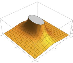
149 14.6 DIRECTIONAL DERIVATIVES AND THE GRADIENT Example. For f (x, y) = xe y y at (2, 0), what is the maximum directional derivative and what direction does it occur in? Note. Consider the graph of f on the x-y plane drawn below. Since f points in the direction of greatest increase, where do you expect the level curves to be? f (x, y) = xe y y

150 14.6 DIRECTIONAL DERIVATIVES AND THE GRADIENT Theorem. For a function f of two variables, the level curves of f are to f. Proof:

151 14.6 DIRECTIONAL DERIVATIVES AND THE GRADIENT Example. Use the gradient to find the equation of the tangent line to the level curve for f (x, y) = x 2 y 2 at (2, 3). Note. The tangent line for a level curve f (x, y) = k at the point (a, b) is given by the equation:

152 14.6 DIRECTIONAL DERIVATIVES AND THE GRADIENT Everything we have done so far can also be done for functions of three or more variables! For f (x, y, z), and unit vector u =< a, b, c > f (x 0, y 0, z 0 ) = D u f (x 0, y 0, z 0 ) = The direction of greatest increase at the point (x 0, y 0, z 0 ) is largest directional derivative has magnitude., and the f (x, y, z) is perpendicular to. The equation for a tangent plane to a level surface f (x, y, z) = k at the point (x 0, y 0, z 0 ) is given by the equation:

153 14.6 DIRECTIONAL DERIVATIVES AND THE GRADIENT Example. (# 44) Find the equation of (a) the tangent plane, and (b) the normal line to the surface xy+ yz+zx = 5 at the point (1, 2, 1). (The normal line is a line perpendicular to the surface at the given point.)

154 14.6 DIRECTIONAL DERIVATIVES AND THE GRADIENT Note. The tangent plane for the surface z = f (x, y) is the same as the tangent plane for the level surface g(x, y, z) = 0, where g(x, y, z) =. Use the equation for a tangent plane to a level surface for g(x, y, z) at (x 0, y 0, z 0 ) to find an equation for the tangent plane of z = f (x, y). Compare the equation to the equation we found in Section 14.4.

155 14.6 DIRECTIONAL DERIVATIVES AND THE GRADIENT Extra Example. Here is an example of a function that is not continuous at (0, 0) even though the directional derivatives exist in every direction! f (x, y) = xy2 x 2 + y 4

156 14.7 MAXIMUMS AND MINIMUMS 14.7 Maximums and Minimums Note. Recall: For a function f (x) of one variable, a critical point is: Note. Recall: For a function f (x) of one variable, max and min points are related to critical points. If f (x) has a local max or min at x = x 0, then x 0 (circle one) not be a critical point. If x 0 is a critical point, then f (x) (circle one) have a maximum or minimum at x 0. is / is not / may or may does / does not / may or may not

157 14.7 MAXIMUMS AND MINIMUMS Definition. For a function f (x, y) of two variables, (x 0, y 0 ) is a critical point if Theorem. If f (x, y) has a local max or local min at (x 0, y 0 ) and f x and f y exist at (x 0, y 0 ), then: 1. f x (x 0, y 0 ) = and f y (x 0, y 0 ) =. 2. D u f (x 0, y 0 ) = for all unit vectors u. 3. The tangent plane to f at (x 0, y 0 ) is Proof: Note. If (x 0, y 0 ) is a critical point, then f (circle one) does / does not / may or may not have a maximum or minimum at (x 0, y 0 ).

158 14.7 MAXIMUMS AND MINIMUMS Note. In Calc 1, we had the 2nd derivative test: If f (x 0 ) = 0 and f (x 0 ) > 0, then f has a local at x 0. If f (x 0 ) = 0 and f (x 0 ) < 0, then f has a local at x 0. Definition. The discriminant of f at (x 0, y 0 ) is given by D = Theorem. (Second Derivatives Test) Suppose that the second partial derivatives of f exist and are continuous on a disk around (x 0, y 0 ), and suppose that f x (x 0, y 0 ) = f y (x 0, y 0 ) = 0. Then (a) If D > 0 and f xx (x 0, y 0 ) > 0, then f has a at (x 0, y 0 ). (b) If D > 0 and f xx (x 0, y 0 ) < 0, then f has a at (x 0, y 0 ). (c) If D < 0 then f has a at (x 0, y 0 ). (d) If D = 0, then. (e) If D > 0 and f xx (x 0, y 0 ) = 0, then.

159 14.7 MAXIMUMS AND MINIMUMS Example. Find the local maxes and mins for. f (x, y) = x 2 + y 2 + x 2 y + 4

160 14.7 MAXIMUMS AND MINIMUMS Example. (# 40) Find the point on the plane x 2y + 3z = 6 that is closest to the point (0, 1, 1).

161 14.7 MAXIMUMS AND MINIMUMS Note. Recall, in Calc 1: If f is continuous and [a, b] is a closed interval, then f (x) (circle one) must / may or may not achieve a maximum and minimum value on [a, b]. The maximum value of f on [a, b] occurs (circle one) at one of the end points a or b / at a critical point / either at a critical point or at one of the end points a or b. Question. How do we generalize the idea of a closed interval to R 2? On which of these would you expect a continuous function to always have a max and a min? Definition. (Informal definition) A closed set is one that contains all of its boundary points. Definition. A bounded set is one that is contained inside some large disk.

162 14.7 MAXIMUMS AND MINIMUMS Theorem. (Extreme Value Theorem) If f (x, y) is continuous on a closed bounded set D, then f attains (at least one) absolute max and abs min. The absolute max and min occur either at critical points or on the boundary of D. Notation. D means the boundary of a region D. Note. To find the abs max and min of f on D

163 14.7 MAXIMUMS AND MINIMUMS Example. Find the abs max and min of f (x, y) = x 2 2xy + 2y on the triangular region with vertices (0, 2), (3, 0), (3, 2).

164 14.7 MAXIMUMS AND MINIMUMS Theorem. (Second Derivatives Test) Suppose that the second partial derivatives of f exist and are continuous on a disk around (x 0, y 0 ), and suppose that f x (x 0, y 0 ) = f y (x 0, y 0 ) = 0. Then (a) If D > 0 and f xx (x 0, y 0 ) > 0, then f has a at (x 0, y 0 ). (b) If D > 0 and f xx (x 0, y 0 ) < 0, then f has a at (x 0, y 0 ). (c) If D < 0 then f has a at (x 0, y 0 ). Proof of the Second Derivatives Test (if time)

165 14.8 LAGRANGE MULTIPLIERS 14.8 Lagrange Multipliers Example. Find the rectangle of largest area that can be inscribed in the ellipse x2 4 + y2 9 = 1 (with sides parallel to the x and y axes)

166 14.8 LAGRANGE MULTIPLIERS Consider the graph of f (x, y) = 4xy and the graph of x2 4 + y2 9 the left). = 1 in 3-dimensions (on Consider the graph of the level curves of f (x, y) = 4xy and the graph of x2 4 + y2 9 = 1 in 2-dimensions (on the right).

167 14.8 LAGRANGE MULTIPLIERS Theorem. (Lagrange multipliers) To find the max and min values of f (x, y) subject to the constraint g(x, y) = k (assuming these extreme values exist and g 0 on the constraint curve g(x, y) = k), we need to: 1. find all values (x 0, y 0 ) such that f is parallel to g, i.e. where f = λ g for some λ R. 2. compare the size of f (x 0, y 0 ) on all these candidate points. Note. In practice, we set f x (x, y) = λg x (x, y) f y (x, y) = λg y (x, y) g(x, y) = k and solve this system of equations for x, y, and λ. Note. For this to work, g must be smooth (have continuous g x and g y ) Otherwise we must also check corners and cusps where g x or g y don t exist or have discontinuities.

168 14.8 LAGRANGE MULTIPLIERS Note. Method of Lagrange multipliers also works to maximize or minimize functions f (x, y, z) of 3 variables, subject to a constraint surface g(x, y, z) = k. We set f x (x, y, z) = λg x (x, y, z) f y (x, y, z) = λg y (x, y, z) f z (x, y, z) = λg z (x, y, z) g(x, y, z) = k and solve this system of equations for x, y, z, and λ.

169 14.8 LAGRANGE MULTIPLIERS Example. Find the rectangle of largest area that can be inscribed in the ellipse x2 4 + y2 9 = 1, using Lagrange multipliers.

170 14.8 LAGRANGE MULTIPLIERS Example. Find the point on the plane x 2y + 3z = 6 that is closest to the point (0, 1, 1).

171 Example. Maximize f (x, y) = 2x 3 + y 4 on the disk D = {(x, y) x 2 + y 2 1} LAGRANGE MULTIPLIERS

172 15.1 DOUBLE INTEGRALS 15.1 Double Integrals In Calculus 1, we defined the integral of f (x) over an interval [a, b] as the limit of a Riemann sum:

173 15.1 DOUBLE INTEGRALS For a function f (x, y) over a rectangular region R = [a, b] [c, d] we can define an integral similarly: R f (x, y)da =

174 15.1 DOUBLE INTEGRALS Example. For each problem, estimate the integral of f (x, y) over the rectangle specified: 1. (# 8) The figure shows the level curves of a function f. Estimate f (x, y) da where R R = [0, 2] [0, 2]. 2. (# 14) Find R 9 y 2 da, where R = [0, 8] [0, 3]. Hint: draw a sketch. 3. (# 5) Find f (x, y) da, where R = [0, 4] [2, 4], using the midpoint rule with R n = m = 2.

175 15.2 ITERATED INTEGRALS OVER RECTANGULAR REGIONS 15.2 Iterated Integrals over Rectangular Regions To compute the double integrals of a function f (x, y) over a rectangle, it is easiest to think in terms of volume. If R = [a, b] [c, d], then Volume = b a A(x) dx, where A(x) = So f (x, y) da =. R

176 15.2 ITERATED INTEGRALS OVER RECTANGULAR REGIONS Similarly, if we look at cross-sectional area in the other direction A(y), we can compute the volume over the rectangle R = [a, b] [c, d] as: R f (x, y) da =. This is known as Fubini s Theorem. Theorem. Fubini s Theorem If f is continuous on the rectangle R = [a, b] [c, d], then the double integral equals the iterated integrals, i.e. f (x, y) da = R This theorem still holds true if we just assume that f is bounded on R, discontinuous only on a finite number of smooth curves, and the iterated integrals exist.

177 Example. (# 3) Calculate (6x 2 y 2x) da, where R R = (x, y) 1 x 4, 0 y ITERATED INTEGRALS OVER RECTANGULAR REGIONS

178 Example. (# 28) Find the volume enclosed by the surface z = 1 + e x sin y and the planes x = ±1, y = 0, y = π, and z = ITERATED INTEGRALS OVER RECTANGULAR REGIONS

179 15.3 DOUBLE INTEGRALS OVER GENERAL REGIONS 15.3 Double Integrals over General Regions Example. Calculate and y = 1 + x 2. (x 2 + 2y) da for the region D bounded by the parabolas y = 2x 2 D

180 15.3 DOUBLE INTEGRALS OVER GENERAL REGIONS Example. Calculate y 2 = 2x + 6. D y da for the region D bounded by the parabolas y = x 1 and

181 15.3 DOUBLE INTEGRALS OVER GENERAL REGIONS These two regions are examples of Type I and Type II regions. Type I Region For a Type I region, For a Type II region, D D f (x, y) da = f (x, y) da = Type II Region Note. If a region is both a Type I region and a Type II region, sometimes, it is easier to evaluate the integral in one way instead of the other.

182 15.3 DOUBLE INTEGRALS OVER GENERAL REGIONS Example. (# 54) Evaluate 8 2 e x4 0 3 y dx dy

183 15.3 DOUBLE INTEGRALS OVER GENERAL REGIONS Example. Find an upper and lower bound for where D is the disk {(x, y) x 2 + y } D e (x2 +y 2) dx dy

184 15.3 DOUBLE INTEGRALS OVER GENERAL REGIONS Left-over from Section 15.2: Question. True or False: 6 1 f (x)g(x) dx = 6 1 f (x) dx 6 1 g(x) dx Question. True or False: f (x)g(y) dx dy = 9 5 f (x) dx 6 1 g(y) dy Question. True or False: 6 y f (x)g(y) dx dy = y 2 5 f (x) dx 6 1 g(y) dy

185 15.4 INTEGRATION USING POLAR COORDINATES 15.4 Integration using Polar Coordinates Note. Recall: The polar coordinates of a point in the plane are given by (r, θ), where r is the distance from the origin (radius) and θ is the angle made with the positive x-axis. Note. A negative angle means to go clockwise from the positive x-axis. A negative radius means jump to the other side of the origin, that is, ( r, θ) means the same point as (r, θ + π)

186 15.4 INTEGRATION USING POLAR COORDINATES Note. Recall: To convert between polar and Cartesian coordinates, note that: x = y = r 2 = tan(θ) =

187 15.4 INTEGRATION USING POLAR COORDINATES Example. (# 5 and # 6) Sketch the region described. 1. {(r, θ) π 4 θ 3π 4, 1 r 2} This is an example of a polar rectangle. 2. {(r, θ) π 2 θ π, 0 r 2 sin θ}

188 Example. (# 7) Evaluate origin and radius 5. D 15.4 INTEGRATION USING POLAR COORDINATES x 2 y da, where D is the top half of the disk with center the

189 15.4 INTEGRATION USING POLAR COORDINATES Theorem. If f (x, y) is continuous on a polar rectangle R = {(r, θ) α θ β, a r b}, then R f (x, y) da = Proof. (Where does the extra r come from?)

190 15.4 INTEGRATION USING POLAR COORDINATES Example. (# 21) Find the volume enclosed by the hyperboloid x 2 y 2 + z 2 = 1 and the plane z = 2.

191 15.4 INTEGRATION USING POLAR COORDINATES Integration over more general regions: Theorem. If f (x, y) is continuous on the region R = {(r, θ) α θ β, h 1 (θ) r h 2 (θ)}, then R f (x, y) da =

192 15.4 INTEGRATION USING POLAR COORDINATES 3 Example. (# 16) Find the area of the region enclosed by both of the cardioids r = 1+cos θ and r = 1 cos θ

193 15.4 INTEGRATION USING POLAR COORDINATES Example. The equation of the standard normal curve (with mean 0 and standard deviation 1) is f (x) = 1 2π e x2 2 Prove that the area under the standard normal curve is 1.

194 15.5 CENTER OF MASS 15.5 Center of Mass Example. Suppose we have 4 children Abe, Beatrice, Catalonia, and Drew sitting on a see-saw. The children have masses 25 kg, 30 kg, 10 kg, and 35 kg, respectively, and are at distances 1 ft, 3 ft, 5 ft, and 7 ft from the left end of the see-saw. To balance the seesaw perfectly, where should the fulcrum be? (Ignore the mass of the seesaw itself.)

195 15.5 CENTER OF MASS Now suppose we have a thin rod lying along the x-axis between x = a and x = b. The rod is made of a non-uniform material whose density at position x is given by a function ρ(x). If we want to balance the rod, where should we place the fulcrum?

196 15.5 CENTER OF MASS Now suppose we have a lamina (thin sheet) in the shape of a region D. The density of the lamina at point (x, y) is given by the function ρ(x, y). If we want to balance the lamina, where should we place the fulcrum? Definition. The balance point (x, y) is called the. The numerator of the expression for x is called the moment about the and is written as. The numerator of the expression for y is called the moment about the and is written as. The denominator of the expressions for x and y is the.

197 15.5 CENTER OF MASS Example. SET UP the equations to find the mass and the center of mass of a region enclosed by the curves x = y 2 and x = 4, if ρ(x, y) = x + y 2.

198 15.5 CENTER OF MASS Example. A lamina occupies the part of the first quadrant that is inside a disk of radius 5 and outside a disk of radius 1. Find its center of mass if the density at any point is inversely proportional to its distance from the origin.

199 15.6 SURFACE AREA 15.6 Surface Area To find the surface afea of a surface z = f (x, y), we approximate the surface with little pieces of planes that lie above little rectangles on the x-y plane. What is the area of a parallelogram formed by two vectors? What are the vectors that run along the sides of the little pieces of planes?

200 15.6 SURFACE AREA What is the area of a little piece of plane in the figure? What is the area of the surface z = f (x, y), for (x, y) in some region D?

201 15.6 SURFACE AREA Example. (#12) Find the surface area of the part of the sphere x 2 + y 2 + z 2 = 4z that lies inside the paraboloid z = x 2 + y 2.

202 15.7 TRIPLE INTEGRALS 15.7 Triple Integrals The integral of f (x, y, z) over a rectangular box B = [a, b] [c, d] [r, s] can be defined as a limit of a Riemann sum: B f (x, y, z) dv = Theorem. (Fubini s Theorem for Triple Integrals) If f (x, y, z) is continuous over the box B, then B f (x, y, z) dv =

203 15.7 TRIPLE INTEGRALS Integrals over general regions. Example. (# 10) Evaluate the triple integral: E e z/y dv where E = {(x,, y, z) 0 y 1, y x 1, 0 z xy}

204 Example. (# 18) Set up the bounds of integration for E 15.7 TRIPLE INTEGRALS f (x, y, z)dv, where E is bounded by the cylinder y 2 + z 2 = 9 and the planes x = 0, y = 3x, and z = 0 in the first octant.

205 15.7 TRIPLE INTEGRALS Extra Example. (# 34) Rewrite the integral by changing the order of integration in as many ways as possible. 1 1 x 2 1 x f (x, y, z) dy dz dx

206 15.7 TRIPLE INTEGRALS Example. Suppose I wanted to find the volume of this solid. Could I compute it using a double integral? Could I compute it using a triple integral?

207 15.8 TRIPLE INTEGRALS IN CYLINDRICAL COORDINATES 15.8 Triple Integrals in Cylindrical Coordinates Note. The cylindrical coordinates of a point in the plane are given by (r, θ, z), where z is the height and r and θ are the polar coordinates of the projection of the point onto the x-y plane. As with polar coordinates, r can be positive or negative. Note. Cartesian coordinates and cylindrical coordinates are related by: x = y = z = r 2 = tan θ =

208 15.8 TRIPLE INTEGRALS IN CYLINDRICAL COORDINATES Example. What surfaces are described by these equations? 1. r = 5 2. θ = π 3 3. z = r 4. z 2 = 4 r 2

209 15.8 TRIPLE INTEGRALS IN CYLINDRICAL COORDINATES Note. Using cylindrical coordinates, if E is a region of space that can be described by: α θ β, h 1 (θ) r h 2 (θ), u 1 (r, θ) z u 2 (r, θ), then E f (x, y, z) dv =

210 15.8 TRIPLE INTEGRALS IN CYLINDRICAL COORDINATES Example. Find the mass of the solid cone bounded by z = 2r and z = 6, if the density at any point is proportional to its distance from the z-axis.

211 15.8 TRIPLE INTEGRALS IN CYLINDRICAL COORDINATES Example. (#30) Rewrite the integral in cylindrical coordinates. 3 9 x 2 9 x 2 y x 2 + y 2 dz dy dx Hint: project the region onto the x-y plane and write this in polar coordinates.

212 15.8 TRIPLE INTEGRALS IN CYLINDRICAL COORDINATES Extra Example. (#31) Consider a mountain that is in the shape of a right circular cone. Suppose that the weight density of the material in the vicinity of a point P is g(p) and the height is h(p). 1. Find a definite integral that represents the total work done in forming the mountain. 2. Assume that Mount Fiji is in the shape of a right circular cone with radius 19,000 meters, height 3,800 meters, and density a constant 3,200 kg/m 3. How much work was done in forming Mount Fiji if the land was initially at sea level?

213 15.9 TRIPLE INTEGRALS IN SPHERICAL COORDINATES 15.9 Triple Integrals in Spherical Coordinates Note. The spherical coordinates of a point in the plane are given by (ρ, θ, φ), where ρ is the distance from the origin, θ is the angle with the positive x-axis, and φ is the angle with the positive z-axis. Note. For spherical coordinates, ρ 0 always. Also, 0 φ π always. Note. Cartesian coordinates and spherical coordinates are related by: x = y = z = ρ = tan θ = tan φ =

214 15.9 TRIPLE INTEGRALS IN SPHERICAL COORDINATES Example. What surfaces are described by these equations? 1. ρ = 5 2. θ = π 4 3. φ = π 6.

215 15.9 TRIPLE INTEGRALS IN SPHERICAL COORDINATES Note. Using spherical coordinates, for a ρ b, α θ β, γ φ δ, Proof. (Informal Justification) E f (x, y, z) dv =

216 15.9 TRIPLE INTEGRALS IN SPHERICAL COORDINATES Example. (# 30) Find the volume of the solid that lies within the sphere x 2 + y 2 + z 2 = 4, above the x-y plane, and below the cone z = x 2 + y 2.

217 15.9 TRIPLE INTEGRALS IN SPHERICAL COORDINATES Example. (# 41) Change the integral to spherical coordinates. 2 4 x x 2 y x 2 (x 2 4 x 2 + y 2 + z 2 ) 3/2 dz dy dx 2 y 2

218 15.9 TRIPLE INTEGRALS IN SPHERICAL COORDINATES Extra Example. (#28) Find the average distance from a point in a ball of radius a to its center.

219 15.10 CHANGE OF VARIABLES Change of Variables In Calc 1, we use u-substitution to do a change of variables. Example. π 0 sin(x 2 )2x dx = General formula for change of variables in 1-dimension: b a f (g(x))g (x) dx = To agree with the notation in the book, reverse the roles of x and u to get: b a f (g(u))g (u) du = Goal: generalize this change of variables formula to 2 and 3 dimensions. First, need to define what we mean by a change of variables.

220 15.10 CHANGE OF VARIABLES Definition. A C 1 transformation is a function ( mapping ) by T : R R R R T(u, v) = (g(u, v), h(u, v)) for functions g and h with continuous first derivatives. Definition. A transformation T is one to one if... Example. T(r, θ) = (r cos θ, r sin θ) g(r, θ) = h(r, θ) = T : [0, 1] [0, π]

221 15.10 CHANGE OF VARIABLES Example. T(u, v) = ( ) v u, u2 v x(u, v) =, y(u, v) = Where does T map the unit square S = {(u, v) 1 u 2, 1 v 2}?

222 15.10 CHANGE OF VARIABLES Definition. The Jacobian J of a transformation T is given by T(u, v) = (x(u, v), y(u, v)) is (x, y) (u, v) = x u y u x v y v = x y u v y u x v Example. Compute the Jacobian for the transformation x = v u, y = u2 v.

223 15.10 CHANGE OF VARIABLES Theorem. Suppose T is a C 1 transformation whose Jacobian is non-zero and maps a region S in the u-v plane to a region R in the x-y plane. Suppose that T is one-to-one, except possibly on the boundary. Then for a continuous function f, S f (x(u, v), y(u, v)) abs ( x u y u x v y v ) du dv = R f (x, y) dx dy

224 15.10 CHANGE OF VARIABLES For transformations in 3-dimensions: Definition. For T : R R R R R R the Jacobian J is given by T(u, v, w) = (x(u, v, w), y(u, v, w), z(u, v, w)) (x, y, z) (u, v, w) = and the conclusion of the theorem is that: x u x v x w y u y v y w z u z v z w S f (x(u, v, w), y(u, v, w), z(u, v, w)) abs x u y u z u x v y v z v x w y w z w du dv dw = R f (x, y, z) dx dy dz

225 15.10 CHANGE OF VARIABLES Example. (Like #20) Use a change of variables to evaluate R x 2 da where R is the region bounded by the curves xy = 1, xy = 2, x 2 y = 1, and x 2 y = 2.

226 15.10 CHANGE OF VARIABLES Example. (# 25) Make a change of variables to evaluate the integral R ( ) y x cos da y + x where R is the trapezoidal region with vertices (1, 0), (2, 0), (0, 2), and (0, 1).

227 15.10 CHANGE OF VARIABLES Theorem. (Change to polar coordinates) If f (x, y) is continuous on some region R given by R = {(r, θ) a r b, α θ β}, where a, b > 0 and 0 β α 2π, then R f (x, y) da = β b α a f (r cos θ, r sin θ) r dr dθ

228 15.10 CHANGE OF VARIABLES Theorem. (Change to spherical coordinates) If f (x, y, z) is continuous on some region R given by R = {(ρ, θ, φ) a ρ b, α θ β, γ φ δ}, then R f (x, y, z) da = δ β b γ α a f (ρ sin φ cos θ, ρ sin φ sin θ, ρ cos φ) ρ 2 sin φ dρ dθdφ

229 Note. Explanation for why the Jacobian is the right thing to multiply by: CHANGE OF VARIABLES

230 16.1 VECTOR FIELDS 16.1 Vector Fields Definition. A vector field on R 2 is a function F(x, y) : D R 2 R 2 where D is a subset of R 2. We usually think of the output as a two-dimensional vector.

231 16.1 VECTOR FIELDS Definition. A vector field on R 3 is a function F(x, y, z) : E R 3 R 3. where E is a subset of R 3 We usually think of the output as a three-dimensional vector. Example. The gradient f of a function or two or three variables is a vector field.

232 16.1 VECTOR FIELDS Example. Match the vector field with the plot. A) B) C) D) 1) F(x, y) = cos(x + y) i + x j 2) G(x, y) = i + x j 3) H(x, y) = y i + (x y) j 4) J(x, y) = y x2 + y 2 i + x x2 + y 2 j

233 16.1 VECTOR FIELDS Example. The force of gravity can be written as a vector field. Let M = mass of earth m = mass of object G = gravitational constant F = force of gravity Newton s law says F = mmg, where r is the diestance between the object and the center of the earth. r 2 Write F as a vector field. Hint: put the origin at the center of the earth.

234 16.1 VECTOR FIELDS Definition. A vector field F is conservative if it is the gradient of some function. That is, there exists a function f such that F = f. Definition. If F = f, then f is called the for F. Question. Is the force of gravity a conservative vector field? Question. Are their vector fields that aren t conservative? Give an example.

235 16.2 LINE INTEGRALS 16.2 Line Integrals Final Goal: define an integral of a vector field over a curve important applications to fluid flows, electricity and magnetism, etc. First step: define the integral of a function over a curve, for a function with input in R 2 or R 3 and output in R. note: old definition of f da cannot be used for an integral over a curve, why? R start with functions of 2-dimensions and then extend the ideas and formulas to 3-dimensions. We start with a curve C parametrized by r(t) =< x(t), y(t) > for a t b In this section, we will work only with curves that are piecewise smooth, which means that the curve can be divided into finitely many pieces, and each for each piece:

236 16.2 LINE INTEGRALS We want to define f (x, y) ds, the integral of a function of 2 variables over a curve C with respect to arclength. Think of the function as the height of a vertical curtain over the curve, and think of the integral as the area of this curtain. Special case: If f (x, y) = 1, then C f (x, y) ds should equal... Definition. The line integral of f over C with respect to arc length is given by: C f (x, y) ds =

237 16.2 LINE INTEGRALS Note. It is also possible to define C equivalent. f (x, y) ds as the limit of a Riemann sum, which is Note. The line integral of f over C with respect to arc length does not depend on the parametrization of C as long as the parametrization goes from t = a to t = b with a < b.

238 16.2 LINE INTEGRALS Example. (# 2) Calculate C xy ds, for C : x = t 2, y = 2t, 0 t 1.

239 16.2 LINE INTEGRALS Some other kinds of line integrals: Definition. The line integral of f with respect to x is C f (x, y) dx = The line integral of f with respect to y is C f (x, y) dy = The line integral C f (x, y) dx + g(x, y) dy = Note. The line integral with respect to x and the line integral with respect to y are independent of parametrization provided that the parametrizations traverse C in the same direction.

240 Example. (#8) Find C 16.2 LINE INTEGRALS x 2 dx + y 2 dy where C consists of the arc of the circle x 2 + y 2 = 4 from (2, 0) to (0, 2) followed by the line segment from (0, 2) to (4, 3).

241 16.2 LINE INTEGRALS Finally, the last kind of line integrals: the line integral of a vector field over a curve. We want to define F dsomething, and get a scalar answer. C Definition. For a vector field F(x, y) over a curve C parametrized by r(t) =< x(t), y(t) >, define the line integral of F over C by: F d r = C Equivalently, this can be written in terms of the components of r(t). Equivalently, this can be written in terms of a line integral of a function with respect to arc length (hint: first write it in terms of the unit tangent vector):

242 16.2 LINE INTEGRALS Equivalently, this can be written in terms of a line integrals of a function with respect to x and with respect to y. First, write F in components as F(x, y) =< P(x, y), Q(x, y) >. Then:

243 16.2 LINE INTEGRALS Motivation for this definition comes from the physics concept of work. Work = force distance Find an expression for the work done by a vector field F(x, y) as it pushes a particle along a curve C.

244 16.2 LINE INTEGRALS Example. (# 39) Find the work done by the force field F(x, y) = x i + (y + 2) j in moving an object along an arch of the cycloid r(t) = (t sin t) i + (1 cos t) j for 0 t 2π.

245 16.2 LINE INTEGRALS There are analogous definitions for functions and vector fields of 3-variables: For a function f (x, y, z), and a curve C in R 3 parametrized by r(t) =< x(t), y(t), z(t) >, Definition. C f (x, y, z) ds = The line integral of f (x, y, z) with respect to x is C f (x, y, z) dx = The line integral of f (x, y, z) with respect to y is C f (x, y, z) dy = The line integral of f (x, y, z) with respect to z is C The line integral C f (x, y, z) dz = f (x, y, z) dx + g(x, y, z) dy + h(x, y, z) dz =

246 16.2 LINE INTEGRALS For a vector function F(x, y, z) in R 3 F(x, y, z) d r = C

247 16.2 LINE INTEGRALS Note. All of these line integrals are independent of the parametrization of C up to a positive or negative sign. There are some subtleties as far as which parametrizations give the exact same value and which parametrizations give opposite values. Example. Let f (x, y) = 3. For the following five curves, sketch the curve and calculate C f (x, y) ds 1. C 1 : r 1 (t) =< cos t, sin t >, 0 t π 2 2. C 2 : r 2 (t) =< cos t, sin t >, t runs from π 2 to C 3 : r 3 (t) =< sin t, cos t >, 0 t π 2 4. C 4 : r 4 (t) =< sin t, cos t >, t runs from π 2 to C 5 : r 5 (t) =< cos 2t, sin 2t >, 0 t π 4 Conclusion: C f (x, y) ds does not depend on parametrization, as long as...

248 16.2 LINE INTEGRALS Example. Let f (x, y) = 3. For the following five curves, sketch the curve and calculate C f (x, y) dx 1. C 1 : r 1 (t) =< cos t, sin t >, 0 t π 2 2. C 2 : r 2 (t) =< cos t, sin t >, t runs from π 2 to C 3 : r 3 (t) =< sin t, cos t >, 0 t π 2 4. C 4 : r 4 (t) =< sin t, cos t >, t runs from π 2 to C 5 : r 5 (t) =< cos 2t, sin 2t >, 0 t π 4 Conclusion: C f (x, y) dx does not depend on parametrization, as long as...

249 16.2 LINE INTEGRALS Question. What can we say about C F(x, y) d r and the effect of parametrization?

250 16.3 FUNDAMENTAL THEOREM FOR LINE INTEGRALS 16.3 Fundamental Theorem for Line Integrals We will state and prove results for vector fields in R 2, but they also hold for vector fields in R 3. We will only work with piecewise smooth curves. Recall: in Calc 1, the Fundamental Theorem of Calculus (FTC) says: b a F (x) dx = For line integrals, we have a similar theorem where F. plays the role of

251 16.3 FUNDAMENTAL THEOREM FOR LINE INTEGRALS Theorem. (Fundamental Theorem for Line Integrals - FTLI) Let f (x, y) be a differentiable function whose gradient is continuous. Let C be a smooth curve parametrized by r(t) for a t b. Then C f d r = Proof. Use the chain rule in reverse:

252 16.3 FUNDAMENTAL THEOREM FOR LINE INTEGRALS Example. (#1) The figure shows a curve C and a contour map of a function f (x, y) = y sin(x + y) + x whose gradient f is continuous. Find C f d r

253 16.3 FUNDAMENTAL THEOREM FOR LINE INTEGRALS Example. Find the work done by gravity to move an object of mass 100 kg from the point (3.1, 3, 5) (in millions of meters) to the point (3, 3, 5). Note: the force of gravity is given by mmgx F(x, y, z) = (x 2 + y 2 + z 2 ) 3/2 i mmgy (x 2 + y 2 + z 2 ) 3/2 j mmgz (x 2 + y 2 + z 2 ) 3/2 k Recall: F = f, where f = M = kg, G = m3 kg s 2

254 16.3 FUNDAMENTAL THEOREM FOR LINE INTEGRALS Note. 1. The Fundamental Theorem of Line Integrals (FTLI) only applies to vector fields that are gradients, i.e. to conservative vector fields. 2. The FTLI says that we can evaluate the line integral of a conservative vector field f if we only know the value of f at. 3. In the language of physics, the FTLI says that the work done in moving an object from one point to another by a conservative force (like gravity) does not depend on, only on. 4. If C 1 and C 2 are two paths connecting points A and B, then C 1 f d r C 2 f d r =

255 16.3 FUNDAMENTAL THEOREM FOR LINE INTEGRALS Definition. For continuous vector field F(x, y), we say that F(x, y) d r is independent of path if C for any two curves C 1 and C 2 with the same initial and terminal end points. Question. Are there any vector fields that have line integrals that are NOT independent of path? True or False: If a vector field is conservative, then it has line integrals that are independent of path. True or False: If a vector field has line integrals that are independent of path, then it is conservative.

256 16.3 FUNDAMENTAL THEOREM FOR LINE INTEGRALS Need a few definitions to make this and subsequent facts precise. Definition. A curve C is closed if the initial point and terminal point of C coincide. Definition. A curve C is simple if C does not intersect itself, except possibly at its endpoints.

257 16.3 FUNDAMENTAL THEOREM FOR LINE INTEGRALS Definition. (Informal definition) A region D is open if it doesn t contain any of its boundary points.

258 16.3 FUNDAMENTAL THEOREM FOR LINE INTEGRALS Definition. A region D is connected if any two points in D can be joined by a path in D. Definition. A region D is simply connected if it is connected and for every simple closed curve C in D, C encloses only points of D. Infomally, simply connected means connected with no holes.

259 16.3 FUNDAMENTAL THEOREM FOR LINE INTEGRALS Classify each curve: is it simple? closed? Classify each region: is it open? connected? simply connected?

260 16.3 FUNDAMENTAL THEOREM FOR LINE INTEGRALS Theorem. Suppose F is a continuous vector field on an open, connected region D. Then F d r is independent of path C

261 16.3 FUNDAMENTAL THEOREM FOR LINE INTEGRALS Another characterization of independence of path: Theorem. Suppose F is a continuous vector field on a region D, then independent of path C F d r is for every closed path Ĉ in D. Proof:

262 16.3 FUNDAMENTAL THEOREM FOR LINE INTEGRALS Theorem. For a continuous vector field F on an open, connected region D, the following are equivalent: Note. So far all of this is true for vector fields in R 3 as well.

263 16.3 FUNDAMENTAL THEOREM FOR LINE INTEGRALS Goal: find a more practical condition to decide when a vector field is the gradient of a function and when it could not be the gradient of a function. Theorem. If F(x, y) = P(x, y) i + Q(x, y) j is f for some function f, where P(x, y) and Q(x, y) have continuous first partial derivatives, then

264 16.3 FUNDAMENTAL THEOREM FOR LINE INTEGRALS Theorem. If P y Q x on a region D, then Question. Does the converse hold? Is it true that if P y = Q x on a region D, then F = f for some function f? Theorem. If F(x, y) = P(x, y) i + Q(x, y) j is a vector field on an open, simply connected region D, and P and Q have continuous first partial derivatives, then

265 16.3 FUNDAMENTAL THEOREM FOR LINE INTEGRALS Example. Determine if F = (3 + 2xy) i + (x 2 3y 2 ) j is conservative. If it is conservative, find f such that f = F.

266 16.3 FUNDAMENTAL THEOREM FOR LINE INTEGRALS We don t yet have an analogous, easy method to determine whether a vector field in R 3 is conservative. (Wait till section 16.5). But if we know that F is conservative, then the method for finding f with f = F is the same. Example. (#18) F(x, y, z) = sin y i + (x cos y + cos z) j y sin z k is conservative. Find f such that f = F.

267 16.3 FUNDAMENTAL THEOREM FOR LINE INTEGRALS Note. If the region D is not simply connected, then P y = Q x on D does not guarantee that F is conservative. Example. Is this vector field conservative? Why or why not? F(x, y) = y x 2 + y 2 i + x x 2 + y 2 j

268 16.4 GREEN S THEOREM 16.4 Green s Theorem Green s Theorem relates a line integral over simple closed curve C to a double integral over the region that C encloses. Definition. A simple closed curve C that forms the boundary of a region D is called positively oriented if, as you traverse C, the region D is always to the left. A collection of curves C 1 C 2 C n that together form the boundary of a region D are positively oriented if each curve is positively oriented.

269 16.4 GREEN S THEOREM Theorem. Green s Theorem Let F(x, y) = P(x, y) i + Q(x, y) j be a vector field and suppose that P and Q have continuous first partial derivatives. Let D be a positively oriented, piecewise smooth curve or collection of curves that bound a region D. Then D = D Note. Alternative notations for P dx + Q dy are: P dx + Q dy OR P dx + Q dy, D C C where C = D.

270 16.4 GREEN S THEOREM Note.. 1. Green s theorem works for any vector field F (unlike the Fundamental Theorem of Line Integrals which only applies to conservative vector fields). 2. Green s theorem is analogous to the fundamental theorem of calculus: both relate the integral of a derivative of a function to a function on the boundary of the region. 3. Green s theorem applies only to 2-dimensional vector fields (but there is a more general theory that applies in n dimensions). 4. Green s theorem can be used to prove that when P y = Q x on an open, simply connected region, then F = P i + Q j is conservative.

271 16.4 GREEN S THEOREM Example. (# 9) Use Green s Theorem to evaluate the line integral along the positively oriented circle x 2 + y 2 = 4. C y 3 dx x 3 dy

272 16.4 GREEN S THEOREM Green s theorem can be used to to convert an integral over a region to a line integral. This is useful when computing area: Since that D 1 da = area(d), to use Green s Theorem, we need to find P and Q such What can we use for P and Q? Q x P y = 1 Note. area(d) = D

273 16.4 GREEN S THEOREM Extra Example. (# 21) (a) If C is the line segment connecting the point (x 1, y 1 ) to (x 2, y 2 ), show that C x dy y dx = x 1 y 2 x 2 y 1. (b) Find the area of a pentagon with vertices (0, 0), (2, 1), (1, 3). (0, 2), ( 1, 1).

274 16.4 GREEN S THEOREM Extra Example. (Example 5 from book) If F(x, y) =< y x x 2 + y 2, >, show that x 2 + y2 F d r = 2π for every positively oriented simple closed curve that encloses the origin. C

275 16.4 GREEN S THEOREM PROOFS Theorem. Green s Theorem Let F(x, y) = P(x, y) i + Q(x, y) j be a vector field and suppose that P and Q have continuous first partial derivatives. Let D be a positively oriented, piecewise smooth curve or collection of curves that bound a region D. Then ( Q P dx + Q dy = x P ) da y Proof.. Step 1: Prove that if D is a Type I region, then Step 2: Prove that if D is a Type II region, then D D D D ( P dx = P ) da. D y ( ) Q Q dy = da. y Step 3: Prove Green s Theorem for regions that are both Type I and Type II. Step 4: Prove Green s Theorem in general. D

276 16.5 DIVERGENCE AND CURL 16.5 Divergence and Curl Note. Divergence (div) and curl apply to vectors in 3-dimensions. Definition. (Informal definition) If F represents the velocity of a fluid, then div F(x, y, z) represents the net flow from the point (x, y, z). F =< x, y, 0 > F =< 2y, 2x, 0 > F =< y 3 + 1, 0, 0 > F =< x + 2, y + 2, 0 > Example. (#9-11) The vector field F = P i + Q j + R k is shown in the xy plane and looks the same in all other horizontal planes. Is div F positive, negative, or zero at the origin?

277 16.5 DIVERGENCE AND CURL Definition. For F = P i + Q j + R k, the divergence div F is defined as: Note that div F is a (circle one) scalar / vector.

278 16.5 DIVERGENCE AND CURL Definition. (Informal definition) If F represents the velocity of a fluid, then curl F(x, y, z) represents the net rotation of the fluid around the point (x, y, z). The direction of the curl is the axis of rotation, as determined by the right-hand rule, and the magnitude of the curl is the magnitude of rotation. F(x, y, z) =< x, y, 0 > F(x, y, z) =< 2y, 2x, 0 > F(x, y, z) =< y 3 + 1, 0, 0 > F(x, y, z) =< x + 2, y Example. (#9-11) The vector field F = P i + Q j + R k is shown in the xy plane and looks the same in all other horizontal planes. Determine whether curl F = 0 at the origin. If not, in which direction does curl F point?

279 16.5 DIVERGENCE AND CURL Definition. For F = P i + Q j + R k, the curl F is defined as: Note that curl F is a (circle one) scalar / vector.

280 16.5 DIVERGENCE AND CURL Example. Compute the divergence and curl of the previous 4 examples: 1. F(x, y, z) =< x, y, 0 > 2. F(x, y, z) =< 2y, 2x, 0 > 3. F(x, y, z) =< y 3 + 1, 0, 0 > 4. F(x, y, z) =< x + 2, y + 2, 0 >

281 16.5 DIVERGENCE AND CURL Example. (# 4) For the vector field F(x, y, z) = sin yz i + sin zx j + sin xy k. 1. Find div( F) 2. Find curl( F) 3. Find div(curl( F))

282 16.5 DIVERGENCE AND CURL Theorem. If F = P i + Q j + R k is a vector field on R 3 and P, Q, and R have continuous second-order partial derivatives, then Proof: div curl F =

283 16.5 DIVERGENCE AND CURL Theorem. For any function f on R 3 with continuous second-order derivatives, curl( f ) =. Proof: Question. Is F(x, y, z) = sin yz i + sin zx j + sin xy k conservative?

284 16.5 DIVERGENCE AND CURL We have that if F is conservative, then curl F = 0. What about the converse? Theorem. If F is a vector field defined on a simply connected open region of R 3. Assume all the component functions of F have continuous partial derivatives and suppose that curl F = 0. Then... Proof is a consequence of Stoke s Thm in Section 16.8.

285 16.5 DIVERGENCE AND CURL Review. In 3-dimensions, we have F = f curl F = 0 In 2-dimensions, we saw F = f Q y P x = 0 The 2-d fact is a special case of the 3-d fact:

286 16.5 DIVERGENCE AND CURL Vector forms of Green s Theorem Green s Theorem (which relates to 2-dim vector fields) can also be stated in terms of curl and divergence for associated 3-dim vector fields.

287 16.6 PARAMETRIC SURFACES 16.6 Parametric Surfaces Review. A parametric curve r(t) =< x(t), y(t), z(t) > gives the x, y, and z coordinates of points on the curve in terms of a third variable t. Definition. A parametric surface r(u, v) =< x(u, v), y(u, v), z(u, v) > gives the x, y, and z coordinates of points on the surface in terms of two parameters u and v. Example. Graph the parametric surface for 0 u 2π, 0 v 2π. r(u, v) =< cos(u), sin(u) + cos(v), sin(v) >

288 16.6 PARAMETRIC SURFACES Example. (# 19) Parametrize the plane through the point (0, 1, 5) that contains the vectors < 2, 1, 4 > and < 3, 2, 5 >.

289 16.6 PARAMETRIC SURFACES Example. (#22) Parametrize the part of the ellipsoid x 2 + 2y 2 + 3z 2 = 1 that lies in the half-space where y 0.

290 16.6 PARAMETRIC SURFACES Tangent Planes: Find the tangent plane to the surface r(u, v) =< cos(u), sin(u) + cos(v), sin(v) > at the point (1, 1, 0)

291 16.6 PARAMETRIC SURFACES Goal: Find the surface area of a parametric surface r(u, v) =< x(u, v), y(u, v), z(u, v) >

292 16.6 PARAMETRIC SURFACES Example. (# 48) Find the surface area of the helicoid (spiral ramp) x = u cos(v), y = u sin(v), z = v. for 0 < u < 5, 0 < v < 4π.

293 16.6 PARAMETRIC SURFACES Note. There are alternative formulas for surface area in special cases. 1. If the surface is of the form z = f (x, y), then surface area is given by: 2. If the surface is a surface of revolution, formed by rotating the curve y = g(x) around the x-axis for a x b, then surface area is given by: Both of these formulas can be derived from the general formula for the area of a parametric surface.

294 16.7 SURFACE INTEGRALS 16.7 Surface Integrals Preliminaries: Definition. An orientation of a surface S in R 3 is a choice of unit normal vector n(x, y, z) at every point (x, y, z) S, in such a way that n varies continuously. Example. A hemisphere has two orientations: Definition. A surface is orientable if it is possible to find an orientation for it. Question. Are all surfaces orientable?

295 16.7 SURFACE INTEGRALS Note. A surface in R 3 is orientable if and only if it has two sides. Any orientable surface has two orientations. Definition. For a closed surface in R 3 (finite with no boundary), the positive orientation is the orientation for which the normal vectors point. The negative orientation is the orientation for which the normal vectors point.

296 16.7 SURFACE INTEGRALS A surface integral is analogous to a line integral. Review. The line integral of f (x, y) with respect to arclength over the curve C is defined as: C f (x, y, z)ds = and represents:

297 16.7 SURFACE INTEGRALS Definition. The surface integral of f (x, y, z) over the parametrized surface S is defined as: S f (x, y, z)ds = and represents: If the surface is described as z = g(x, y) for some function g, then S f (x, y, z)ds =

298 16.7 SURFACE INTEGRALS Review. The line integral of a vector field F(x, y, z) is defined as F d r = C and represents:

299 16.7 SURFACE INTEGRALS Definition. The surface integral of a function F(x, y, z) over a parametrized surface S is: S F(x, y, z) d S = This represents: Note. The surface integral of F(x, y, z) over the surface S can be calculated as: F(x, y, z) ds = S

300 16.7 SURFACE INTEGRALS Why does S F n ds represent flux (rate of fluid flow)?

301 16.7 SURFACE INTEGRALS If the surface is described as z = g(x, y) and F = P i + Q j + R k for (x, y) D, then Proof: S F(x, y, z) d S = D P g x Q g y + R da

302 16.7 SURFACE INTEGRALS Question. Are surface integrals well-defined? If we use two different parametrizations of a surface, will we still get the same answer for the surface integral?

303 16.7 SURFACE INTEGRALS Example. (# 46) Gauss s Law says that the net charge enclosed by a closed surface S is where ɛ 0 is a constant. q = ɛ 0 S E d S Use Gauss s Law to find the charge enclosed by the cube with vertices (±1, ±1, ±1) if the electric field is E(x, y, z) = x i + y j + z k.

304 16.7 SURFACE INTEGRALS Extra Example. (# 47) The temperature at the point (x, y, z) in a substance with conductivity K = 6.5 is u(x, y, z) = 2y 2 + 2z 2. The heat flow is defined as F = K u Find the rate of heat flow inward across the cylindrical surface y 2 + z 2 = 6, 0 x 4.

305 16.7 SURFACE INTEGRALS Extra Example. (#44) Seawater has density 1025 kg/m 3 and flows in a velocity field v = y i + x j, where x, y, and z are in meters and the components of v are in m/sec. Find the rate of flow outward through the hemisphere x 2 + y 2 + z 2 = 9, z 0.

306 16.7 SURFACE INTEGRALS Extra Example. (# 7) Set up the equation to find y ds, where S is the helicoid with S vector equation r(u, v) =< u cos(v), u sin(v), v > with 0 u 1, 0 v π.

307 16.7 SURFACE INTEGRALS Extra Example. (#22) Set up the equation to find S F ds, where F(x, y, z) = z i+ y j+x k and S is the helicoid again: r(u, v) =< u cos(v), u sin(v), v > with 0 u 1, 0 v π.

308 16.8 STOKES THEOREM 16.8 Stokes Theorem Preliminaries: If S is an oriented surface with boundary S, a positive orientation on S means that if you walk around S with your head in the direction of the normal vector for S, the surface S lies on your left. Review. Green s Theorem says that for F =< P, Q > (assuming P, Q have continuous partials and D is piecewise smooth). D P dx + Q dy = D Q x P y da This can also be written as F d r =. D D curl( F) k da

309 16.8 STOKES THEOREM Theorem. (Stoke s Theorem) Let S be an oriented piecewise smooth surface bounded by a simple, closed, piecewise smooth boundary curve S with positive orientation. Let (F) be a vector field whose components have continuous partial derivatives in an open region of R 3 around S. Then This can also be written as In words this means: S S F d r = F d r = S S curl( F) n ds curl( F) d S

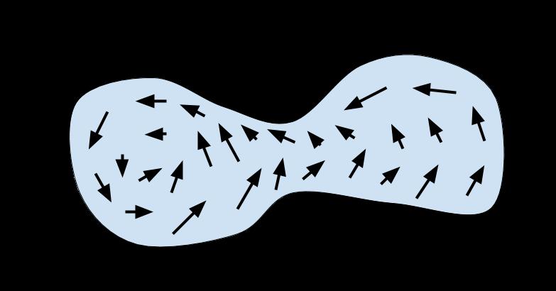
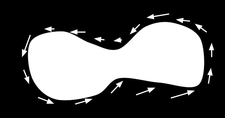
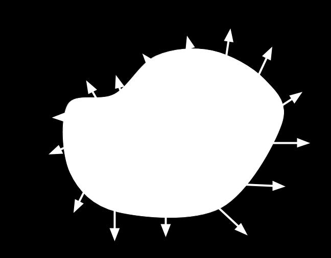
310 Intuition: 16.8 STOKES THEOREM