APPLIED ECONOMETRIC TIME SERIES 4TH EDITION

Transcription

1 APPLIED ECONOMETRIC TIME SERIES 4TH EDITION Chapter 2: STATIONARY TIME-SERIES MODELS WALTER ENDERS, UNIVERSITY OF ALABAMA Copyright 2015 John Wiley & Sons, Inc.

2 Section 1 STOCHASTIC DIFFERENCE EQUATION MODELS

3 Example of a time-series model m = ρ(1.03) m + (1 ρ) m + ε t * t 0 t 1 t (2.2) 1. Although the money supply is a continuous variable, (2.2) is a discrete difference equation. Since the forcing process {ε t } is stochastic, the money supply is stochastic; we can call (2.2) a linear stochastic difference equation. 2. If we knew the distribution of {ε t }, we could calculate the distribution for each element in the {m t } sequence. Since (2.2) shows how the realizations of the {m t } sequence are linked across time, we would be able to calculate the various joint probabilities. Notice that the distribution of the money supply sequence is completely determined by the parameters of the difference equation (2.2) and the distribution of the {ε t } sequence. 3. Having observed the first t observations in the {m t } sequence, we can make forecasts of m t+1, m t+2,.

4 White Noise E(ε t ) = E(ε t 1 ) = = 0 E(ε t ) 2 = E(ε t 1 ) 2 = = σ 2 [or var(ε t ) = var(ε t 1 ) = = σ 2 ] E(ε t ε t-s ) = E(ε t-j ε t-j-s ) = 0 for all j and s [or cov(ε t, ε t-s ) = cov(ε t-j, ε t-j-s ) = 0] x q = βε t i t i i= 0 A sequence formed in this manner is called a moving average of order q and is denoted by MA(q)

5 2. ARMA MODELS In the ARMA(p, q) model y t = a 0 + a 1 y t a p y t-p + ε t + β 1 ε t β q ε t-q where ε t series are serially uncorrelated shocks The particular solution is: q p i yt= a 0 + βε i t i 1 ail i= 0 i= 1 Note that all roots must lie outside of the unit circle. If this is the case, we have the MA Representation y = c+ cε t i t i i= 0

6 tε Section 3 Stationarity Restrictions for an AR(1) Process STATIONARITY

7

8 Covariance Stationary Series Mean is time-invariant Variance is constant All covariances are constant all autocorrelations are constant Example of a series that are not covariance stationary y t = α + β time y t = y t-1 + ε t (Random Walk)

9 Formal Definition A stochastic process having a finite mean and variance is covariance stationary if for all t and t s, 1. E(y t ) = E(y t-s ) = µ 2. E[(y t µ) 2 ] = E[(y t-s µ) 2 ] or [var(y t ) = var(y t s ) = ] 3. E[(y t µ)(y t-s µ)] = E[(y t-j µ)(y t-j-s µ)] = γ s or cov(y t, y t-s ) = cov(y t-j, y t-j-s ) = γ s where µ, and γ s are all constants.

10 4. STATIONARITY RESTRICTIONS FOR AN ARMA(p, q) MODEL Stationarity Restrictions for the Autoregressive Coefficients

11 Stationarity of an AR(1) Process y t = a 0 + a 1 y t 1 + ε t with an initial condition t t 1 t 1 i t i i= 0 i= 0 y = a a+ ay + aε t i Only if t is large is this stationary: lim y t a 1 a 0 = + 1 i= 0 aε i 1 t i E[(y t µ)(y t-s µ)] = E{[ε t + a 1 ε t 1 + (a 1 ) 2 ε t 2 + ] [ε t-s + a 1 ε t-s 1 + (a 1 ) 2 ε t-s 2 + ]} = σ 2 (a 1 ) s [1 + (a 1 ) 2 + (a 1 ) 4 + ] = σ 2 (a 1 ) s /[1 (a 1 ) 2 ]

12 Let Restrictions for the AR Coefficients p y = a + ay + ε t 0 i t i t i= 1 p so that y = a / 1 a + cε t 0 i i t i i= 1 i= 0 We know that the sequence {c i } will eventually solve the difference equation c i a 1 c i 1 a 2 c i 2 a p c i p = 0 (2.21) If the characteristic roots of (2.21) are all inside the unit circle, the {c i } sequence will be convergent. The stability conditions can be stated succinctly: 1. The homogeneous solution must be zero. Either the sequence must have started infinitely far in the past or the process must always be in equilibrium (so that the arbitrary constant is zero). 2. The characteristic root a 1 must be less than unity in absolute value.

13 A Pure MA Process x = βε t i t i i= 0 1. Take the expected value of x t E(x t ) = E(ε t + β 1 ε t 1 + β 2 ε t 2 + ) = Eε t + β 1 Eε t 1 + β 2 Eε t 2 + = 0 E(x t s ) = E(ε t s + β 1 ε t s 1 + β 2 ε t s 2 + ) = 0 Hence, all elements in the {x t } sequence have the same finite mean (µ = 0). 2. Form var(x t ) as var(x t ) = E[(ε t + β 1 ε t 1 + β 2 ε t 2 + ) 2 ] = σ 2 [1 + (β 1 ) 2 + (β 2 ) 2 + ] As long as Σ(β i ) 2 is finite, it follows that var(x t ) is finite. var(x t s ) = E[(ε t s + β 1 ε t s 1 + β 2 ε t s 2 + ) 2 ] = σ 2 [1 + (β 1 ) 2 + (β 2 ) 2 + ] Thus, var(x t ) = var(x t s ) for all t and t s. Are all autocovariances finite and time independent? E[x t x t s ] = E[(ε t + β 1 ε t 1 + β 2 ε t 2 + )(ε t s + β 1 ε t s 1 + β 2 ε t s 2 + )] = σ 2 (β s + β 1 β s+1 + β 2 β s+2 + ) Restricting the sum β s + β 1 β s+1 + β 2 β s+2 + to be finite means that E(x t x t s ) is finite.

14 The Autocorrelation Function of an AR(2) Process The Autocorrelation Function of an MA(1) Process The Autocorrelation Function of an ARMA(1, 1) Process 5. THE AUTOCORRELATION FUNCTION

15 The Autocorrelation Function of an MA(1) Process Consider y t = ε t + βε t 1. Again, multiply y t by each y t s and take expectations γ 0 = var(y t ) = Ey t y t = E[(ε t + βε t 1 )(ε t + βε t 1 )] = (1 + β 2 )σ 2 γ 1 = cov(y t y t 1 ) = Ey t y t 1 = E[(ε t + βε t 1 )(ε t 1 + βε t 2 )] = βσ 2 and γ s = Ey t y t s = E[(ε t + βε t 1 )(ε t s + βε t s 1 )] = 0 for all s > 1

16

17 The ACF of an ARMA(1, 1) Process: Let y t = a 1 y t 1 + ε t + β 1 ε t 1. Ey t y t = a 1 Ey t 1 y t + Eε t y t + β 1 Eε t 1 y t γ 0 = a 1 γ 1 + σ 2 + β 1 (a 1 +β 1 )σ 2 Ey t y t 1 = a 1 Ey t 1 y t 1 + Eε t y t 1 + β 1 Eε t 1 y t 1 γ 1 = a 1 γ 0 + β 1 σ 2 Ey t y t 2 = a 1 Ey t 1 y t 2 + Eε t y t 2 + β 1 Eε t 1 y t 2 γ 2 = a 1 γ 1. Ey t y t s = a 1 Ey t 1 y t s + Eε t y t s + β 1 Eε t 1 y t s γ s = a 1 γ s 1

18 ACF of an AR(2) Process Ey t y t = a 1 Ey t 1 y t + a 2 Ey t 2 y t + Eε t y t Ey t y t 1 = a 1 Ey t 1 y t 1 + a 2 Ey t 2 y t 1 + Eε t y t 1 Ey t y t 2 = a 1 Ey t 1 y t 2 + a 2 Ey t 2 y t 2 + Eε t y t 2.. Ey t y t s = a 1 Ey t 1 y t s + a 2 Ey t 2 y t s + Eε t y t s So that γ 0 = a 1 γ 1 + a 2 γ 2 + σ 2 γ 1 = a 1 γ 0 + a 2 γ 1 ρ 1 = a 1 /(1 - a 2 ) γ s = a 1 γ s 1 + a 2 γ s 2 ρ i = a 1 ρ i-1 + a 2 ρ i-2

19 6. THE PARTIAL AUTOCORRELATION FUNCTION

20 PACF of an AR Process y t = a + a 1 y t-1 + ε t y t = a + a 1 y t-1 + a 2 y t-2 + ε t y t = a + a 1 y t-1 + a 2 y t-2 + a 3 y t-3 + ε t The successive estimates of the a i are the partial autocorrelations

21 PACF of a MA(1) y t = ε t + β 1 ε t-1 but ε t-1 = y t-1 - β 1 ε t-2 y t = ε t + β 1 [ y t-1 - β 1 ε t-2 ] = ε t + β 1 y t-1 (β 1 ) 2 ε t-2 y t = ε t + β 1 y t-1 (β 1 ) 2 [y t-2 - β 1 ε t-3 ] It looks like an MA( )

22 or Using Lag Operators y t = ε t + β 1 ε t 1 = (1 + β 1 L)ε t y t /(1 + β 1 L) = ε t Recall y t /(1 a 1 L) = y t + a 1 y t 1 + a 12 y t 2 + a 13 y t 3 + so that β 1 plays the role of a 1 y t /(1 + β 1 L)ε t = y t /[1 ( β 1 )L]ε t = y t β 1 y t 1 + β 12 y t 2 a 13 y t 3 + = ε t or y t =β 1 y t 1 β 12 y t 2 + β 13 y t 3 + = ε t

23 Summary: Autocorrelations and Partial Autocorrelations ACF AR(1) geometric decay MA(q) cuts off at lag q PACF AR(p) Cuts off at lag p MA(1) Geometric Decay

24 For stationary processes, the key points to note are the following: 1. The ACF of an ARMA(p,q) process will begin to decay after lag q. After lag q, the coefficients of the ACF (i.e., the r i ) will satisfy the difference equation (ρ i = a 1 ρ i 1 + a 2 ρ i a p ρ i-p ). 2. The PACF of an ARMA(p,q) process will begin to decay after lag p. After lag p, the coefficients of the PACF (i.e., the f ss ) will mimic the ACF coefficients from the model y t /(1 + β 1 L + β 2 L β q L q ).

25 TABLE 2.1: Properties of the ACF and PACF Process ACF PACF White Noise All ρ s = 0 (s 0) All φ ss = 0 AR(1): a 1 > 0 s Direct exponential decay: ρ s = a φ 1 11 = ρ 1 ; φ ss = 0 for s 2 AR(1): a 1 < 0 s Oscillating decay: ρ s = a φ 1 11 = ρ 1 ; φ ss = 0 for s 2 AR(p) Decays toward zero. Coefficients may oscillate. Spikes through lag p. All φ ss = 0 for s > p. MA(1): β > 0 Positive spike at lag 1. ρ s = 0 for s 2 Oscillating decay: φ 11 > 0. MA(1): β < 0 Negative spike at lag 1. ρ s = 0 for s 2 Geometric decay: φ 11 < 0. ARMA(1, 1) a 1 > 0 ARMA(1, 1) a 1 < 0 ARMA(p, q) Geometric decay beginning after lag1. Sign ρ 1 = sign(a 1 +β) Oscillating decay beginning after lag 1. Sign ρ 1 = sign(a 1 +β) Decay (either direct or oscillatory) beginning after lag q. Oscillating decay after lag 1. φ 11 = ρ 1 Geometric decay beginning after lag 1. φ 11 = ρ 1 and sign(φ ss ) = sign(φ 11 ). Decay (either direct or oscillatory) beginning after lag p.

26 Testing the significance of ρ i Under the null ρ i = 0, the sample distribution of is: approximately normal (but bounded at -1.0 and +1.0) when T is large distributed as a students-t when T is small. The standard formula for computing the appropriate t value to test significance of a correlation coefficient is: t = ρ ˆi T 2 1 ˆ ρ 2 i SD(ρ) = [ ( 1 ρ 2 ) / (T 2) ] 1/2 with df = T 2 In reasonably large samples, the test for the null that ρ i = 0 is simplified to T 1/2. Alternatively, the standard deviation of the correlation coefficient is (1/T) 0.5.

27 Significance Levels A single autocorrelation st.dev(ρ) = [ ( 1 ρ 2 ) / (T 2) ] ½ For small ρ and large T, st.dev( ρ ) is approx. (1/T) 1/2 If the autocorrelation exceeds 2/T 1/2 we can reject the null that r = 0. A group of k autocorrelations: Q= TT ( + 2) ρi /( T k) i= 1 Is a Chi-square with degrees of freedom = k k

28 Model Selection Criteria Estimation of an AR(1) Model Estimation of an ARMA(1, 1) Model Estimation of an AR(2) Model 7. SAMPLE AUTOCORRELATIONS OF STATIONARY SERIES

29 Sample Autocorrelations r s = T t= s+ 1 ( y y)( y y) t T t= 1 t s ( y y) t 2 Form the sample autocorrelations ( s 2 2) k /( ) k = 1 Q= TT+ r T k Test groups of correlations If the sample value of Q exceeds the critical value of χ 2 with s derees of freedom, then at least one value of r k is statistically different from zero at the specified significance level. The Box Pierce and Ljung Box Q-statistics also serve as a check to see if the residuals from an estimated ARMA(p,q) model behave as a white-noise process. However, the degrees of freedom are reduced by the number of estimated parameters

30 Model Selection AIC = T ln(sum of squared residuals) + 2n SBC = T ln(sum of squared residuals) + n ln(t) where n = number of parameters estimated (p + q + possible constant term) T = number of usable observations. ALTERNATIVE AIC * = 2ln(L)/T + 2n/T SBC * = 2ln(L)/T + n ln(t)/t where n and T are as defined above, and L =maximized value of the log of the likelihood function. For a normal distribution, 2ln(L) = Tln(2π) +Tln(σ 2 ) + (1/σ 2 ) (sum of squared residuals)

31 Figure 2.3: ACF and PACF for two simulated processes 1.00 Panel a: ACF for the AR(1) Process 1.00 Panel b: PACF for the AR(1) Process Panel c: ACF for the ARMA(1,1) Process 1.00 Panel d: PACF for the ARM1(1,1) Process

32 Table 2.2: Estimates of an AR(1) Model Model 1 Model 2 y t = a 1 y t-1 + e t y t = a 1 y t-1 + e t + b 12 e t-12 Degrees of Freedom Sum of Squared Residuals Estimated a 1 (standard error) Estimated b (standard error) (0.0624) (0.0643) (0.1141) AIC / SBC AIC = ; SBC = AIC = ; SBC = Ljung-Box Q- Q(8) = 6.43 (0.490) Q(8) = 6.48 (0.485) statistics for the Q(16) = (0.391) Q(16) = (0.400) residuals Q(24) = (0.536) Q(24) = (0.547) (significance level in parentheses)

33 Figure 2.4: ACF of the Residuals from Model 1

34 Table 2.3: Estimates of an ARMA(1,1) Model Estimates Q-Statistics AIC / SBC Model 1 a 1 : (.053) Q(8) = (.000) Q(24) = (.001) AIC = SBC = Model 2 a 1 : (.076) b 1 : (.081) Model 3 a 1 : (.093) a 2 : (.092) Q(8) = 3.86 (.695) Q(24) = (.892) Q(8) = (.057) Q(24) = (.424) AIC = SBC = AIC = SBC = 487.9

35 ACF of Nonstationary Series Differences CORRS PARTIALS

36 Parsimony Stationarity and Invertibility Goodness of Fit Post-Estimation Evaluation 8. BOX JENKINS MODEL SELECTION

37 Box Jenkins Model Selection Parsimony Extra AR coefficients reduce degrees of freedom by 2 Similar processes can be approximated by very different models Common Factor Problem y t = ε t and y t = 0.5 y t-1 + ε t - 0.5ε t-1 Hence: All t-stats should exceed 2.0 Model should have a good fit as measured by AIC or BIC (SBC)

38 Box-Jenkins II Stationarity and Invertibility t-stats, ACF, Q-stats, all assume that the process is stationary Be suspicious of implied roots near the unit circle Invertibility implies the model has a finite AR representation. No unit root in MA part of the model Diagnostic Checking Plot residuals look for outliers, periods of poor fit Residuals should be serially uncorrrelated Examine ACF and PACF of residuals Overfit the model Divide sample into subperiods F = (ssr ssr 1 ssr 2 )/(p+q+1) / (ssr 1 + ssr 2 )/(T-2p-2q-2)

39 Residuals Plot 1500 Deviations from Trend GDP What can we learn by plotting the residuals? What if there is a systematic pattern in the residuals?

40 Requirements for Box-Jenkins Successful in practice, especially short term forecasts Good forecasts generally require at least 50 observations more with seasonality Most useful for short-term forecasts You need to detrend the data. Disadvantages Need to rely on individual judgment However, very different models can provide nearly identical forecasts

41 Higher-Order Models Forecast Evaluation The Granger Newbold Test The Diebold Mariano Test 9. PROPERTIES OF FORECASTS

42 Forecasting with ARMA Models The MA(1) Model y t = β 0 + β 1 ε t-1 + ε t Updating 1 period: y t+1 = β 0 + β 1 ε t + ε t+1 Hence, the optimal 1-step ahead forecast is: E t y t+1 = β 0 + β 1 ε t Note: E t y t+j is a short-hand way to write the conditional expectation of y t+j The 2-step ahead forecast is: E t y t+2 = E t [ β 0 + β 1 ε t+1 + ε t+2 ] = β 0 Similarly, the n-step ahead forecasts are all β 0

43 Forecast errors The 1-step ahead forecast error is: y t+1 - E t y t+1 = β 0 + β 1 ε t + ε t+1 - β 0 - β 1 ε t = ε t+1 Hence, the 1-step ahead forecast error is the "unforecastable" portion of y t+1 The 2-step ahead forecast error is: y t+2 - E t y t+2 = β 0 + β 1 ε t+1 + ε t+2 - β 0 = β 1 ε t+1 + ε t+2 Forecast error variance The variance of the 1-step ahead forecast error is: var(ε t+1 ) = σ 2 The variance of the 2-step ahead forecast error is: var(β 1 ε t+1 + ε t+2 ) = (1 + β 12 )σ 2 Confidence intervals The 95% confidence interval for the 1-step ahead forecast is: β 0 + β 1 ε t ± 1.96σ The 95% confidence interval for the 2-step ahead forecast is: β 0 ± 1.96(1 + β 12 ) 1/2 σ In the general case of an MA(q), the confidence intervals increase up to lag q.

44 The AR(1) Model: y t = a 0 + a 1 y t-1 + ε t. Updating 1 period, y t+1 = a 0 + a 1 y t + ε t+1, so that E t y t+1 = a 0 + a 1 y t [ * ] The 2-step ahead forecast is: E t y t+2 = a 0 + a 1 E t y t+1 and using [ * ] E t y t+2 = a 0 + a 0 a 1 + a 12 y t It should not take too much effort to convince yourself that: E t y t+3 = a 0 + a 0 a 1 + a 0 a a 13 y t and in general: E t y t+j = a 0 [ 1 + a 1 + a a 1 j-1 ] + a 1j y t If we take the limit of E t y t+j we find that E t y t+j = a 0 /(1 - a 1 ). This result is really quite general; for any stationary ARMA model, the conditional forecast of y t+j converges to the unconditional mean.

45 Forecast errors The 1-step ahead forecast error is: y t+1 E t y t+1 = a 0 + a 1 y t + ε t+1 - a 0 - a 1 y t = ε t+1 The 2-step ahead forecast error is: y t+2 - E t y t+2. Since y t+2 = a 0 + a 1 a 0 + a 12 y t + ε t+2 + a 1 ε t+1 and E t y t+2 = a 0 + a 1 a 0 + a 12 y t, it follows that: y t+2 - E t y t+2 = ε t+2 + a 1 ε t+1 Continuing is this fashion, the j-step ahead forecast error is : y t+j - E t y t+j = ε t+j + a 1 ε t+j-1 + a 12 ε t+j-2 + a 13 ε t+j a 1 j-1 ε t+1 Forecast error variance: The j-step ahead forecast error variance is: σ 2 [ 1 + a a a a 1 2(j-1) ] The variance of the forecast error is an increasing function of j. As such, you can have more confidence in short-term forecasts than in long-term forecasts. In the limit the forecast error variance converges to σ 2 /(1-a 12 ); hence, the forecast error variance converges to the unconditional variance of the {y t } sequence.

46 Confidence intervals The 95% confidence interval for the 1-step ahead forecast is: a 0 + a 1 y t ± 1.96σ Thus, the 95% confidence interval for the 2-step ahead forecast is: a 0 (1+a 1 ) + a 12 y t ± 1.96σ(1+a 12 ) 1/2.

47 Forecast Evaluation Out-of-sample Forecasts: 1. Hold back a portion of the observations from the estimation process and estimate the alternative models over the shortened span of data. 2. Use these estimates to forecast the observations of the holdback period. 3. Compare the properties of the forecast errors from the two models. Example: 1. If {y t } contains a total of 150 observations, use the first 100 observations to estimate an AR(1) and an MA(1) and use each to forecast the value of y 101. Construct the forecast error obtained from the AR(1) and from the MA(1). 2. Reestimate an AR(1) and an MA(1) model using the first 101 observations and construct two more forecast errors. 3. Continue this process so as to obtain two series of one-step ahead forecast errors, each containing 50 observations.

48 A regression based method to assess the forecasts is to use the 50 forecasts from the AR(1) to estimate an equation of the form y 100+t = a 0 + a 1 f 1t + v 1t If the forecasts are unbiased, an F-test should allow you to impose the restriction a 0 = 0 and a 1 = 1. Repeat the process with the forecasts from the MA(1). In particular, use the 50 forecasts from the MA(1) to estimate y 100+t = b 0 + b 1 f 2t + v 2t t = 1,, 50 If the significance levels from the two F-tests are similar, you might select the model with the smallest residual variance; that is, select the AR(1) if var(v 1t ) < var(v 2t ). Instead of using a regression-based approach, many researchers would select the model with the smallest mean square prediction error (MSPE). If there are H observations in the holdback periods, the MSPE for the AR(1) can be calculated as H 1 2 MSPE = e 1i H i = 1

49 The Diebold Mariano Test Let the loss from a forecast error in period i be denoted by g(e i ). In the typical case of mean-squared errors, the loss is e t 2 We can write the differential loss in period i from using model 1 versus model 2 as d i = g(e 1i ) g(e 2i ). The mean loss can be obtained as H 1 d= ge ge H i = 1 [ ( ) ( )] 1i 2i If the {d i } series is serially uncorrelated with a sample variance of γ 0, the estimate of var(d ) is simply γ 0 /(H 1). The expression d / γ /( H 1) 0 has a t-distribution with H 1 degrees of freedom

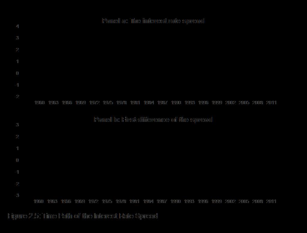
50 Out-of-Sample Forecasts 10. A MODEL OF THE INTEREST RATE SPREAD

51

52 Autocorrelations PA CF Figure 2.6: ACF and PACF of the Spread

53 Table 2.4: Estimates of the Interest Rate Spread AR(7) AR(6) AR(2) p = 1, 2, and 7 ARMA(1, 1) ARMA(2, 1) p = 2 ma = (1, 7) µ y (6.57) (7.55) (6.02) (6.80) (6.16) (5.56) (5.74) a (15.76) (15.54) (15.25) (14.83) (14.69) (2.78) (3.15) a (-4.33) (-4.11) (-3.18) (-2.80) (2.19) (3.52) a (3.68) (3.39) a (-2.70) (-2.30) a (2.02) (1.53) a (-2.86) (-2.11) a (1.93) (-0.77) β (5.23) (5.65) (9.62) β (-3.27) SSR AIC SBC Q(4) Q(8) Q(12)

54 Models of Seasonal Data Seasonal Differencing 11. SEASONALITY

55 Seasonality in the Box-Jenkins framework Seasonal AR coefficients y t = a 1 y t-1 +a 12 y t-12 + a 13 y t-13 y t = a 1 y t-1 +a 12 y t-12 + a 1 a 12 y t-13 (1 a 1 L)(1 a 12 L 12 )y t Seasonal MA Coefficients Seasonal differencing: y t = y t y t-1 versus 12 y t = y t y t-12 NOTE: You do not difference 12 times In RATS you can use: dif(sdiffs=1) y / sdy

56

57 Panel a: M1 Growth Autocorrelations PACF Figure 2.8: ACF and PACF

58 Three Models of Money growth Model 1: AR(1) with Seasonal MA m t = a 0 + a 1 m t 1 + ε t + β 4 ε t 4 Model 2: Multiplicative Autoregressive m t = a 0 + (1 + a 1 L)(1 + a 4 L 4 )m t 1 + ε t Model 3: Multiplicative Moving Average m t = a 0 + (1 + β 1 L)(1 + β 4 L 4 )ε t

59 Table 2.5 Three Models of Money Growth a (8.59) Model 1 Model 2 Model (7.66) a ( 7.28) β (6.84) β ( 15.11) ( 14.87) SSR AIC SBC Q(4) Q(8) Q(12) 1.39 (0.845) 6.34 (0.609) (0.279) 3.97 (0.410) (0.002) (0.001) (0.000) (0.000) (0.000)

60 M1 in Billions Forecasts Figure 2.9: Forecasts of M1

61 Testing for Structural Change Endogenous Breaks Parameter Instability An Example of a Break 12. PARAMETER INSTABILITY AND STRUCTURAL CHANGE

62 Parameter Instability and the CUSUMs Brown, Durbin and Evans (1975) calculate whether the cumulated sum of the forecast errors is statistically different from zero. Define: CUSUM N = ei(1) / σ e N i= n N = n,, T 1 n = date of the first forecast error you constructed, σ e is the estimated standard deviation of the forecast errors. Example: With 150 total observations (T = 150), if you start the procedure using the first 10 observations (n = 10), 140 forecast errors (T n) can be created. Note thatσ e is created using all T n forecast errors. To create CUSUM 10, use the first ten observations to create e 10 (1)/σ e. Now let N = 11 and create CUSUM 11 as [e 10 (1)+e 11 (1)]/σ e. Similarly, CUSUM T-1 = [e 10 (1)+ +e T-1 (1)]/σ e. If you use the 5% significance level, the plot value of each value of CUSUM N should be within a band of approximately ± [ (T n) (N n) (T n) -0.5 ].

63 Figure 2.10: Recursive Estimation of the Model 12 Panel 1: The Series 7 Panel 2: Intercept Intercept + 2 sds. - 2 stds. 2.0 Panel 3: AR(1) Coefficient 50 Panel 4: The CUSUM TEST AR(1) + 2 sds. - 2 stds. CUSUMS Upper 5% Lower 5%

64 Section 13 COMBINING FORECASTS

65 13 Combining Forecasts Consider the composite forecast f ct constructed as weighted average of the individual forecasts f ct = w 1 f 1t + w 2 f 2t + + w n f nt (2.71) and w i = 1 If the forecasts are unbiased (so that E t 1 f it = y t ), it follows that the composite forecast is also unbiased: E t 1 f ct = w 1 E t-1 f 1t + w 2 E t 1 f 2t + + w n E t 1 f nt = w 1 y t + w 2 y t + + w n y t = y t

66 A Simple Example To keep the notation simple, let n = 2. Subtract y t from each side of (2.71) to obtain f ct y t = w 1 (f 1t y t ) + (1 w 1 )(f 2t y t ) Now let e 1t and e 2t denote the series containing the one-step-ahead forecast errors from models 1 and 2 (i.e., e it = y t f it ) and let e ct be the composite forecast error. As such, we can write e ct = w 1 e 1t + (1 w 1 )e 2t The variance of the composite forecast error is var(e ct ) = w 12 var(e 1t ) + (1 w 1 ) 2 var(e 2t ) + 2w 1 (1 w 1 )cov(e 1t e 2t ) (2.72) Suppose that the forecast error variances are the same size and that cov(e 1t e 2t ) =0. If you take a simple average by setting w 1 = 0.5, (2.72) indicates that the variance of the composite forecast is 25% of the variances of either forecast: var(e ct ) = 0.25var(e 1t ) = 0.25var(e 2t ).

67 Optimal Weights var(e ct ) = (w 1 ) 2 var(e 1t ) + (1 w 1 ) 2 var(e 2t ) + 2w 1 (1 w 1 )cov(e 1t e 2t ) Select the weight w 1 so as to minimize var(e ct ): δ var( ect ) δ w 1 = 2w var( e) 2(1 w) var( e ) + 2(1 2 w)cov( ee ) 1 1t 1 2t 1 1t 2t Bates and Granger (1969), recommend constructing the weights excluding the covariance terms. w var( e ) var( e ) 1 * 2t 1t 1 = = 1 1 var( e1 t) + var( e2t) var( e1 t) + var( e2t) In the n-variable case: w var( e ) 1 * 1t n = var( e1 t ) + var( e2t ) var( ent )

68 Alternative methods Consider the regression equation y t = α 0 + α 1 f 1t + α 2 f 2t + + α n f nt + v t (2.75) It is also possible to force α 0 = 0 and α 1 + α α n = 1. Under these conditions, the α i s would have the direct interpretation of optimal weights. Here, an estimated weight may be negative. Some researchers would reestimate the regression without the forecast associated with the most negative coefficient. Granger and Ramanathan recommend the inclusion of an intercept to account for any bias and to leave the α i s unconstrained. As surveyed in Clemen (1989), not all researchers agree with the Granger Ramanathan recommendation and a substantial amount of work has been conducted so as to obtain optimal weights.

69 The SBC Let SBC i be the SBC from model i and let SBC * be the SBC from the best fitting model. Form α i = exp[(sbc * SBC i )/2] and then construct the weights n * i = i / i t= 1 w α α Since exp(0) = 1, the model with the best fit has the weight 1/Σα i. Since α i is decreasing in the value of SBC i, models with a poor fit with have smaller weights than models with large values of the SBC.

70 Example of the Spread I estimated seven different ARMA models of the interest rate spread. The data ends in April 2012 and if I use each of the seven models to make a one-stepahead forecast for January 2013: AR(7) AR(6) AR(2) AR( 1,2,7 ) ARMA(1,1) ARMA(2,1) ARMA(2, 1,7 ) f i2013: Simple averaging of the individual forecasts results in a combined forecast of Construct 50 1-step-ahead out-of-sample forecasts for each model so as to obtain AR(7) AR(6) AR(2) AR( 1,2,7 ) ARMA(1,1 ARMA(2,1) ARMA(2, 1,7 ) ) var(e it ) w i

71 Next, use the spread (s t ) to estimate a regression in the form of (5). If you omit the intercept and constrain the weights to unity, you should obtain: s t = 0.55f 1t 0.25f 2t 2.37f 3t f 4t f 5t 0.28f 6t f 7t (6) Although some researchers would include the negative weights in (6), most would eliminate those that are negative. If you successively reestimate the model by eliminating the forecast with the most negative coefficient, you should obtain: s t = 0.326f 4t f 5t f 7t The composite forecast using the regression method is: 0.326(0.687) (0.729) (0.799) = If you use the values of the SBC as weights, you should obtain: AR(7) AR(6) AR(2) AR( 1,2,7 ) ARMA(1,1) ARMA(2,1) ARMA(2, 1,7 ) w i The composite forecast using SBC weights is In actuality, the spread in 2013:1 turned out to be 0.74 (the actual data contains only two decimal places). Of the four methods, simple averaging and weighting by the forecast error variances did quite well. In this instance, the regression method and constructing the weights using the SBC provided the worst composite forecasts.

72 APPENDIX 2.1: ML ESTIMATION OF A REGRESSION 1 2 2πσ ε exp 2 σ 2 t 2 T 2 1 ε t exp 2 2 t = 1 2πσ 2 σ T T 1 ln L = ln(2 π) lnσ ε Let ε t = y t bx t T T T t σ t = 1 T 2 2 ln L= ln (2 π) ln σ ( ) 2 yt βxt 2 2 2σ t= 1 1 T ln L T 1 = + ( ) yt β xt σ 2σ 2σ t= 1 2 ln L 1 = y 2 x x β σ T 2 ( t t β t) t= 1

73 ML ESTIMATION OF AN MA(1) Now let y t = βε t 1 + ε t. The problem is to construct the {ε t } sequence from the observed values of {y t }. If we knew the true value of β and knew that ε 0 = 0, we could construct ε 1,, ε T recursively. Given that ε 0 = 0, it follows that: ε 1 = y 1 ε 2 = y 2 βε 1 = y 2 βy 1 ε 3 = y 3 βε 2 = y 3 β (y 2 βy 1 ) ε 4 = y 4 βε 3 = y 4 β [y 3 β (y 2 βy 1 ) ] In general, ε t = y t βε t 1 so that if L is the lag operator t 1 i t= yt/(1 + L) = ( ) yt i i= 0 T t 1 2 T T 2 1 i ln L= ln(2 π) lnσ 2 ( β) yt i 2 2 2σ t= 1 i= 0 ε β β