Power System Control

Size: px

Start display at page:

Download "Power System Control"

April Nelson
6 years ago
Views:

1 Power System Control Basic Control Engineering Prof. Wonhee Kim School of Energy Systems Engineering, Chung-Ang University

2 2 Contents Why feedback? System Modeling in Frequency Domain System Modeling in Time Domain Modeling Converting Time Response Stability Steady-state Error Frequency Response Tracking Controller and Observer

3 3 Contents Why feedback? System Modeling in Frequency Domain System Modeling in Time Domain Modeling Converting Time Response Stability Steady-state Error Frequency Response Tracking Controller and Observer

4 4 Open-loop Control vs. Closed-loop Control Open-loop control 100 System 90 (not 100!!)

5 5 Open-loop Control vs. Closed-loop Control Open-loop control 100 System 90 (not 100!!) Closed-loop control System Negative feedback 90

6 6 Open-loop Control vs. Closed-loop Control Open-loop control 100 System 90 (not 100!!) Closed-loop control System 90 = Negative feedback 90

7 7 Open-loop Control vs. Closed-loop Control Open-loop control 100 System 90 (not 100!!) Closed-loop control System 99 - =90+9 Negative feedback 99

8 8 Open-loop Control vs. Closed-loop Control Open-loop control 100 System 90 (not 100!!) Closed-loop control System 99 = =90+9 Negative feedback 99

9 9 Open-loop Control vs. Closed-loop Control Open-loop control 100 System 90 (not 100!!) Closed-loop control System = Negative feedback 99.9

10 10 Open-loop Control vs. Closed-loop Control Vel. ref. + - Input System Vel. output

11 11 Open-loop Control vs. Closed-loop Control Ref. + - Controller System Output Ref. Controller System Output

12 12 Open-loop Control vs. Closed-loop Control Fig. Temperature control system

13 Design Procedure 13

14 Design Procedure (Example) 14

15 Design Procedure (Example) 15

16 Design Procedure (Example) 16

17 Design Procedure (Example) 17

18 18 Design Procedure (Example) Transient response Steady-state response

19 19 Contents Why feedback? System Modeling in Frequency Domain System Modeling in Time Domain Modeling Converting Time Response Stability Steady-state Error Frequency Response Tracking Controller and Observer

20 20 Laplace Transform Review - Laplace transform - Inverse Laplace transform

21 Laplace Transform Review 21

22 Laplace Transform Review 22

23 Laplace Transform Review: - Solution of a Differential Equation Example 1) 23

24 24 System Modeling in Frequency Domain u(t) y(t) u(t) y(t) From input to output: Convolution t * y h u t h u t d 0

25 25 System Modeling in Frequency Domain Laplace transform u(t) y(t) U(s) Y(s) t * y h u t h u t d 0 HsUs Y s Transfer function Y s U s H s

26 26 System Modeling in Frequency Domain Laplace transform u(t) y(t) U(s) Y(s) t * y h u t h u t d 0 Example 2) dy t 2y t u t dt sy s sy s U s Ys 1 Us s 2 H s HsUs Y s

27 Electrical Network Transfer Functions 27

28 Electrical Network Transfer Functions Example 3) 28

29 29 Electrical Network Transfer Functions Example 3) For the capacitor: For the resistor: For the inductor: Impedance: it Cdv t / dt I s C scv s

30 Translational Mechanical System Transfer Functions 30

31 Rotational Mechanical System Transfer Functions 31

32 32 Contents Why feedback? System Modeling in Frequency Domain System Modeling in Time Domain Modeling Converting Time Response Stability Steady-state Error Frequency Response Tracking Controller and Observer

33 33 System Modeling in Time Domain Example 4) Loop equation: I s Vs Ls R

34 34 System Modeling in Time Domain Example 4) Loop equation: Input State variable I s Vs Ls R State equation: Output

35 35 System Modeling in Time Domain Example 5) Loop equation: Not first order differential equation!

36 36 System Modeling in Time Domain Example 5) Loop equation: Input State equation: State variable it, qt Output

37 37 System Modeling in Time Domain Example 5) Loop equation: Input State equation: State variable v t, v t C R

38 38 System Modeling in Time Domain Example 5) State variable: v t, v t or it, qt C R Input State variables must be linearly independent! Linearly dependent: ex) State variable definition v t, i t R v t, v t C it R, qt

39 39 System Modeling in Time Domain Example 5) State variable: v t, v t or it, qt C R Input State variables must be linearly independent! Linearly dependent: ex) State variable definition v t, i t R v t, v t C it R, qt

40 40 System Modeling in Time Domain Example 5) State-space equation:

41 41 System Modeling in Time Domain Example 5) State-space equation: State-space equation

42 42 System Modeling in Time Domain Example 5) State-space equation: x v v R C Fig. Graphic representation of state space and a state vector

43 43 System Modeling in Time Domain State-space equation: State-space equation State equation Output equation This representation of a system provides complete knowledge of all variables of the system at any t t 0.

44 44 System Modeling in Time Domain State-space equation: 2nd order single-input single-output state-space equation: The choice of state variables for a given system is not unique.

45 45 System Modeling in Time Domain State-space equation: How do we know the minimum number of state variables to select?

46 46 System Modeling in Time Domain State-space equation: How do we know the minimum number of state variables to select? Typically, the minimum number required equals the order of the differential equation describing the system. State variable it, qt

47 47 Contents Why feedback? System Modeling in Frequency Domain System Modeling in Time Domain Modeling Converting Time Response Stability Steady-state Error Frequency Response Tracking Controller and Observer

48 48 Converting from Transfer Function to State Space Differential equation State variables and state equation (Phase variable form):

49 49 Converting from Transfer Function to State Space Differential equation State-space equation (Phase variable form): Converting is not unique!

50 50 Converting from Transfer Function to State Space Example 6)

51 51 Converting from Transfer Function to State Space Example 6)

52 52 Converting from State Space to a Transfer Function State-space equation Laplace transform assuming zero initial conditions Transfer Function

53 53 Converting from State Space to a Transfer Function Example 7)

54 54 Converting from State Space to a Transfer Function Example 7)

55 55 Linear System and Nonlinear System 1) Linear systems: - Linear time-invariant system x t Ax t Bu t t C t D t y x u - Linear time-varying system x t A t x t B t u t t C t t D t t y x u 2) Nonlinear systems: - Nonlinear time-invariant system x t f x t,u t t g t t y x,u - Nonlinear time-varying system x t f x t,u t, t t y t g x t,u, t Y s Ts CsI A 1 BD U s Y s Ts CsI A 1 BD U s Y s Ts CsI A 1 BD U s Y s Ts CsI A 1 BD U s

56 56 Linear System and Nonlinear System 1) Linear systems: - Linear time-invariant system x t Ax t Bu t t C t D t y x u x 2xu y x - Linear time-varying system x t A t x t B t u t t C t t D t t y x u 2) Nonlinear systems: - Nonlinear time-invariant system x t f x t,u t t g t t y x,u - Nonlinear time-varying system x t f x t,u t, t 3 t y t g x t,u, t x 2t xu y x x x u y x 3 t x x e u y x

57 57 Contents Why feedback? System Modeling in Frequency Domain System Modeling in Time Domain Modeling Converting Time Response Stability Steady-state Error Frequency Response Tracking Controller and Observer

58 58 Time Response - Pole: Roots of denominator in Transfer function - Zero: Roots of numerator in Transfer function - Step response: Response with step input Example 8) G s s s 2 5 Pole = -5, Zero = -5

59 59 Time Response Example 8) Step response:

60 60 Time Response Example 8) c lim scs c s Steady-state response Transient response

61 61 Time Response Example 9) K K e K e K e 2t 4t 5t

62 62 Time Response: Step response of 1 st order system Rising time: Settling time (0.98):

63 Time Response: Step response of 2 nd order system 63

64 64 Time Response: Step response of 2 nd order system Damped frequency of oscillation, ω d

65 Time Response: Step response of 2 nd order system 65

66 Time Response: Step response of 2 nd order system 66

67 Time Response: Step response of 2 nd order system 67

68 Time Response: Underdamped 2 nd order system 68

69 Time Response: Underdamped 2 nd order system 69

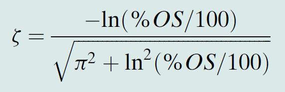
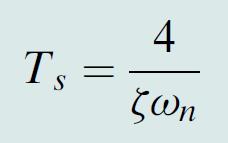
70 70 Time Response: Underdamped 2 nd order system - Rising time T r - Peak time T p - Percent overshoot %OS - Settling time T s

71 Time Response: Underdamped 2 nd order system 71

72 72 Time Response: System response with additional poles Example 10) If the real pole is five times farther to the left than the dominant poles, the system is represented by its dominant second-order pair of poles.

73 73 Time Response: System response with zeros The closer the zero is to the dominant poles, the greater its effect on the transient response. As the zero moves away from the dominant poles, the response approaches that of the two-pole system

74 74 Time Response: System response with zeros - - As the zero moves away from the dominant poles, the response approaches that of the two-pole system

75 75 Time Response: System response with zeros - Nonminimum-phase system: System with negative zero a < 0

76 76 Time Response: Pole-zero cancellation - Pole-zero cancellation: Example 11)

77 77 MATLAB Example: Definition - P1= [ ]; s 3 + 7s 2-3s+23 - P2=poly([ ]); (s+2)(s+5)(s+6) - rootsp2=roots(p2); roots of P2: -2, -5, -6 - P5=conv([ ],[ ]); (s 3 +7s 2 +10s+9)(s 4-3s 3 +6s 2 +2s+l) - A = [1 2; 3 4]; 2 by 2 matrix A [1 2] [3 4]

78 78 MATLAB Example: Transfer function - numf=150*[1 2 7]; denf=[ ]; F=tf (numf, denf); F = 150 (s 2 +2s+7)/(s 3 +5s 2 +4s) - numg=[-2-4]; deng=[ ]; K=20; G=zpk(numg,deng,K); G = 20 [(s+2)(s+4)]/[(s+7)(s+8)(s+9) - s=tf( s ); F=150*(s^2+2*s+7)/[s*(s^2+5*s+4)]; F=150*(s 2 +2s+7)/[s(s 2 +5s+4)]

79 79 MATLAB Example: Converting - num=24 den=[ ] [A,B,C,D]=tf2ss(num,den) - A=[0 1 0;0 0 1; ]; B=[7;8;9]; C=[2 3 4]; D=0; [num,den]=ss2tf(a,b,c,d,1); - Tss=ss(A,B,C,D);

80 80 MATLAB Example: Step Response - numt=[73.626] p1=[ ]; Step Response p2=[1 3]; dent=conv(p1,p2); Amplitude T=tf(numt,dent); step(t); Time (sec) Step Response t=0:0.1:10; step(t,t) Amplitude Time (sec)

81 81 Contents Why feedback? System Modeling in Frequency Domain System Modeling in Time Domain Modeling Converting Time Response Stability Steady-state Error Frequency Response Tracking Controller and Observer

82 82 Stability System response: From input From system -Stable: - Unstable: - Marginally stable: natural t limc 0 t natural natural limc t or limc t t natural t natural limc t aor limc t a t t A system is stable if every bounded input yields a bounded output. The bounded-input, bounded-output (BIBO) definition of stability.

83 83 Stability in Transfer Function Example 12) c lim scs c s Stable systems have closed-loop transfer functions with poles only in the left half-plane.

84 84 Closed-loop System Open-loop control R(s) G(s) C(s) C s R s G s Closed-loop control R(s) + - P(s) C(s) C s R s P s Gs 1 P s

85 85 Stability of Closed-loop System Example 13) C s R s G s 1 G s 3 3 s 3s2s s 3s 2s 3 3 s 3s2s3 C s R s G s 1 G s 7 3 s 3s2s s 3s 2s 7 3 s 3s2s7

86 86 Stability of Closed-loop System Example 14)

87 87 Stability: Routh-Hurwitz criterion A system is stable if there are no sign changes in the first column of the Routh table

88 88 Stability: Routh-Hurwitz criterion Example 15) Two poles in the right half plane

89 89 Stability: Controller design in frequency domain R(s) + - P c1 (s) P(s) C(s) P c2 (s) c C s Pc 1 s P 2 s P s R s 1 P s P s P s c1 c2

90 90 Stability: PID Controller design 1 PPID s KP KI KDs s Ps N s D s R(s) + - P PID (s) P(s) C(s) 1 N s KP KI KDs Cs PPID sps s D s Rs 1 PPID sps 1 N s sd s KDs KPsKI N s 1KP KI KDs s D s 2 KDs KPs KINs 2

91 91 MATLAB Simulink Example: Place 5 P = tf(5,[1 10]); Ps s 10 KD = 0.1; KP = 300; KI = 1; Ppid = tf([kd KP KI],[1 0]); PPID s KP KI KDs s G = Ppid*P/(1+Ppid*P) G1 = feedback(ppid*p,1) zero(g1) pole(g1) step(g1) KI Gain2 1 s Integrator 2 1 K Ds KPs KI Scope1 s Step KP Gain Subtract 5 s+10 Transfer Fcn Scope KD Gain1 du/dt Derivative

92 92 Stability in State Space: Eigenvalue and eigenvector Eigenvector Eigenvector For nonzero solution x (a) Not eigenvector (b) Eigenvector

93 93 Stability in State Space: Eigenvalue and eigenvector Example 16)

94 94 Stability in State Space t A t B t t C t D t x x u y x u Y s 1 adj i I A Ts CsI A BDC BD U s det I A i Example 17) The system poles depend on the eigenvalues of A

95 95 Stability in State Space t A t B t t C t D t x x u y x u Solution: State transition matrix: In particular, if the matrix A is diagonal, then

96 Stability: Stats feedback controller design in time domain 96 t A t B t t C t D t x x u y x u u t Kx t t A t BK t A BK x t x x x K should be chosen such that (A-BK) is Hurwitz!

97 97 MATLAB Example: Place - A=[0 1;2 3]; eig(a); A s eigenvalues - p = [-1-5]; A=[0 1;2 3]; B=[1;2]; K = place(a,b,p); K for desired poles

98 98 MATLAB Simulink Example - X_ini = [10;10]; p = [-1-5]; A=[0 1;2 3]; B=[0;2]; C=[1 0]; D=0; K = place(a,b,p); eig(a-b*k) *uvec Gain1 Subtract 1 s Integrator1 Gain3 K*uve Gain4 K*uve *uvec Gain5 Scope

99 Stability: Stats feedback controller design in time domain 99 Regulation) t A t B t t Cx t x t Axt But y t Cx t x x u y Y s Ts CsI A 1 B U s Using final value theorem, steady-state step response becomes If t A t BK t BKrt A BK x t BJr t x x x J u t Kxt Jrt Y s 1 Ts CsI ABK BJ R s z p m 0 k s z s z k s p s p kz szm sz0 kz zmz0 ylim stsrslimtslim J J s0 s0 s0 kp s pn s p0 kp pnp0 kp pn p p k 0 0 zs zms z0 rlim sts Yd slimtslim J 1 s0 s 0 s 0 k z z z 0 kps pns p0 z m 0 n 0

100 100 MATLAB Example: Place - X_ini = [0;0]; p = [-1-5]; A=[0 1;2 3]; B=[0;2]; C=[1 0]; D=0; K = place(a,b,p); eig(a-b*k) [num,den]=ss2tf(a-b*k,b,c,d) F = 5/2; Step F p z 0 0 F Gain2 Subtract1 *uvec Gain1 Subtract 1 s Integrator1 Gain3 K*uve *uvec Gain5 Scope Gain4 K*uve

101 101 Contents Why feedback? System Modeling in Frequency Domain System Modeling in Time Domain Modeling Converting Time Response Stability Steady-state Error Frequency Response Tracking Controller and Observer

102 Steady-state Error: Frequency domain 102

103 103 Steady-state Error: Frequency domain Fig. Steady-state error: a. step input; b. ramp input

104 104 Steady-state Error: Frequency domain R(s) + - E(s) P C (s) P(s) C(s) E s R s C s C s P s P s E s E s e C 1 P lim s0 1 C 1 s P s P C sr s R s s P s

105 105 Steady-state Error: Step response e lim s0 1 P C sr s s P s R s 1 s e 1 1 limp C s0 s P s For lim P C s0 s P s P C s P s s z1 s z2 n s s p1 s p2 Integrator is required to eliminate the steady-state error

106 Steady-state Error: Disturbance 106

107 107 Steady-state Error: Disturbance Increasing G 1 (s) can reduce both e R and e D

108 Steady-state Error: Frequency domain t A t BK t Brt A BK x t Br t x x x E s R s Y s lim lim 1 Y s T s CsI ABK 1 BD R s 1 e se s sr s C si A BK B D s0 s0 1 Rs s s zm s z zm z e lim 1 CsI A BK B D 1lim 1 s0 s0 s p s p p p n 0 n r p z 0 0 r szm sz p 1 0 pn p0 0 e lim 1 C si ABK BD 1lim 11 0 s0 z s0 0 zmz0 s pn s p0

109 109 Contents Why feedback? System Modeling in Frequency Domain System Modeling in Time Domain Modeling Converting Time Response Stability Steady-state Error Frequency Response Tracking Controller and Observer

110 110 Frequency Response Fig. Sinusoidal frequency response: a. system; b. transfer function; c. input and output waveforms

111 111 Frequency Response: Fourier series N a0 2 nr xt xn t Ansin n 2 n1 P

112 112 Frequency Response u(t) y(t)? U(s) Y(s)

113 113 Frequency Response cos sin cos tan / r t A t B t A B t B A (1) Polar form : M where M A B and tan B/ A (2)Rectangular form : A jb i i (3) Euler's forular : Me i i i i i 2 2 1

114 Frequency Response 114

115 115 Frequency Response icos i ct MM cost r t M t i G i G Frequency ω determines the M G and ϕ G.

116 116 Frequency Response Example 18)

117 Frequency Response Plot: Bode plot (Approximation) 117

118 Frequency Response Plot: Bode plot (Approximation) 118

119 119 Frequency Response Plot: Bode plot Fig. Asymptotic and actual normalized and scaled magnitude response of (s + a)

120 120 Frequency Response Plot: Bode plot Fig. Asymptotic and actual normalized and scaled phase response of (s + a)

121 121 Frequency Response Plot: Bode plot (a) s (b) 1/s Fig. Asymptotic and actual normalized and scaled bode plot

122 122 Frequency Response Plot: Bode plot (a) s+a (b) 1/(s+a) Fig. Asymptotic and actual normalized and scaled bode plot

123 123 Frequency Response Plot: Bode plot Example 19) G s s 3 1s 2 s s

124 124 Frequency Response Plot: Bode plot Example 19) G s s 3 1s 2 s s

125 Frequency Response Plot: Bode plot 125

126 Frequency Response Plot: Bode plot 126

127 127 Frequency Response Plot: Bode plot 2 2 1/ 2 n n G s s s

128 128 Frequency Response Plot: Bode plot 2 2 1/ 2 n n G s s s

129 129 Relationship of Frequency and Time Response 2 2 1/ 2 n n G s s s

130 System Modeling and Analysis in Frequency Domain 130

131 System Modeling and Analysis in Frequency Domain 131

132 Gain Margin and Phase Margin for Closed-loop Stability 132 R(s) + - E(s) P C (s) P(s) C(s) Open-loop : P C Closed-loop : 1 s Ps PC sps P sps C

133 Gain Margin and Phase Margin for Closed-loop Stability 133 Fig. Bold plot of open-loop system

134 134 MATLAB Example: Bode plot - G = tf([1 3],[ ]); bode(g); 60 Bode Diagram 40 Magnitude (db) Phase (deg) Frequency (rad/sec)

135 Gain Margin and Phase Margin for Closed-loop Stability 135 R(s) + - E(s) P C (s) P(s) C(s) Open-loop : P C Closed-loop : 1 s Ps PC sps P sps Reference) C

136 136 Controller Design using Bode Plot sps PC Closed-loop : 1 P s P s C Fig. Bold plot of closed-loop system

137 137 Controller Design using Bode Plot Open-loop : PC s P s Fig. Bold plot of open-loop system

138 138 Contents Why feedback? System Modeling in Frequency Domain System Modeling in Time Domain Modeling Converting Time Response Stability Steady-state Error Frequency Response Tracking Controller and Observer

139 139 Tracking Controller Design 1. System x x x 1 2 x 2 3 x a x a x bu n 1 1 n n 2. Controller design - Aim: x r 1 - Tracking error define: - Tracking Error dynamics e rx e Controller e r x 1 1 n n1 e r x e r x r a x a x bu n 1 n n 1 1 n n 1 n1 u r a1x1a2x2ke 1 1kne b n n e e 1 2 e ke k e n 1 1 n n

140 140 Observer Design 1. System x AxBu y Cx 2. Observer design - Aim: ˆx x - Estimation error define: x x xˆ - Observer xˆ AxˆBuL y yˆ yˆ Cxˆ - Estimation error dynamics x xxˆ AxBu AxˆBuLC xxˆ ALC x

141 141 Tracking Controller Design Example 1. System x x 1 2 x a x a x bu Controller design - Aim: x r 1 - Tracking error define: e r x 1 1 e r x Tracking Error dynamics e rx e e r x r a x a x bu Controller 1 u r a x a x ke k e b Control gain k1, k2 should be designed such that Ac = [0 1; k1 k2] is Hurwitz e e e ke k e

142 142 Observer Design Example 1. System x x 1 2 x a x a x bu Observer design - Aim: xˆ x, xˆ x Estimation error define: x x xˆ x x xˆ Observer xˆ xˆ l y yˆ xˆ l x xˆ xˆ a xˆ a xˆ bul y yˆ a xˆ a xˆ bul x xˆ Estimation error dynamics x x x ˆ x xˆ l y yˆ l x x x x x ˆ a x a x bu a xˆ a xˆ bul x xˆ l a x a x Observer gain l1, l2 should be designed such that Ao=[-l1 1; -l2+a1 a2] is Hurwitz

143 143 Closed-loop Stability Not 1 u r a x a x ke k e b Reference Controller 1 u r a xˆ a xˆ keˆ k eˆ b u x x 1 2 System x a x a x bu Output y x 1 xˆ, xˆ 1 2 Observer xˆ xˆ l x xˆ xˆ a xˆ a xˆ bul x xˆ eˆ rxˆ rx x x e x eˆ r x 2 2

144 144 Closed-loop Stability: Separation Principle 1. Error dynamics e e 1 2 e r a x a x bu u r a xˆ a xˆ keˆ k eˆ b e1 e2 e ke k e a k x a k x Closed-loop system dynamics e e1 e 2 k1 k2 a1k1 a2 k 2 e 2 x1 0 0 l1 1 x1 x2 0 0 l2 a1 a2 x2 X A c A X A o A x is Hurwitz if both A c and A o are Hurwitz so that X converges to zero. This is, each controller gain and observer gain can be designed independently! X

145 145 MATLAB Example: Tracking controller and observer 1. Design the controller and observer for this system x x 1 2 x 10x 5x 2u r t x 10sint , x 0 2 Check about the solver! When sine signal is used, the fixed step is used for the simulation! Setting: Simulation Configuration Type: Fixed step, solver: ODE4

146 146 MATLAB Example: Tracking controller and observer 1. Design the controller and observer for this system % 시스템상수선언 a1= 10; a2 = 5; b = 2; A = [0 1; a1 a2]; B = [0;2]; C = [1 0]; % 초기값선언 x0 = [5 2]; % 추종오차 e의동역학의 pole pole_c = [-50; -50]; % dot e = [0 1; k1 k2]*e --> dot e = A1*e + B1*u u = - Kc * e A1 = [0 1; 0 0]; B1 = [0;1]; Kc = acker(a1,b1,pole_c); k1 = Kc(1); k2 = Kc(2); % 관측오차 tilde x의 pole pole_o = [-100; -100]; % dot tilde x = (A - L*C ) tilde x --> eig(a - L*C) = eig(a' - C'*L') Ko = acker(a',c',pole_o); l1 = Ko(1); l2 = Ko(2); L = [l1;l2]; % pole 확인 eig([0 1; -k1 -k2]) eig([-l1 1; -l2+a1, a2])

147 147 MATLAB Example: Tracking controller and observer 1. Design the controller and observer for this system Sine Wave du/dt Derivative1 [r] Goto du/dt Derivative [dr] Goto1 [ddr] Goto2 [u] From4 *uvec B Gain6 Add Add2 1 s Integrator K*uve A *uvec Gain1 [x] Goto4 [x1] Goto3 Observer Controller Scope4 K*uve [xh1] Goto6 [xh] From [r] From1 [dr] From2 f(u) Fcn [u] Goto7 [r] From5 [x1] Add1 1 s Integrator1 Gain3 K*uve *uvec Gain4 [xh] Goto5 [ddr] From3 From6 [x1] From7 [xh1] From8 Scope Scope1 [x] From9 Scope2 [xh] From10

Power Systems Control Prof. Wonhee Kim. Modeling in the Frequency and Time Domains

Power Systems Control Prof. Wonhee Kim Modeling in the Frequency and Time Domains Laplace Transform Review - Laplace transform - Inverse Laplace transform 2 Laplace Transform Review 3 Laplace Transform