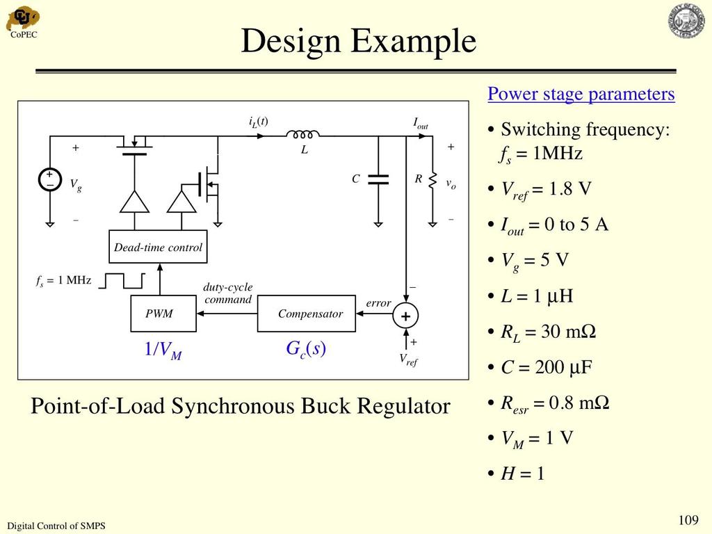
DIGITAL CONTROL OF POWER CONVERTERS. 3 Digital controller design

Size: px

Start display at page:

Download "DIGITAL CONTROL OF POWER CONVERTERS. 3 Digital controller design"

Hester Patterson
6 years ago
Views:

1 DIGITAL CONTROL OF POWER CONVERTERS 3 Digital controller design

2 Frequency response of discrete systems H(z) Properties: z e j T s 1 DC Gain z=1 H(1)=DC 2 Periodic nature j Ts z e jt e s cos( jt ) j sin( jt ) s 3 Symmetry jts jt jts jts s H( e ) H( e ) H( e ) H( e ) jts jts H ( e ) H ( e ) s 2

3 Frequency response of discrete systems 1 DC Gain 2 Periodic nature 3 Symmetry 1 3 Symmetry 2 -Fs/2 0 Fs/2 Fs/2 3

4 Matlab commands for frequency response >> Num = [1 0]; >> Den = [1-1] >> gz = tf(num, den, 0.2) g num( z) den( z) Ts 0.2 g z z 1 Ts 0.2 >> bode(gz) // alternative >> [M, P, w] = bode(gz, w) >> nyquist(gz) // alternative >> [Real, Imag, w] = nyquist(gz, w) 4

5 Discretization of a continous function

6 DAC, Analog Subsystem, and ADC Combination Transfer Function The impulse response is 6

7 DAC, Analog Subsystem, and ADC Combination Transfer Function g s (t) -g s (t-t) g s (T)-g s (t-t) 7

8 PWM, Analog Subsystem, and ADC Combination Transfer Function d k PWM positive step at kt negative step at kt + d k T g s (t) g s (T)-g s (t-d k T) -g s (t-d k T) 8

9 stability of digitally controlled systems 1. The characteristic polynomial 1 + C(z)G ZAS (z) has no zeros on or outside the unit circle. 2. The loop gain C(z)G ZAS (z) has no pole-zero cancellation on or outside the unit circle. 9

10 stability determination (matlab) >> den=[2 1 0]; >> gz=tf(1,den,0.1) Transfer function: z^2 + z >> roots(den) // where den is a vector with the denominator coefficients >> zpk(gz) // factorizes the numerator and denominator of the transfer function gz Zero/pole/gain: z (z+0.5) 10

11 Nyquist criterion >> nyquist(gd) % Nyquist plot >> bode(gd) % Bode plot It is also possible to find the gain and phase margins with the command >> [gm,pm] = margin(gd) An alternative form of the command is >> margin(gd) Z = N + P If G ZAS is stable Stability is assured if R G does not enclosed -1 11

12 Direct z-domain Digital Controller Design Obtaining digital controllers from analog designs involves approximation that may result in significant controller distortion the locations of the controller poles and zeros are often restricted to subsets of the unit circle (s + a) [z (c a)/(c + a)] c=1/2 if a <1/2 This yields only RHP zeros because a is almost always smaller than c 12

13 Direct z-domain design Root locus

14 Direct z-domain Digital Controller Design 1+KL(z)=1 Root locus Magnitude condition K L(z) = 1 Angle condition L(z) = ±(2m + 1)180, m = 0,1,2, The number of root locus branches is equal to the number of open-loop poles of L(s). 2. The root locus branches start at the open-loop poles and end at the open loop zeros or at infinity. 3. The real axis root loci have an odd number of poles plus zeros to their right. 4. The branches going to infinity asymptotically approach the straight lines defined by the angle 5. Breakaway points (points of departure from the real axis) correspond to local maxima of K, whereas break-in points (points of arrival at the real axis) correspond to local minima of K. 6. The angle of departure from a complex pole pn is given by 14

The settling time is defined as the period after which the envelope of the

15 Root locus design Translate time domain info into dominant poles (frequency domain) Settling time. The settling time is defined as the period after which the envelope of the sampled waveform stays within a specified percentage (usually 1 to 2%) 1 Overshoot 0.6 % overshoot (1 ) 100 t s 4 n 2 s s 2 1 n n 15

16 Root locus design Overshoot vs phase margin Translate time domain info into dominant poles (frequency domain) 16

17 Root locus p /T 0.5 p /T 0.4 p /T p /T 0.9 p /T 0.7 p /T p /T p /T 0.1 p /T n =cte =cte 0 p /T p /T p /T 0.1 p /T p /T 0.7 p /T 0.3 p /T 0.2 p /T MATLAB >>zgrid 0.6 p /T 0.4 p /T 0.5 p /T

18 Example 1 Design a discrete controller for the antenna system Ts = 1s overshoot 16% ts < 10 s (ten samples) Gs () 1 s(10s 1) overshoot 16% >0,5 PM>50º ts < 10 s n > 0,9 (/2pi) fc = 0,15 Hz >> Gs = tf([1],[10 1 0]) // generates the transfer function >> Gz=c2d(Gs,1, zoh ) // discretizes Gs with Ts = 1s and zoh >> sisotool (z ) (z-1) (z ) 18

19 Example 1 Original design PM =9º 19

20 Example 1 Original design add a pole to make it causal cancel this pole with a zero PM =9º 20

21 Example 1 Controller design drag the gain to obtain PM=50º bandwidth = 0,1 Hz 21

22 Example 1 Controller design 22

23 Example 1 Controller design If we move this pole to the left (this can only be done in root locus) 23

24 Example 1 Controller design PM=50º bandwidth = 0,16 Hz The phase increases and allows pushing the frequency 24

25 Example 1 Controller design PM=50º bandwidth = 0,16 Hz PM=60º bandwidth = 0,13 Hz just moving the gain 25

26 Example 2 Flyback converter a p c Ve L Co R PWM

27 Fase Módulo Discrete Controller design Converter data Vg= 15V-30V Ls = 20uH Vo = 5v R = 1 C = 600u Resr = 20 m n1:n2 = 2:1 Objective Design the best controller Respuesta en Frecuencia Control-Salida Frecuencia Respuesta en Frecuencia Control-Salida f_rhz = 6.9 khz Frecuencia f_esr = 13.3 khz f_res = 846 Hz 27

28 30 Vin dil L vin d vo (1 d) dt dvc C il (1 d) i dt Converter modelling in Simuling (averaged) o ic v v R ( i (1 d) i ) o C ESR L o -K- Resr Vo Product Gain _L 1 s Integrator _L Product 1 2/1 Trafo _1 ic -K- -K- Gain _C 1 s Vc Integrator _C d 1/1.25 d 1-d G_Rload duty 1 Product 2 2/1 Trafo _2 cte 28

29 add linearization point (input port) to the duty cycle add linearization point (output port) to the output voltage 29

30 Then Tools Control Design linear analysis 30

31 calculate the operating point (default states =0) select Bode plot calculate new operating point 31

32 New operating point Compute operating point 32

33 select the new operating point linearize the model 33

34 default operating point 2nd order with correct operating point RHPZ 34

35 select the correct model export to 35

36 >> flyback_z=c2d(flyback,10e-6,'zoh') >> sisotool Poles discretized flyback converter RHPZ ESRZero 36

1) add integrator 2) place complex conjugates ceros

37 1) add integrator 2) place complex conjugates 3) add additional pole (to make it causal) 37

38 Another way design the compensator from simulink take care about operating point!!! 38

39 Direct z-domain Digital Controller Design

40 Direct z-domain Digital Controller Design Direct Control Design Desired closed loop transfer function The controller is: For a causal controller, the closed-loop transfer function Gcl(z) must have the same pole-zero deficit as GZAS(z). In other words, the delay in Gcl(z) must be at least as long as the delay in GZAS(z) 40

41 Direct z-domain Digital Controller Design Controller requirements Causality: the closed-loop transfer function Gcl(z) must have the same pole-zero deficit as G ZAS (z). In other words, the delay in Gcl(z) must be at least as long as the delay in G ZAS (z) Avoid unstable pole-zero cancellations. This implies that the set of zeros of Gcl(z) must include all the zeros of G ZAS (z) that are outside the unit circle. The zeros of 1 Gcl(z) must include all the poles of G ZAS (z) that are outside the unit circle (stability). zero steady-state error: Gcl(1)=1 Note: The choice of a suitable closed-loop transfer function is clearly the main obstacle in the application of the direct design method. The correct choice of closed-loop poles and zeros to meet the design requirements is difficult for higher order systems. In practice, there are additional constraints on the control variable because of actuator limitations. Further, the performance of the control system relies heavily on an accurate process model. 41

Direct z-domain Digital Controller Design Finite settling time (dead-beat controller) if all the poles and zeros of the discrete-time process are inside

42 Direct z-domain Digital Controller Design Finite settling time (dead-beat controller) if all the poles and zeros of the discrete-time process are inside the unit circle, an attractive choice can be to select Gcl(z) = z k k must be greater than or equal to the intrinsic delay of the discretized process 42

43 Finite settling time Example Ts = 0.1 u output actual analog output To avoid intersample oscillations: maintain the control variable constant after n samples, where n is the degree of the denominator of the discretized process 43

44 44

45 45

46 2.6. Implementation of the controller x k x k-1 x k-m X b 0 X b 1 X b m + + + y k y k-1 y k-n X a 1 X a n + + + - y k n n 2 2 1 1 0 m m 2 2 1 1 0 z a... z a z a a z b.

46 Implementation of the controller x k x k-1 x k-m X b 0 X b 1 X b m y k y k-1 y k-n X a 1 X a n y k n n m m z a... z a z a a z b... z b z b b e(z) d(z) R(z) n k n 1 k 1 m k m 1 k 1 k 0 k d a... d a e b... e b e b d The transfer function R(z) is not implemented, but its equivalent difference equation TF Difference equation (a 0 =1 for normalization)

47 2.6. Canonical form Half memory elements e K R 1 R 2 Z -1 b o dk Half registers (in FPGAs or ASICs) Half variables (in DSPs or Cs) Z -1 b 1 a 1 Z -1 e K R 1 (z) R 2 (z) Y K Z -1 b 2 a 2 Higher values in the registers (more bits) e K b o d K Z -1 a 1 b 1 Z -1 47

48 2.6. Delta transform (I) Y k X k X b o k1 X T k Xk A X s k B U k Difference equation 1 z T 1 b 1 b m e(z) h(z) u(z) a 1 Numerical robustness a 2 a m Less bits are necessary a n More adders X k 1 Y k T z 1 z 1 1 Y k -1 (Integral) Digital implementation T Z

49 2.6. Delta transform (II) Taking out the T multiplier of -1 into the coefficients Adapted -1 Digital implementation -1 b o + Z -1 a 1 T T b 1 a 2 T 2-1 T 2 T n T n b 2 b o is eliminated if order (den) > order (num) The new coefficients are T i a i, T i b i a n =0 if K i 0 (integral action) 49

50 2.6. Order(den) > Orden(num) Really convenient for practical implementation, especially for high f SAMP If order (den) = order (num) d k = b o e k + Duty cycle must be changed (theoretically) at the same time a new sample is received, with a sampled period of (theoretically) 0 ns. If order (den) > order (num) d k = b 1 e k-1 + We have a full cycle for all the process sampling period processing e k-1 is requested e k-1 is available T d k is imposed 50

51 Word length (Number of bits) Coefficients & variables are implemented using fixed point format FPGAs &ASICs allow using any number of bits 1.56 for each variable 1.54 DSPs & Cs use multiples of 8/ Floating point demands too many resources and processing time v o v o allows less number of bits Ideal (floating point) -1 using 8-bits z -1 using 8-bits Low number of bits big differences between ideal model & practical implementation x x 10-4 Matlab fixed-point toolbox 51

Digital Control Systems

Digital Control Systems Lecture Summary #4 This summary discussed some graphical methods their use to determine the stability the stability margins of closed loop systems. A. Nyquist criterion Nyquist