An Overview of Fluid Animation. Christopher Batty March 11, 2014

Transcription

1 An Overview of Fluid Animation Christopher Batty March 11, 2014

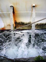
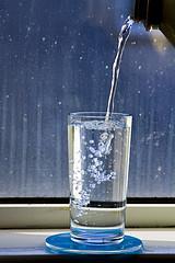
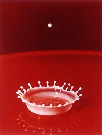
2 What distinguishes fluids?

3 What distinguishes fluids? No preferred shape. Always flows when force is applied. Deforms to fit its container. Internal forces depend on velocities, not displacements (compare v.s., elastic objects)

4 Examples For further detail on today s material, see Robert Bridson s online fluid notes. (There s also a book.)

5 Basic Theory

6 Eulerian vs. Lagrangian Lagrangian: Point of reference moves with the material. Eulerian: Point of reference is stationary. e.g. Weather balloon (Lagrangian) vs. weather station on the ground (Eulerian)

7 Eulerian vs. Lagrangian Consider an evolving scalar field (e.g., temperature). Lagrangian view: Set of moving particles, each with a temperature value.

8 Eulerian vs. Lagrangian Consider an evolving scalar field (e.g., temperature). Eulerian view: A fixed grid of temperature values, that temperature flows through.

9 Relating Eulerian and Lagrangian Consider the temperature T(x, t) at a point following a given path, x(t). x(t 0 ) x(t 1 ) x(t now ) How can temperature measured at x(t) change? 1. There is a hot/cold source at the current point. 2. Following the path, the point moves to a cooler/warmer location.

10 Mathematically: Time derivatives D Dt T T x t, t = t + T x x t Chain rule! = T t = T t + T x t + u T Definition of Choose x t = u

11 Material Derivative This is called the material derivative, and denoted D Dt. (AKA total derivative.) Change at a point moving along the given path, x(t). Change due to movement of the point. DT Dt = T t + u T Change at the current (fixed) point.

12 Advection To track a quantity T moving (passively) through a velocity field: DT Dt = 0 or equivalently T t + u T = 0 This is the advection equation. Think of colored dye or massless particles drifting around in fluid.

13 Advection

14 Equations of Motion For general materials, we have Newton s second law: F = ma. The Navier-Stokes equations are essentially the same equation, specialized to fluids.

15 Navier-Stokes Density Acceleration = Sum of Forces ρ Du Dt = i F i Expanding the material derivative ρ u t = ρ u u + i F i

16 What are the forces on a fluid? Primarily for now: Pressure Viscosity Simple external forces (e.g. gravity, buoyancy, user forces) Also: Surface tension Coriolis Possibilities for more exotic fluid types: Elasticity (e.g. silly putty) Shear thickening / thinning (e.g. oobleck, ketchup, paints) Electromagnetic forces: magnetohydrodynamics, ferrofluids, etc. Sky s the limit...

17 Exotic Fluids - Oobleck

18 Exotic Fluids - Ferrofluid

19 In full ρ u t = ρ u u + i F i Change in velocity at a fixed point Advection (of velocity) Forces (pressure, viscosity gravity, )

20 Operator splitting Break the full, nonlinear equation into substeps: 1. Advection: ρ u t = ρ u u 2. Pressure: ρ u t = F pressure 3. Viscosity: ρ u t = F viscosity 4. External: ρ u t = F other

21 1. Advection

22 Advection Earlier, we considered advection of a passive scalar quantity, T, by velocity u. T t = u T In Navier-Stokes we saw: u t = u u Velocity u is advected by itself!

23 Advection That is, u, v, w components of velocity u are advected as separate scalars. May be able to reuse the same numerical method.

24 2. Pressure

25 Pressure What does pressure do? Enforces incompressibility (fights compression). Typical fluids (mostly) do not compress. Exceptions: high velocity, high pressure,

26 Incompressibility Compressible velocity field Incompressible velocity field

27 Incompressibility Intuitively, net flow into/out of a given region is zero (no sinks/sources). Integrate the flow across the boundary of a closed region: u n = 0 Ω n

28 Incompressibility u n = 0 Ω By divergence theorem: u = 0 But this is true for any region, so u = 0 everywhere. Incompressibility implies u is divergence-free.

29 Pressure Where does pressure come in? Pressure is the force needed to enforce the constraint u = 0. Pressure force has the following form: F p = p

30 Helmholtz Decomposition Input (Arbitrary) Velocity Field Curl-Free (Irrotational) Divergence-Free (Incompressible) = + u = p + φ u old = F pressure + u new

31 Aside: Pressure as Lagrange Multiplier Interpret as an optimization: Find the closest u new to u old where u new = 0 ρ argmin u new 2 u new u old subject to u new = 0 The Lagrange multiplier that enforces the constraint is the pressure. e.g., recall the fast projection paper, Goldenthal et al

32 3. Viscosity

33 High Speed Honey

34 Viscosity What characterizes a viscous liquid? Thick, damped behaviour. Strong resistance to flow.

35 Viscosity Loss of energy due to internal friction between molecules moving at different velocities. Interactions between molecules causes shear stress that opposes relative motion. causes an exchange of momentum.

36 Viscosity Loss of energy due to internal friction between molecules moving at different velocities. Interactions between molecules causes shear stress that opposes relative motion. causes an exchange of momentum.

37 Viscosity Loss of energy due to internal friction between molecules moving at different velocities. Interactions between molecules causes shear stress that opposes relative motion. causes an exchange of momentum.

38 Viscosity Loss of energy due to internal friction between molecules moving at different velocities. Interactions between molecules causes shear stress that opposes relative motion. causes an exchange of momentum.

39 Viscosity Imagine fluid particles with general velocities. Each particle interacts with nearby neighbours, exchanging momentum.

40 Diffusion The momentum exchange is related to: Velocity gradient, u, in a region. Viscosity coefficient, μ. Net effect is a smoothing or diffusion of the velocity over time.

41 Viscosity Diffusion is typically modeled using the heat equation: dt dt = α T

42 Viscosity Diffusion applied to velocity gives our viscous force: F viscosity = ρ u t = μ u Usually, diffuse each component of u =(u, v, w) separately.

43 4. External Forces

44 External Forces Any other forces you may want. Simplest is gravity: F g = ρg for g = (0, 9.81, 0) Buoyancy models are similar, e.g., F b = β(t current T ref )g

45 Numerical Methods for Fluid Animation

46 1. Advection

47 Advection of a Scalar Consider advecting a quantity, φ temperature, color, smoke density, according to a velocity field u. Allocate a grid (2D array) that stores scalar φ and velocity u.

48 Eulerian Approximate derivatives with finite differences. φ + u φ = 0 t FTCS = Forward Time, Centered Space: φ n+1 n i φ i + u φ i+1 n n φ i 1 = 0 t 2 x Unconditionally Unstable! Lax: φ i n+1 (φ i+1 n + φ i 1 n )/2 t + u φ i+1 n φ i 1 n 2 x = 0 Conditionally Stable! Many possible methods, stability can be a challenge.

49 Lagrangian Advect data forward from grid points by integrating position according to grid velocity (e.g. forward Euler).? Problem: New data position doesn t necessarily land on a grid point.

50 Semi-Lagrangian Look backwards in time from a grid point, to see where its new data is coming from. Interpolate data at previous time.

51 Semi-Lagrangian - Details 1. Determine velocity u i,j at grid point. 2. Integrate position for a timestep of t. e.g. x back = x i,j tu i,j 3. Interpolate φ at x back, call it φ back. 4. Assign φ i,j = φ back for the new time. Unconditionally stable! (Though dissipative drains energy over time.)

52 Advection of Velocity This handles scalars. What about advecting velocity? u t = u u Same method: Trace back with current velocity Interpolate velocity at that point Assign it to the grid point at the new time. Caution: Do not overwrite the velocity field you re using to trace back! (Make a copy.)

53 2. Pressure

54 Recall Helmholtz Decomposition Input Velocity field Curl-Free (irrotational) Divergence-Free (incompressible) = + u = p + φ u old = F pressure + u new

55 Pressure Projection - Derivation (1) ρ u = p and (2) u = 0 t Discretize (1) in time u new = u old t ρ p Then plug into (2) u old t ρ p = 0

56 Pressure Projection Implementation: 1) Solve a linear system of equations for p: t ρ p = u old 2) Given p, plug back in to update velocity: u new = u old t ρ p

57 Implementation t ρ p = u old Discretize with finite differences: u i+1 u i p i+1 p i p i 1 e.g., in 1D: t ρ p i+1 p i x p i p i 1 x x = u old old i+1 ui x

58 Solid Boundary Conditions Free Slip: u new n = 0 u n i.e., Fluid cannot penetrate or flow out of the wall, but may slip along it. 58

59 Air ( Free surface ) Boundary Conditions Assume air (outside the liquid) is at some constant atmospheric pressure, p = p atm.

60 Free Surface Boundary Conditions Only the pressure gradient matters, so simplify and assume p = p atm = 0. p=0 p=10 Same (vertical) pressure gradient, p. p=100 p=110 p=20 p=120

61 3. Viscosity

62 Viscosity PDE: ρ u t = μ u Again, apply finite differences. Discretized in time: u new = u old + tμ ρ u u old -> explicit u new -> implicit

63 Viscosity Time Integration Explicit integration: Compute tμ u ρ old from current velocities. Add on to current u. Quite unstable (stability restriction: t O( x 2 )) Implicit integration: u new = u old + tμ ρ u old u new = u old + tμ ρ u new Stable even for high viscosities, large steps. Must solve a system of equations.

64 Viscosity Implicit Integration Solve for u new : u new tμ ρ u new = u old (Apply separately for each velocity component.) e.g. in 1D: u i+1 u i u i 1 u i tμ ρ u i+1 u i x u i u i 1 x x = u i old

65 Viscosity - Solid Boundary Conditions No-Slip: u new = 0 65

66 No-slip Condition

67 Viscosity - Free Surface Conditions We want to model no momentum exchange with the air. Simplest attempt: u n = 0 Drawback: Breaks rotation! True conditions are more involved: pi + μ u + u T n = 0 (Still ignores surface tension!) See [Batty & Bridson, 2008] for the current standard solution in graphics. (Needed e.g., for honey coiling.)

68 4. External Forces

69 Gravity Discretized form is: u new = u old + tg Simply increment the vertical velocities at each step!

70 Gravity Notice: in a closed fluid-filled container, gravity (alone) won t do anything! Incompressibility cancels it out. (Assuming constant density.) Start After gravity step After pressure step

71 Simple Buoyancy Track an extra scalar field T, representing local temperature. Apply advection and diffusion to evolve it with the velocity field. Difference between current and reference temperature induces buoyancy.

72 Simple Buoyancy e.g. u new = u old + tβ T current T ref g β dictates the strength of the buoyancy force. For an enhanced version of this: Visual simulation of smoke, [Stam et al., 2001].

73 User Forces Add whatever additional forces we want: Wind forces near a mouse click. Paddle forces in Plasma Pong. Plasma Pong

74 Ordering of Steps Order is important. Why? 1) Incompressibility is not satisfied at intermediate steps. 2) Advecting with a compressive field causes volume/material loss or gain!

75 Ordering of Steps For example, consider advection in this field:

76 The Big Picture Velocity Solver Advect Velocities Add Viscosity Add Gravity Project Velocities to be Incompressible

77 Liquids

78 Liquids What s missing? We still need a surface representation.

79 Interaction between Solver and Surface Tracker Velocity Solver Geometric Information Advect Velocities Add Viscosity Surface Tracker Add Gravity Project Velocities to be Incompressible Velocity Information

80 Solver-to-Surface Tracker Given: current surface geometry, velocity field, and timestep. Compute: new surface geometry by advection. u n T n T n+1

81 Surface Tracker-to-Solver Given the surface geometry, identify the type of each cell. Solver uses this information for boundary conditions. S A A A S S L L L S S S L L S S S S S S

82 Surface Tracker Ideally: Efficient Accurate Handles merging/splitting (topology changes) Conserves volume Retains small features Gives a smooth surface for rendering Provides convenient geometric operations (postprocessing?) Easy to implement Very hard (impossible?) to do all of these at once.

83 Surface Tracking Options 1. Particles 2. Level sets 3. Volume-of-fluid (VOF) 4. Triangle meshes 5. Hybrids (many of these)

84 Particles [Zhu & Bridson 2005]

85 Particles Perform passive Lagrangian advection on each particle. For rendering, need to reconstruct a surface.

86 Level sets [Losasso et al. 2004]

87 Level sets Each grid point stores signed distance to the surface (inside <= 0, outside > 0). Surface is the interpolated zero isocontour. > 0 <= 0

88 Densities / Volume of fluid [Mullen et al 2007]

89 Volume-Of-Fluid Each cell stores fraction f ϵ 0,1 indicating how empty/full it is. Surface is transition region, f

90 Meshes [Brochu et al 2010]

91 Meshes Store a triangle mesh. Advect its vertices, and deal with collisions.