PEMP ACD2505. M.S. Ramaiah School of Advanced Studies, Bengaluru
|
|
|
- Linette Reed
- 6 years ago
- Views:
Transcription
1 Governing Equations of Fluid Flow Session delivered by: M. Sivapragasam 1
2 Session Objectives -- At the end of this session the delegate would have understood The principle of conservation laws Different principles involved in simplifying approximations The equations governing the fluid flow The role of non-dimensional o equations Various simplified equations 2
3 Session Topics 1. Conservation Laws 2. Simplifying Approximations 3. Equations of Fluid Flow 4. The Stress at a Point 5. TheRoleofNon-dimensional of Equations 6. Various Simplified Equations 7. Bernoulli Equation and Examples of Pressure Distribution 3
4 Conservation Laws To derive the equations of motion for fluid particles we rely on various conservation principles. These principles are entirely intuitive. They are a statement of the fact that the rate of change of mass, momentum, or energy in a certain volume is equal to the rate at which it enters the borders of the volume plus the rate at which it is created inside. The first two of these will be used extensively here. 4
5 5
6 These integral expressions are combined with the divergence theorem and the fact that they hold over arbitrary volumes to obtain the differential form of the equations:.. 6
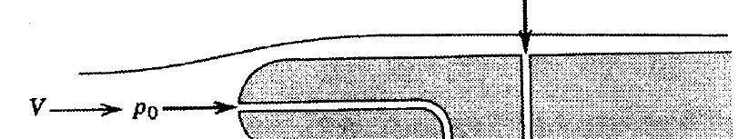
7 We can use the momentum theorem by itself to obtain useful results. In this example, we apply the momentum theorem to relate the force on a body to the properties p of the flow some distance from the body. This technique is useful in wind tunnel tests and is the basis of several fundamental theorems related to lift and induced drag of wings. We take the control volume shown below, bounded by the single surface, S which hwe divide id into 3 parts: the outer surface (S outer ), the inner surface (S inner ), and the pieces of the surface connecting the two (S*). We can write the integral form of the momentum equation for steady flow with no body forces as shown. 7
8 8
9 Note that the contribution from the part of the surface connecting S inner and S outer to the integrals is zero because as the two pieces of S* are made close together, th the unit normals point in opposite directions while p and V are equal. 9
10 Simplifying Approximations The equations of motion for a general fluid are extremely complex and even if the problem could be formulated it would be impractical to solve. Thus, from the outset, certain simplifying approximations that are often very accurate, are made. These may include the following assumptions. 10
11 Continuity and Homogeneity of the Fluid We assume that the fluid is composed of particles which are so small and plentiful l that t the statistically-averaged ti ti properties of interest are the same at any scale. This works well for gases and fluids under most conditions. It does not work for studying the flow of sand. It does not work when the fluid is so rarefied that the mean free path is of the same order as the dimensions of interest in the problem. The mean free path varies with altitude as shown in the next plot. Variation of temperature, pressure and density with altitude is also shown. We further assume that t the medium can be treated as a single type of fluid -- no suspensions of oil and water. 11
12 Variations of temperature, pressure and density with altitude. From: Kuethe &Ch Chow. 12
13 Variations of mean free path λ with altitude. From: Kuethe & Chow) 13
14 Inviscid idflow The effect of viscosity may sometimes be neglected or modelled indirectly. For many aerodynamic flows of interest, the region of high shear and vorticity is confined to a thin layer of fluid. Outside this layer, the fluid behaves as if it were inviscid. Thus the simpler equations of an inviscid fluid are often solved outside of the shear layers. There are some fluids which seem to be almost completely inviscid. Tests in superfluid helium have given results similar to inviscid calculations. 14
15 Incompressible (constant density) Flow PEMP When the fluid density does not change with changes in pressure, the fluid is incompressible. Water density changes very little with changes in pressure and is generally treated as an incompressible fluid. Air is compressible, but if pressure changes are small in comparison with some nominal value, the corresponding changes in density are small also and incompressible equations work quite well in describing the flow. The degree to which the fluid density changes with pressure is related to the speed of sound in the fluid. Thus, assuming that the flow is incompressible is equivalent to assuming that the speed of sound is infinite. When the local Mach number is less than 0.2 to 0.5 compressibility effects can often be ignored. The reason for this is discussed further in the chapter on compressibility, but one can see qualitatively that in order to make an appreciable change to the nominal 1 bar air pressure at sea level, substantial speeds are required. 15
16 Irrotational Flow Circulation is defined as: PEMP It is a measure of the rotation of an area of fluid. As the integration contour is shrunk down to a point, the ratio of circulation to the area enclosed by the curve is called the vorticity. Fluid that t starts t out without t rotational ti motion will not develop it unless there has been some shear stress acting on it. Some important exceptions to the idea that without viscosity irrotational flow remains irrotational: Vorticity can be created in a gravitational field when density gradients exist or in a rotating system (such as the earth) due to Coriolis forces. These are important sources of vorticity in meteorology. 16
17 And if the shear is confined to a small region, the vorticity it will be also. Thus, for many cases, especially in inviscid flow, much of the flow field may be treated as irrotational: curl V = 0 When this is the case, the vector field, V, may be written as the gradient of a scalar field, φ: V = grad φ where φ is the called the potential. This simplifies many of the equations discussed in subsequent sections. The velocity components are then: u = d φ / dx and v = d φ/ dy 17
18 Steady Flow When the variables describing the fluid properties p at a given point do not change in time, the flow may be treated as steady and the time derivatives in the equations of motion are zero. This condition depends on the chosen coordinate system. If the system is at rest with respect to a body in uniform motion through a fluid the equations in that system are steady, but expressed in a system fixed with respect to the undisturbed fluid, the flow is unsteady. It is often convenient to transform the coordinate system to one in which the flow is steady. This is, of course, not always possible. We will assume that the flow is steady in most of the discussions in this course but unsteady effects are often important in the study of bird flight, propellers, aircraft gust response, dynamics, and aeroelasticity as well as in the study of turbulence. We will always apply the first of these assumptions and will sometimes adopt one or more of the latter in the following discussions. 18
19 Equations of Fluid Flow The conservation laws may be used to derive the equations of fluid flow. These are supplemented with constitutive relations such as the perfect gas law: p = ρ R T or the isentropic relation between pressure and density: p /p = γ 2 1 (ρ 2 / ρ 1 ) We start with the Navier-Stokes equations and show how non- dimensionalising these equations leads to the non-dimensional parameters like Re and M. We then identify some of the most commonly-solved equations along with the corresponding assumptions. 19
20 The Navier-Stokes Equations The Navier-Stokes equations describe the flow of a continuous, Newtonian fluid. They may be derived from the principal of conservation of momentum applied for a field for an identified fluid particle. Hence we use the substantial derivative D( ) / Dt given by D( ) Dt ( ) ( ) ( ) ( ) ( ) r = + u + v + w = + V. ( t x y z t (For more details see Kuethe and Chow Appendix B, or, Moran Ch. 6, or, Anderson Ch. 15). ) 20
21 Here X, Y, Z are the body forces per unit mass in each direction and Tau is the stress tensor. X,Y, and Z are often associated with gravitational forces and are often neglected. ec ed. 21
22 The equations contain unknown stress terms τ xy and hence cannot be solved (not closed). They can be closed when the stress tensor is expressed in terms of viscosity, pressure and velocity (derivatives). Then the N-S equations simplify. 22
23 The stress at a point PEMP τ xy is the stress acting on the x-plane in the y-direction. Pressure is a normal compressive stress. μ (shear viscosity relating stresses to rate of strain) and λ (bulk viscosity relating stresses to div V) are the two viscosity coefficients. ). If pressure is a function only of density and not of the rate of change of density, then: λ = - (2/3)μ. Normal stresses: 23
24 See that now pressure in a moving fluid is the average of three normal stresses. Shear stresses depend only on μ : 24
25 S T i N i fl id Stress Tensor in a Newtonian fluid + = = + = u v u V μ σ σ μ λ σ ; 2 ) ( r + = = + = + = = + = w u v V y x x V yx xy xx μ σ σ μ λ σ μ σ σ μ λ σ ; 2 ). ( ; 2 ). ( r + = = + = + + w v w V x z y V zy yz zz zx xz yy μ σ σ μ λ σ μ σ σ μ λ σ ; 2 ). ( ; 2 ). ( r y z z zy yz zz μ μ ; ) ( 25
26 The Navier-Stokes equations for an incompressible fluid simplify to And the continuity equation for the incompressible flow (unsteady also) is u v w + + = 0 x y z 26
27 The Navier-Stokes equations in cylindrical coordinates (r, θ, z) are: 27
28 The Role of Non-Dimensional Equations PEMP The order of terms in the equations can be conveniently estimated by non-dimensionalising the equations. The procedure is demonstrated with simple incompressible equations. In the energy equation Φ is the viscous dissipation function. We start with the dimensional equations: 28
29 The equations are non-dimensionalised by non- dimensionalising i i independent d and dependent d variables through characteristic variables like V, L, ρ 1, a 1, T 1 etc. Here subscript 1 indicates some reference undisturbed flow conditions like at infinity. The new variables indicated by a prime are nondimensional. PEMP 29
30 Non-Dimensional Equations PEMP See how Reynolds number, Mach number and Prandtl number originate in the equations. It is clear from the momentum equation, for example, that when Re increases, the relative magnitude of the viscous term decreases. It is possible to infer this now since all the terms are scaled and it is possible to estimate. For details see Kuethe & Chow (Appendix B). Note ( Φ / μ 1 ) is non-d in this notation. 30
31 Solutions of the full Navier-Stokes equations show the onset of turbulence, the interaction of shear layers, and almost all of the interesting aerodynamic phenomena (with the exception of interacting or rarefied gas flows). Unfortunately, the equations are very difficult to solve. As the Reynolds number is increased, the scale of the interesting dynamics gets smaller so that most solutions of the full N-S equations are done at Reynolds numbers of 1 to 10,000 and for simple geometries. One of the most recent solutions of a flat plate boundary layer pushed the calculations to a Reynolds number of 1410 based on boundary layer thickness. These calculations took hundreds of hours on the Cray computer at NASA Ames. 31
32 Even at very small Reynolds numbers, the geometries which can be analyzed using the full N-S equations are quite simple and it currently does not make sense to consider solving these equations for realistic aircraft configurations. One reason that this is the case is that many of the approximate equations work quite well in such cases and are much more easily solved. 32
33 When the time averaged Navier-Stokes equations are not a sufficient description of the problem, one may resort to "large eddy simulations". This is a numerical solution of the time-dependent Navier-Stokes equations, with only the smaller scales of turbulence modeled in an averaged way. Larger scale turbulent motion can be included in this way. While this is faster than solving the full equations, it is still very slow. The figure below shows results from a large eddy simulation of the flow over a 2D circular cylinder. Each simulation required approximately 300 CPU hours and about 10 megawords of core memory on the Cray C-90. Figure from NASA / Parviz Moin. 33
34 Flow around a Cylinder simulated using Large Eddy Simulation (LES). From: NASA 34
35 Reynolds Averaged dnavier-stokes Equations One of the most popular pp simplifications made to the Navier- Stokes Equations is "Reynolds Averaging". This simplification to the full Navier-Stokes equations involves taking time averages of the velocity terms in the equations. Writing: u = <u> + u ', v = <v> + v', etc. (where < > represents a time average) with the fluctuations having zero mean value: <u'> = 0 we have: <u 2 > = <u> 2 + <u' 2 >, <uv> = <u><v> + <u'v'> 35
36 Reynolds Averaged dnavier-stokes Equations (Contd) This allows us to write the time-averaged NS equations as: and similarly for the y and z components. 36
37 Reynolds Averaged Navier-Stokes Equations (Contd) This looks just like the more general Navier Stokes equations for incompressible flow which hold for steady, laminar flow except that there are additional terms that act as additional stresses on the right hand side. These terms represent the effect of turbulence on the mean flow. They are called "Reynolds stresses" and are sometimes said to be caused by "eddy viscosity". These terms are generally much larger than the normal viscous terms. 37
38 The business of predicting these stresses and relating them to the computed mean flow properties is called turbulence modeling. This is usually accomplished empirically or by using the results of detailed timedependent simulations. Reynolds averaged NS solvers are appropriate for the analysis of viscous, compressible flows and have been applied to rather general configurations, i but one must be careful that the assumptions of the turbulence model are compatible with the characteristics of the flow of interest. 38


39 From NAS Technical Summaries, High-Lift Configuration CFD, Karlin Roth, NASA Ames Research Center 39
40 Euler Equations PEMP The momentum equation is sometimes called Euler's equation. (There are lots of equations called Euler equations!) But when people talk of solving the Euler equations these days, they are referring to the inviscid equations of motion given by: With some work*, the equation in the x direction becomes: or in vector notation: 40
41 These are combined with the equations of energy and continuity. The equations are often solved by finite differences whereby the values of each velocity component, the density, and the internal energy are computed at each point in the flow. From these quantities constitutive relations such as the perfect gas law or the isentropic pressure relation are used to find pressure. Since Euler equations permit rotational lflow and enthalpy losses (through shock waves), they are very useful in solving transonic flow problems, propeller or rotor aerodynamics, and flows with vortical structures in the field. 41
42 Mach number (Velocity magnitude?) contours by Euler equations. NOTE: Surface velocity is not zero. 42
43 Full Potential Equation The full potential equation is derived from the assumption of irrotational flow and the equations of continuity and momentum. The pressure and density terms in the Euler equations can be combined when use is made of the perfect gas law and the isentropic relation between pressure and density. Ashley and Landahl show how we may derive the following vector form of the unsteady full potential equation: 43
44 Full Potential Equation (Contd) This may be simplified for the case of steady flow in 2-D to: About the notation: When flow is irrotational curl V = 0 and by definition of curl and gradient: curl (grad φ) = 0 where φ is a scalar field. 44
45 Full Potential Equation (Contd) Thus we can define a nonphysical scalar potential, φ, that describes the velocity field. φ is related to the velocities by the relation: V = grad φ The equations can thus be written in terms of the unknown scalar rather than the 3 components of the velocity. This simplifies their solution. In the above expressions: a is the local speed of sound, x is the streamwise coordinate, and V is the vector velocity. Subscripts denote partial derivatives with respect to the subscripted variables (e.g. U x = du/dx) 45
 from TRANAIR analysis")


46 Mach contours (yellow = high; dark green = low) from TRANAIR analysis of a at Mach From NAS Technical Summaries 1994, Multipoint Aerodynamic Design, Forrester T. Johnson, Boeing Commercial lairplane Group. 46
47 Transonic Small Disturbance Equation When the full potential equation is simplified by assuming that perturbation velocities are small and we relate the local speed of sound dto the freestream value by making use of fthe isentropic i relations we obtain the small disturbance equation When we let the freestream Mach number go to one and ignore the last term, the equation becomes the classic transonic small disturbance equation: A great deal has been written about this nonlinear equation and its variants. (See Nixon.) It is used less frequently these days since finite difference methods can be used to solve the full potential equation directly.. 47
48 Prandtl-Glauert Equation The Prandtl-Glauert equation is a linearized form of the full potential equation. PEMP Full potential: If the velocity perturbations are much smaller than the freestream velocity, this expression becomes: or in the unsteady case: The 3-D version is easily constructed with the addition of z derivatives corresponding to the y derivatives shown here. 48
49 Note that this linearized form of the equation does not hold near the nose of an airfoil where the velocity perturbation is of the same order as the freestream, unless the freestream Mach number is itself small. Also note that t this expression holds for subsonic and supersonic flow (but not transonic flow). It forms the basis for many aerodynamic analysis methods. Analysis of P51 Mustang from Analytical Methods, Inc. using VSAERO, a code that solves the Prandtl-Glauert equations. 49
50 Acoustic Equation The acoustic equation may be obtained from the full potential equation by assuming that there is no freestream velocity, and that all perturbation velocities are small. PEMP Or, by changing from a coordinate system fixed to the body to one fixed with respect to the undisturbed fluid, the Prandtl- Glauert equation may be transformed to the acoustic equation. This equation is often used in the study of sound propagation and sometimes for rotor aerodynamics; thus the name. 50
51 Laplace's Equation Laplace's equation is the Prandtl-Glauert equation in the limit as the freestream Mach number goes to zero. It was actually first derived by Euler. The derivation is very simple, requiring only the equation of continuity, and the assumptions of irrotational and constant density flow. The continuity equation becomes then: Since the flow is irrotational: Substitution into the continuity equation yields: 51
52 Laplace's Equation (Contd) It is interesting to note that Laplace's equation does not require the assumption of small perturbations, while the Prandtl- Glauert equation does. In fact, near the stagnation point of an airfoil where velocities become small, the full potential equation reduces to Laplace's equation, not the Prandtl-Glauert equation. Note also that all of the time dependent terms in the full potential equation are multiplied by 1/a 2 so that this form of the equation holds for unsteady phenomena as well. 52
53 Bernoulli Equations Some of the equations we have discussed are posed in terms of state variables that do not include pressures. In these cases (e.g. the potential flow equations) the differential equations and boundary conditions allow one to compute the local velocities, but not the pressures. Once the velocities i are known, however, the momentum equation can be used to find the local pressure. Such equations are known as Bernoulli equations and they come in various forms, depending on the assumptions that can be made about the flow. 53
54 Bernoulli Equations (Contd) The conservation of momentum principle p is the source of the relation between pressure and velocity. It can be used very simply to derive the Bernoulli equation. To illustrate the basic physics behind the Bernoulli equations, we can derive a simple form: that for steady, incompressible flow. In this case we show that along a streamline: 54
55 When the flow is not steady, the Euler equations can be integrated to obtain a more general form of this result: Kelvin's equation, the Bernoulli equation for irrotational flow. where f is a body force per unit mass (such as gravity) and F is an arbitrary function of time. 55
56 If we do not assume that the flow is irrotational, we cannot introduce the potential and the expression is not so nicely integrable. If, however, we assume that the flow is steady with no "body forces", but not necessarily irrotational we can write the following expression that holds along a streamline: While the above equations hold for steady flows along a streamline, for irrotational flows they hold throughout the fluid. 56
57 We can derive a more useful form of the Bernoulli equation by starting with the expression for steady flow without body forces shown just above. If the flow is assumed to be isentropic flow (no entropy change or heat addition): p = constant * ρ γ Substitution yields the compressible Bernoulli equation: This actually works for adiabatic flows as well as isentropic flows. 57
58 In summary, we often deal with one of two simple forms of the Bernoulli equation shown below. 58
59 The Pressures In both the incompressible and compressible forms of Bernoulli's equation shown above there are 3 terms. The quantity p T is the total or stagnation pressure. It is the pressure that would be measured at points in the flow where V = 0. The other p in the above expressions is the static pressure. Note that in incompressible flow, the speed is directly related to the difference in total and static pressure. This can be measured directly with a pitot-static probe shown below. 59

60 The Pitot-Static Probe PEMP The Ventui Tube 60
61 The dynamic pressure is defined as: The static pressure coefficient is defined as: where p is the freestream static pressure. In incompressible flow, the expression for C p is especially simple: If the local velocity is expressed as a small perturbation in the freestream: Then the incompressible C p relation can be written: 61
62 The expression for C p in compressible isentropic flow (sometimes called the isentropic pressure rule) is derived from the compressible Bernoulli equation along with the expression for the speed of sound in a perfect gas. In terms of the local Mach number the expression is: 62
63 We can tell if the flow is supersonic, just by looking at the value of C p. The critical value of C p, denoted C p * is found by setting M = 1 in the above expression (for gamma = 1.4): Also, we see that there is a minimum value of C p, corresponding to a complete vacuum. Setting the local Mach number to infinity yields: C p cannot be any more negative than this. Experiments show that airfoils can get to about 70% of vacuum C p. This can limit the maximum lift of supersonic wings. 63
64 Simple Bernoulli Derivation The momentum equation for this flow can be written in terms of the flow through h a small control volume. The change in momentum per unit time is: ρ S V (V+dV) - ρ S V 2 = ρ S V dv This change in momentum arises from the pressures acting along the faces of the control volume: pressure force (ends) = ps - (p+dp)(s+ds) = -p ds - S dp pressure force (sides) = (p + dp/2) ds = p ds (to first order) pressure (total) = -S dp 64
65 Simple Bernoulli Derivation (Contd) Equating the force due to pressure with the force required to produce the momentum change yields: -S dp = ρ S V dv or dp = -ρ V dv This is a simple form of the Euler equation. In the case that ρ = constant, the above equation may be integrated to produce the incompressible form of the Bernoulli equation: p 2 + ρ/2 V 22 = p 1 + ρ/2 V 2 1 or: p + ρ/2 V 2 = p t 65
66 Summary The following topics were dealt in this session Conservation laws Different simplifying approximations and the resulting equations The role of non-dimensional equations Bernoulli s equation and eh pressure distribution 66
67 Thank you 67
CHAPTER 7 SEVERAL FORMS OF THE EQUATIONS OF MOTION
 CHAPTER 7 SEVERAL FORMS OF THE EQUATIONS OF MOTION 7.1 THE NAVIER-STOKES EQUATIONS Under the assumption of a Newtonian stress-rate-of-strain constitutive equation and a linear, thermally conductive medium,
Introduction to Aerodynamics. Dr. Guven Aerospace Engineer (P.hD)
") Introduction to Aerodynamics Dr. Guven Aerospace Engineer (P.hD) Aerodynamic Forces All aerodynamic forces are generated wither through pressure distribution or a shear stress distribution on a body. The
Introduction to Aerodynamics Dr. Guven Aerospace Engineer (P.hD) Aerodynamic Forces All aerodynamic forces are generated wither through pressure distribution or a shear stress distribution on a body. The
Aerodynamics. Lecture 1: Introduction - Equations of Motion G. Dimitriadis
 Aerodynamics Lecture 1: Introduction - Equations of Motion G. Dimitriadis Definition Aerodynamics is the science that analyses the flow of air around solid bodies The basis of aerodynamics is fluid dynamics
Fundamentals of Aerodynamics
 Fundamentals of Aerodynamics Fourth Edition John D. Anderson, Jr. Curator of Aerodynamics National Air and Space Museum Smithsonian Institution and Professor Emeritus University of Maryland Me Graw Hill
PEMP ACD2505. M.S. Ramaiah School of Advanced Studies, Bengaluru
 Two-Dimensional Potential Flow Session delivered by: Prof. M. D. Deshpande 1 Session Objectives -- At the end of this session the delegate would have understood PEMP The potential theory and its application
Compressible Potential Flow: The Full Potential Equation. Copyright 2009 Narayanan Komerath
 Compressible Potential Flow: The Full Potential Equation 1 Introduction Recall that for incompressible flow conditions, velocity is not large enough to cause density changes, so density is known. Thus
V (r,t) = i ˆ u( x, y,z,t) + ˆ j v( x, y,z,t) + k ˆ w( x, y, z,t)
 = i ˆ u( x, y,z,t) + ˆ j v( x, y,z,t) + k ˆ w( x, y, z,t)") IV. DIFFERENTIAL RELATIONS FOR A FLUID PARTICLE This chapter presents the development and application of the basic differential equations of fluid motion. Simplifications in the general equations and common
IV. DIFFERENTIAL RELATIONS FOR A FLUID PARTICLE This chapter presents the development and application of the basic differential equations of fluid motion. Simplifications in the general equations and common
Chapter 5. The Differential Forms of the Fundamental Laws
 Chapter 5 The Differential Forms of the Fundamental Laws 1 5.1 Introduction Two primary methods in deriving the differential forms of fundamental laws: Gauss s Theorem: Allows area integrals of the equations
Fundamentals of Aerodynamits
 Fundamentals of Aerodynamits Fifth Edition in SI Units John D. Anderson, Jr. Curator of Aerodynamics National Air and Space Museum Smithsonian Institution and Professor Emeritus University of Maryland
High Speed Aerodynamics. Copyright 2009 Narayanan Komerath
 Welcome to High Speed Aerodynamics 1 Lift, drag and pitching moment? Linearized Potential Flow Transformations Compressible Boundary Layer WHAT IS HIGH SPEED AERODYNAMICS? Airfoil section? Thin airfoil
Detailed Outline, M E 320 Fluid Flow, Spring Semester 2015
 Detailed Outline, M E 320 Fluid Flow, Spring Semester 2015 I. Introduction (Chapters 1 and 2) A. What is Fluid Mechanics? 1. What is a fluid? 2. What is mechanics? B. Classification of Fluid Flows 1. Viscous
Chapter 9: Differential Analysis
 9-1 Introduction 9-2 Conservation of Mass 9-3 The Stream Function 9-4 Conservation of Linear Momentum 9-5 Navier Stokes Equation 9-6 Differential Analysis Problems Recall 9-1 Introduction (1) Chap 5: Control
2. Getting Ready for Computational Aerodynamics: Fluid Mechanics Foundations
 . Getting Ready for Computational Aerodynamics: Fluid Mechanics Foundations We need to review the governing equations of fluid mechanics before examining the methods of computational aerodynamics in detail.
Continuum Mechanics Lecture 5 Ideal fluids
 Continuum Mechanics Lecture 5 Ideal fluids Prof. http://www.itp.uzh.ch/~teyssier Outline - Helmholtz decomposition - Divergence and curl theorem - Kelvin s circulation theorem - The vorticity equation
Detailed Outline, M E 521: Foundations of Fluid Mechanics I
 Detailed Outline, M E 521: Foundations of Fluid Mechanics I I. Introduction and Review A. Notation 1. Vectors 2. Second-order tensors 3. Volume vs. velocity 4. Del operator B. Chapter 1: Review of Basic
Thin airfoil theory. Chapter Compressible potential flow The full potential equation
 hapter 4 Thin airfoil theory 4. ompressible potential flow 4.. The full potential equation In compressible flow, both the lift and drag of a thin airfoil can be determined to a reasonable level of accuracy
FUNDAMENTALS OF AERODYNAMICS
 *A \ FUNDAMENTALS OF AERODYNAMICS Second Edition John D. Anderson, Jr. Professor of Aerospace Engineering University of Maryland H ' McGraw-Hill, Inc. New York St. Louis San Francisco Auckland Bogota Caracas
Chapter 9: Differential Analysis of Fluid Flow
 of Fluid Flow Objectives 1. Understand how the differential equations of mass and momentum conservation are derived. 2. Calculate the stream function and pressure field, and plot streamlines for a known
SPC Aerodynamics Course Assignment Due Date Monday 28 May 2018 at 11:30
 SPC 307 - Aerodynamics Course Assignment Due Date Monday 28 May 2018 at 11:30 1. The maximum velocity at which an aircraft can cruise occurs when the thrust available with the engines operating with the
Notes 4: Differential Form of the Conservation Equations
 Low Speed Aerodynamics Notes 4: Differential Form of the Conservation Equations Deriving Conservation Equations From the Laws of Physics Physical Laws Fluids, being matter, must obey the laws of Physics.
6.1 Momentum Equation for Frictionless Flow: Euler s Equation The equations of motion for frictionless flow, called Euler s
 Chapter 6 INCOMPRESSIBLE INVISCID FLOW All real fluids possess viscosity. However in many flow cases it is reasonable to neglect the effects of viscosity. It is useful to investigate the dynamics of an
Several forms of the equations of motion
 Chapter 6 Several forms of the equations of motion 6.1 The Navier-Stokes equations Under the assumption of a Newtonian stress-rate-of-strain constitutive equation and a linear, thermally conductive medium,
Introduction to Aerospace Engineering
 Introduction to Aerospace Engineering Lecture slides Challenge the future 3-0-0 Introduction to Aerospace Engineering Aerodynamics 5 & 6 Prof. H. Bijl ir. N. Timmer Delft University of Technology 5. Compressibility
Aerodynamics. Basic Aerodynamics. Continuity equation (mass conserved) Some thermodynamics. Energy equation (energy conserved)
 Some thermodynamics. Energy equation (energy conserved)") Flow with no friction (inviscid) Aerodynamics Basic Aerodynamics Continuity equation (mass conserved) Flow with friction (viscous) Momentum equation (F = ma) 1. Euler s equation 2. Bernoulli s equation
Flow with no friction (inviscid) Aerodynamics Basic Aerodynamics Continuity equation (mass conserved) Flow with friction (viscous) Momentum equation (F = ma) 1. Euler s equation 2. Bernoulli s equation
In this section, mathematical description of the motion of fluid elements moving in a flow field is
 Jun. 05, 015 Chapter 6. Differential Analysis of Fluid Flow 6.1 Fluid Element Kinematics In this section, mathematical description of the motion of fluid elements moving in a flow field is given. A small
for what specific application did Henri Pitot develop the Pitot tube? what was the name of NACA s (now NASA) first research laboratory?
 first research laboratory?") 1. 5% short answers for what specific application did Henri Pitot develop the Pitot tube? what was the name of NACA s (now NASA) first research laboratory? in what country (per Anderson) was the first
1. 5% short answers for what specific application did Henri Pitot develop the Pitot tube? what was the name of NACA s (now NASA) first research laboratory? in what country (per Anderson) was the first
Continuity Equation for Compressible Flow
 Continuity Equation for Compressible Flow Velocity potential irrotational steady compressible Momentum (Euler) Equation for Compressible Flow Euler's equation isentropic velocity potential equation for
Numerical Heat and Mass Transfer
 Master Degree in Mechanical Engineering Numerical Heat and Mass Transfer 15-Convective Heat Transfer Fausto Arpino f.arpino@unicas.it Introduction In conduction problems the convection entered the analysis
To study the motion of a perfect gas, the conservation equations of continuity
 Chapter 1 Ideal Gas Flow The Navier-Stokes equations To study the motion of a perfect gas, the conservation equations of continuity ρ + (ρ v = 0, (1.1 momentum ρ D v Dt = p+ τ +ρ f m, (1.2 and energy ρ
AA214B: NUMERICAL METHODS FOR COMPRESSIBLE FLOWS
 AA214B: NUMERICAL METHODS FOR COMPRESSIBLE FLOWS 1 / 29 AA214B: NUMERICAL METHODS FOR COMPRESSIBLE FLOWS Hierarchy of Mathematical Models 1 / 29 AA214B: NUMERICAL METHODS FOR COMPRESSIBLE FLOWS 2 / 29
Chapter 6: Incompressible Inviscid Flow
 Chapter 6: Incompressible Inviscid Flow 6-1 Introduction 6-2 Nondimensionalization of the NSE 6-3 Creeping Flow 6-4 Inviscid Regions of Flow 6-5 Irrotational Flow Approximation 6-6 Elementary Planar Irrotational
Introduction to Fluid Mechanics
 Introduction to Fluid Mechanics Tien-Tsan Shieh April 16, 2009 What is a Fluid? The key distinction between a fluid and a solid lies in the mode of resistance to change of shape. The fluid, unlike the
Given the water behaves as shown above, which direction will the cylinder rotate?
 water stream fixed but free to rotate Given the water behaves as shown above, which direction will the cylinder rotate? ) Clockwise 2) Counter-clockwise 3) Not enough information F y U 0 U F x V=0 V=0
Steady waves in compressible flow
 Chapter Steady waves in compressible flow. Oblique shock waves Figure. shows an oblique shock wave produced when a supersonic flow is deflected by an angle. Figure.: Flow geometry near a plane oblique
Introduction to Aerospace Engineering
 4. Basic Fluid (Aero) Dynamics Introduction to Aerospace Engineering Here, we will try and look at a few basic ideas from the complicated field of fluid dynamics. The general area includes studies of incompressible,
1. Introduction, tensors, kinematics
 1. Introduction, tensors, kinematics Content: Introduction to fluids, Cartesian tensors, vector algebra using tensor notation, operators in tensor form, Eulerian and Lagrangian description of scalar and
AA210A Fundamentals of Compressible Flow. Chapter 5 -The conservation equations
 AA210A Fundamentals of Compressible Flow Chapter 5 -The conservation equations 1 5.1 Leibniz rule for differentiation of integrals Differentiation under the integral sign. According to the fundamental
1. Introduction Some Basic Concepts
 1. Introduction Some Basic Concepts 1.What is a fluid? A substance that will go on deforming in the presence of a deforming force, however small 2. What Properties Do Fluids Have? Density ( ) Pressure
ACD2503 Aircraft Aerodynamics
 ACD2503 Aircraft Aerodynamics Session delivered by: Prof. M. D. Deshpande 1 Aims and Summary PEMP It is intended dto prepare students for participation i i in the design process of an aircraft and its
J. Szantyr Lecture No. 4 Principles of the Turbulent Flow Theory The phenomenon of two markedly different types of flow, namely laminar and
 J. Szantyr Lecture No. 4 Principles of the Turbulent Flow Theory The phenomenon of two markedly different types of flow, namely laminar and turbulent, was discovered by Osborne Reynolds (184 191) in 1883
Review of fluid dynamics
 Chapter 2 Review of fluid dynamics 2.1 Preliminaries ome basic concepts: A fluid is a substance that deforms continuously under stress. A Material olume is a tagged region that moves with the fluid. Hence
Chapter 4: Fluid Kinematics
 Overview Fluid kinematics deals with the motion of fluids without considering the forces and moments which create the motion. Items discussed in this Chapter. Material derivative and its relationship to
Copyright 2007 N. Komerath. Other rights may be specified with individual items. All rights reserved.
 Low Speed Aerodynamics Notes 5: Potential ti Flow Method Objective: Get a method to describe flow velocity fields and relate them to surface shapes consistently. Strategy: Describe the flow field as the
AE/ME 339. K. M. Isaac Professor of Aerospace Engineering. 12/21/01 topic7_ns_equations 1
 AE/ME 339 Professor of Aerospace Engineering 12/21/01 topic7_ns_equations 1 Continuity equation Governing equation summary Non-conservation form D Dt. V 0.(2.29) Conservation form ( V ) 0...(2.33) t 12/21/01
Fundamentals of Fluid Dynamics: Elementary Viscous Flow
 Fundamentals of Fluid Dynamics: Elementary Viscous Flow Introductory Course on Multiphysics Modelling TOMASZ G. ZIELIŃSKI bluebox.ippt.pan.pl/ tzielins/ Institute of Fundamental Technological Research
3. FORMS OF GOVERNING EQUATIONS IN CFD
 3. FORMS OF GOVERNING EQUATIONS IN CFD 3.1. Governing and model equations in CFD Fluid flows are governed by the Navier-Stokes equations (N-S), which simpler, inviscid, form is the Euler equations. For
BLUFF-BODY AERODYNAMICS
 International Advanced School on WIND-EXCITED AND AEROELASTIC VIBRATIONS OF STRUCTURES Genoa, Italy, June 12-16, 2000 BLUFF-BODY AERODYNAMICS Lecture Notes by Guido Buresti Department of Aerospace Engineering
Viscous flow along a wall
 Chapter 8 Viscous flow along a wall 8. The no-slip condition All liquids and gases are viscous and, as a consequence, a fluid near a solid boundary sticks to the boundary. The tendency for a liquid or
What we know about Fluid Mechanics. What we know about Fluid Mechanics
 What we know about Fluid Mechanics 1. Survey says. 3. Image from: www.axs.com 4. 5. 6. 1 What we know about Fluid Mechanics 1. MEB (single input, single output, steady, incompressible, no rxn, no phase
1. Fluid Dynamics Around Airfoils
 1. Fluid Dynamics Around Airfoils Two-dimensional flow around a streamlined shape Foces on an airfoil Distribution of pressue coefficient over an airfoil The variation of the lift coefficient with the
Inviscid & Incompressible flow
 < 3.1. Introduction and Road Map > Basic aspects of inviscid, incompressible flow Bernoulli s Equation Laplaces s Equation Some Elementary flows Some simple applications 1.Venturi 2. Low-speed wind tunnel
AE/ME 339. Computational Fluid Dynamics (CFD) K. M. Isaac. Momentum equation. Computational Fluid Dynamics (AE/ME 339) MAEEM Dept.
 K. M. Isaac. Momentum equation. Computational Fluid Dynamics (AE/ME 339) MAEEM Dept.") AE/ME 339 Computational Fluid Dynamics (CFD) 9//005 Topic7_NS_ F0 1 Momentum equation 9//005 Topic7_NS_ F0 1 Consider the moving fluid element model shown in Figure.b Basis is Newton s nd Law which says
AE/ME 339 Computational Fluid Dynamics (CFD) 9//005 Topic7_NS_ F0 1 Momentum equation 9//005 Topic7_NS_ F0 1 Consider the moving fluid element model shown in Figure.b Basis is Newton s nd Law which says
AOE 3114 Compressible Aerodynamics
 AOE 114 Compressible Aerodynamics Primary Learning Objectives The student will be able to: 1. Identify common situations in which compressibility becomes important in internal and external aerodynamics
Introduction and Basic Concepts
 Topic 1 Introduction and Basic Concepts 1 Flow Past a Circular Cylinder Re = 10,000 and Mach approximately zero Mach = 0.45 Mach = 0.64 Pictures are from An Album of Fluid Motion by Van Dyke Flow Past
EKC314: TRANSPORT PHENOMENA Core Course for B.Eng.(Chemical Engineering) Semester II (2008/2009)
 Semester II (2008/2009)") EKC314: TRANSPORT PHENOMENA Core Course for B.Eng.(Chemical Engineering) Semester II (2008/2009) Dr. Mohamad Hekarl Uzir-chhekarl@eng.usm.my School of Chemical Engineering Engineering Campus, Universiti
EKC314: TRANSPORT PHENOMENA Core Course for B.Eng.(Chemical Engineering) Semester II (2008/2009) Dr. Mohamad Hekarl Uzir-chhekarl@eng.usm.my School of Chemical Engineering Engineering Campus, Universiti
Fundamentals of Fluid Mechanics
 Sixth Edition Fundamentals of Fluid Mechanics International Student Version BRUCE R. MUNSON DONALD F. YOUNG Department of Aerospace Engineering and Engineering Mechanics THEODORE H. OKIISHI Department
Principles of Convection
 Principles of Convection Point Conduction & convection are similar both require the presence of a material medium. But convection requires the presence of fluid motion. Heat transfer through the: Solid
The conservation equations
 Chapter 5 The conservation equations 5.1 Leibniz rule for di erentiation of integrals 5.1.1 Di erentiation under the integral sign According to the fundamental theorem of calculus if f is a smooth function
AA210A Fundamentals of Compressible Flow. Chapter 1 - Introduction to fluid flow
 AA210A Fundamentals of Compressible Flow Chapter 1 - Introduction to fluid flow 1 1.2 Conservation of mass Mass flux in the x-direction [ ρu ] = M L 3 L T = M L 2 T Momentum per unit volume Mass per unit
FLUID MECHANICS. Chapter 9 Flow over Immersed Bodies
 FLUID MECHANICS Chapter 9 Flow over Immersed Bodies CHAP 9. FLOW OVER IMMERSED BODIES CONTENTS 9.1 General External Flow Characteristics 9.3 Drag 9.4 Lift 9.1 General External Flow Characteristics 9.1.1
Fundamentals of Fluid Dynamics: Ideal Flow Theory & Basic Aerodynamics
 Fundamentals of Fluid Dynamics: Ideal Flow Theory & Basic Aerodynamics Introductory Course on Multiphysics Modelling TOMASZ G. ZIELIŃSKI (after: D.J. ACHESON s Elementary Fluid Dynamics ) bluebox.ippt.pan.pl/
Introduction to Turbulence AEEM Why study turbulent flows?
 Introduction to Turbulence AEEM 7063-003 Dr. Peter J. Disimile UC-FEST Department of Aerospace Engineering Peter.disimile@uc.edu Intro to Turbulence: C1A Why 1 Most flows encountered in engineering and
Concept: AERODYNAMICS
 1 Concept: AERODYNAMICS 2 Narayanan Komerath 3 4 Keywords: Flow Potential Flow Lift, Drag, Dynamic Pressure, Irrotational, Mach Number, Reynolds Number, Incompressible 5 6 7 1. Definition When objects
Fluid Dynamics: Theory, Computation, and Numerical Simulation Second Edition
 Fluid Dynamics: Theory, Computation, and Numerical Simulation Second Edition C. Pozrikidis m Springer Contents Preface v 1 Introduction to Kinematics 1 1.1 Fluids and solids 1 1.2 Fluid parcels and flow
List of symbols. Latin symbols. Symbol Property Unit
 Abstract Aircraft icing continues to be a threat for modern day aircraft. Icing occurs when supercooled large droplets (SLD s) impinge on the body of the aircraft. These droplets can bounce off, freeze
Outlines. simple relations of fluid dynamics Boundary layer analysis. Important for basic understanding of convection heat transfer
 Forced Convection Outlines To examine the methods of calculating convection heat transfer (particularly, the ways of predicting the value of convection heat transfer coefficient, h) Convection heat transfer
AE 2020: Low Speed Aerodynamics. I. Introductory Remarks Read chapter 1 of Fundamentals of Aerodynamics by John D. Anderson
 AE 2020: Low Speed Aerodynamics I. Introductory Remarks Read chapter 1 of Fundamentals of Aerodynamics by John D. Anderson Text Book Anderson, Fundamentals of Aerodynamics, 4th Edition, McGraw-Hill, Inc.
Boundary-Layer Theory
 Hermann Schlichting Klaus Gersten Boundary-Layer Theory With contributions from Egon Krause and Herbert Oertel Jr. Translated by Katherine Mayes 8th Revised and Enlarged Edition With 287 Figures and 22
Chapter 1: Basic Concepts
 What is a fluid? A fluid is a substance in the gaseous or liquid form Distinction between solid and fluid? Solid: can resist an applied shear by deforming. Stress is proportional to strain Fluid: deforms
The E80 Wind Tunnel Experiment the experience will blow you away. by Professor Duron Spring 2012
 The E80 Wind Tunnel Experiment the experience will blow you away by Professor Duron Spring 2012 Objectives To familiarize the student with the basic operation and instrumentation of the HMC wind tunnel
Homework Two. Abstract: Liu. Solutions for Homework Problems Two: (50 points total). Collected by Junyu
. Collected by Junyu") Homework Two Abstract: Liu. Solutions for Homework Problems Two: (50 points total). Collected by Junyu Contents 1 BT Problem 13.15 (8 points) (by Nick Hunter-Jones) 1 2 BT Problem 14.2 (12 points: 3+3+3+3)
Homework Two Abstract: Liu. Solutions for Homework Problems Two: (50 points total). Collected by Junyu Contents 1 BT Problem 13.15 (8 points) (by Nick Hunter-Jones) 1 2 BT Problem 14.2 (12 points: 3+3+3+3)
Review of Fluid Mechanics
 Chapter 3 Review of Fluid Mechanics 3.1 Units and Basic Definitions Newton s Second law forms the basis of all units of measurement. For a particle of mass m subjected to a resultant force F the law may
Contents. I Introduction 1. Preface. xiii
 Contents Preface xiii I Introduction 1 1 Continuous matter 3 1.1 Molecules................................ 4 1.2 The continuum approximation.................... 6 1.3 Newtonian mechanics.........................
Supersonic Aerodynamics. Methods and Applications
 Supersonic Aerodynamics Methods and Applications Outline Introduction to Supersonic Flow Governing Equations Numerical Methods Aerodynamic Design Applications Introduction to Supersonic Flow What does
the pitot static measurement equal to a constant C which is to take into account the effect of viscosity and so on.
 Mechanical Measurements and Metrology Prof. S. P. Venkateshan Department of Mechanical Engineering Indian Institute of Technology, Madras Module -2 Lecture - 27 Measurement of Fluid Velocity We have been
Quick Recapitulation of Fluid Mechanics
 Quick Recapitulation of Fluid Mechanics Amey Joshi 07-Feb-018 1 Equations of ideal fluids onsider a volume element of a fluid of density ρ. If there are no sources or sinks in, the mass in it will change
A Study on Numerical Solution to the Incompressible Navier-Stokes Equation
 A Study on Numerical Solution to the Incompressible Navier-Stokes Equation Zipeng Zhao May 2014 1 Introduction 1.1 Motivation One of the most important applications of finite differences lies in the field
A Study of Transonic Flow and Airfoils. Presented by: Huiliang Lui 30 th April 2007
 A Study of Transonic Flow and Airfoils Presented by: Huiliang Lui 3 th April 7 Contents Background Aims Theory Conservation Laws Irrotational Flow Self-Similarity Characteristics Numerical Modeling Conclusion
Fundamentals of Fluid Dynamics: Waves in Fluids
 Fundamentals of Fluid Dynamics: Waves in Fluids Introductory Course on Multiphysics Modelling TOMASZ G. ZIELIŃSKI (after: D.J. ACHESON s Elementary Fluid Dynamics ) bluebox.ippt.pan.pl/ tzielins/ Institute
Given a stream function for a cylinder in a uniform flow with circulation: a) Sketch the flow pattern in terms of streamlines.
 Sketch the flow pattern in terms of streamlines.") Question Given a stream function for a cylinder in a uniform flow with circulation: R Γ r ψ = U r sinθ + ln r π R a) Sketch the flow pattern in terms of streamlines. b) Derive an expression for the angular
Question Given a stream function for a cylinder in a uniform flow with circulation: R Γ r ψ = U r sinθ + ln r π R a) Sketch the flow pattern in terms of streamlines. b) Derive an expression for the angular
AE301 Aerodynamics I UNIT B: Theory of Aerodynamics
 AE301 Aerodynamics I UNIT B: Theory of Aerodynamics ROAD MAP... B-1: Mathematics for Aerodynamics B-: Flow Field Representations B-3: Potential Flow Analysis B-4: Applications of Potential Flow Analysis
FLUID MECHANICS. Atmosphere, Ocean. Aerodynamics. Energy conversion. Transport of heat/other. Numerous industrial processes
 SG2214 Anders Dahlkild Luca Brandt FLUID MECHANICS : SG2214 Course requirements (7.5 cr.) INL 1 (3 cr.) 3 sets of home work problems (for 10 p. on written exam) 1 laboration TEN1 (4.5 cr.) 1 written exam
4 Compressible Fluid Dynamics
 4 Compressible Fluid Dynamics 4. Compressible flow definitions Compressible flow describes the behaviour of fluids that experience significant variations in density under the application of external pressures.
Masters in Mechanical Engineering. Problems of incompressible viscous flow. 2µ dx y(y h)+ U h y 0 < y < h,
+ U h y 0 < y < h,") Masters in Mechanical Engineering Problems of incompressible viscous flow 1. Consider the laminar Couette flow between two infinite flat plates (lower plate (y = 0) with no velocity and top plate (y =
Masters in Mechanical Engineering Problems of incompressible viscous flow 1. Consider the laminar Couette flow between two infinite flat plates (lower plate (y = 0) with no velocity and top plate (y =
Chapter 1 Fluid Characteristics
 Chapter 1 Fluid Characteristics 1.1 Introduction 1.1.1 Phases Solid increasing increasing spacing and intermolecular liquid latitude of cohesive Fluid gas (vapor) molecular force plasma motion 1.1.2 Fluidity
Flight Vehicle Terminology
 Flight Vehicle Terminology 1.0 Axes Systems There are 3 axes systems which can be used in Aeronautics, Aerodynamics & Flight Mechanics: Ground Axes G(x 0, y 0, z 0 ) Body Axes G(x, y, z) Aerodynamic Axes
Syllabus for AE3610, Aerodynamics I
 Syllabus for AE3610, Aerodynamics I Current Catalog Data: AE 3610 Aerodynamics I Credit: 4 hours A study of incompressible aerodynamics of flight vehicles with emphasis on combined application of theory
Iran University of Science & Technology School of Mechanical Engineering Advance Fluid Mechanics
 1. Consider a sphere of radius R immersed in a uniform stream U0, as shown in 3 R Fig.1. The fluid velocity along streamline AB is given by V ui U i x 1. 0 3 Find (a) the position of maximum fluid acceleration
Lecture Notes Fluid Mechanics of Turbomachines II
 Lecture Notes Fluid Mechanics of Turbomachines II N.P. Kruyt 999-2009 N.P. Kruyt Turbomachinery Laboratory Engineering Fluid Dynamics Department of Mechanical Engineering University of Twente The Netherlands
Part A: 1 pts each, 10 pts total, no partial credit.
 Part A: 1 pts each, 10 pts total, no partial credit. 1) (Correct: 1 pt/ Wrong: -3 pts). The sum of static, dynamic, and hydrostatic pressures is constant when flow is steady, irrotational, incompressible,
Fluid Mechanics Prof. T.I. Eldho Department of Civil Engineering Indian Institute of Technology, Bombay. Lecture - 17 Laminar and Turbulent flows
 Fluid Mechanics Prof. T.I. Eldho Department of Civil Engineering Indian Institute of Technology, Bombay Lecture - 17 Laminar and Turbulent flows Welcome back to the video course on fluid mechanics. In
Chapter 1. Governing Equations of GFD. 1.1 Mass continuity
 Chapter 1 Governing Equations of GFD The fluid dynamical governing equations consist of an equation for mass continuity, one for the momentum budget, and one or more additional equations to account for
William В. Brower, Jr. A PRIMER IN FLUID MECHANICS. Dynamics of Flows in One Space Dimension. CRC Press Boca Raton London New York Washington, D.C.
 William В. Brower, Jr. A PRIMER IN FLUID MECHANICS Dynamics of Flows in One Space Dimension CRC Press Boca Raton London New York Washington, D.C. Table of Contents Chapter 1 Fluid Properties Kinetic Theory
In which of the following scenarios is applying the following form of Bernoulli s equation: steady, inviscid, uniform stream of water. Ma = 0.
 bernoulli_11 In which of the following scenarios is applying the following form of Bernoulli s equation: p V z constant! g + g + = from point 1 to point valid? a. 1 stagnant column of water steady, inviscid,
Chapter 2: Basic Governing Equations
 -1 Reynolds Transport Theorem (RTT) - Continuity Equation -3 The Linear Momentum Equation -4 The First Law of Thermodynamics -5 General Equation in Conservative Form -6 General Equation in Non-Conservative
PART 1B EXPERIMENTAL ENGINEERING. SUBJECT: FLUID MECHANICS & HEAT TRANSFER LOCATION: HYDRAULICS LAB (Gnd Floor Inglis Bldg) BOUNDARY LAYERS AND DRAG
 BOUNDARY LAYERS AND DRAG") 1 PART 1B EXPERIMENTAL ENGINEERING SUBJECT: FLUID MECHANICS & HEAT TRANSFER LOCATION: HYDRAULICS LAB (Gnd Floor Inglis Bldg) EXPERIMENT T3 (LONG) BOUNDARY LAYERS AND DRAG OBJECTIVES a) To measure the velocity
1 PART 1B EXPERIMENTAL ENGINEERING SUBJECT: FLUID MECHANICS & HEAT TRANSFER LOCATION: HYDRAULICS LAB (Gnd Floor Inglis Bldg) EXPERIMENT T3 (LONG) BOUNDARY LAYERS AND DRAG OBJECTIVES a) To measure the velocity
Introduction to Flight
 l_ Introduction to Flight Fifth Edition John D. Anderson, Jr. Curator for Aerodynamics, National Air and Space Museum Smithsonian Institution Professor Emeritus University of Maryland Me Graw Higher Education
Entropy generation and transport
 Chapter 7 Entropy generation and transport 7.1 Convective form of the Gibbs equation In this chapter we will address two questions. 1) How is Gibbs equation related to the energy conservation equation?
NDT&E Methods: UT. VJ Technologies CAVITY INSPECTION. Nondestructive Testing & Evaluation TPU Lecture Course 2015/16.
 CAVITY INSPECTION NDT&E Methods: UT VJ Technologies NDT&E Methods: UT 6. NDT&E: Introduction to Methods 6.1. Ultrasonic Testing: Basics of Elasto-Dynamics 6.2. Principles of Measurement 6.3. The Pulse-Echo
Compressible Fluid Flow
 Compressible Fluid Flow For B.E/B.Tech Engineering Students As Per Revised Syllabus of Leading Universities in India Including Dr. APJ Abdul Kalam Technological University, Kerala Dr. S. Ramachandran,