Reference : McCabe, W.L. Smith J.C. & Harriett P., Unit Operations of Chemical

Transcription

1 1

2 Course materials (References) Textbook: Welty J. R., Wicks, C. E., Wilson, R. E., & Rorrer, G., Fundamentals of Momentum Heat, and Mass Transfer, 4th Edition, John Wiley & Sons.2000 Reference : McCabe, W.L. Smith J.C. & Harriett P., Unit Operations of Chemical Engineering, 5th Edition. McGraw Hill, 1993 Course Contents: The following topics will be covered in the formal lectures: NO Topic Covered During Class Duration in Weeks 1 Fluid and Flow properties 1 2 Conservation of mass 2 3 Newton s second law of motion 1 4 Conservation of energy 2 5 Shear stress in laminar flow 1 6 Analysis of a differential fluid element in laminar flow 1 7 Differential equations of fluid flow 1 8 Dimensional analysis 1 9 Viscous flow and the boundary layer concept 1 Course objectives: The objectives of this course are to: 1. know how to solve basic fluid statics problems 2. know to apply basic mass balance 3. know how to apply energy balance 4. know how to determine the nature of flow and how to calculate the boundary layer thickness. 5. know how to apply Bernoulli s equation with and without friction 2

3 6. be familiar with the different types of fluid flow meters 7. be able to perform basic pump selection Introduction Chemical Engineering Unit Operation Unit Process Momentum Transfer Heat Transfer Mass Transfer Reaction Kinetics Momentum, heat and mass transfer are called transport phenomena What is momentum transfer (fluid mechanics)? The branch of engineering science that studies the behaviour of fluid. Momentum transfer in a fluid involves the study of the motion of fluids and the forces that produce these motions. What is a fluid? Fluid is a material does not resist distortion (liquid and gas) Fluid mechanics has two branches, namely: 3

4 Fluid Mechanics Fluid Statics Fluid Dynamics Fluid statics treats fluid in the equilibrium state (no motion) Fluid dynamics treats fluids when portion of the fluid are in motion (concerned with the relation between the fluid velocity and the forces acting on it) Compressible fluids means that the fluid density is sensitive to any change in temperature or pressure (Include gases, and vapors) If no change or little change in density occurs with change of pressure or temperature the fluid is termed incompressible fluid (include liquids) Pressure concept: The basic property of a static fluid is pressure. Pressure is familiar as a surface force exerted by a fluid against the walls of its container. Forces acting on a fluid: Any fluid may be subjected to three types of forces, namely: 1. Gravity force (body force: acts without physical contact) 2. Pressure force (surface force: requires physical contact for transmission) 3. Shear force (Appears in case of dynamic fluids) (surface force) From Newton s second law : : The above law is applied for fluid statics and fluid dynamics but for fluid statics: 4

5 Q 1 : Compare between fluid statics and fluid dynamics. Applications of fluid statics: I. Barometric equation: It is a mathematical equation used to calculate pressure at any height above ground. (Relation between pressure and height) Derivation of the equation: Consider the vertical column of fluid shown in the figure and: S: is the C.S.A Z: height above the base P: is the pressure ρ : is the fluid density By applying Newton s second law on an element of thickness dz and C.S.A = S The forces acting on the element are three namely; 1. Force from Pressure ps acting upward 2. Force from Pressure (p+dp)s in downward 3. Force from gravity acting downward which is 5

6 Assume the force acting upward has a positive sign and that acting downward has a negative sign By substitution in Newton s law equation, then: which can be reduced to: The above equation is used for liquids (incompressible) and gases (compressible) to calculate the fluid pressure at any height: 1. For liquids (the density is constant) (1) Therefore: This equation is applied only for liquids where the density is constant 2. For gases ( the density is a function of pressure and temperature) For ideal gas: Then equation (1) becomes: 6

7 which upon integration yields: The above equation is the barometric equation and is used to calculate the pressure at any level above ground. Important note: If the temperature T is a function of the height Z, then before integration you have to get the relation between T and Z then substitute into equation (2). Example (1) : The temperature of the earth s atmosphere drops about 5 ᵒC for every 1000 m of elevation above the earth s surface. If the air temperature at ground level is 15 ᵒC and the pressure is 760 mm Hg, at what elevation is the pressure 380 mm hg? Assume that air behave as an ideal gas. II. U-Tube manometer: What is a U-tube manometer? Pressure measuring device consist mainly of a partially fluid filled U shaped tube. Suitable for gauge and Differential pressure measurement. The manometer usually contains mercury (for high pressure) or water (for low pressure). U- tube manometer equation: Consider the following figure According to Pascal s principle 7

8 U- Tube manometer (1) (2) From equations (1) and (2) the manometer equation can be obtained: Where : : is the manometer reading. : is the density of the fluid filling the manometer. :is the density of the fluid for which the pressure or pressure difference is measured. 8

9 Important note: The above equation shows that: The pressure difference is independent on the distance Z m and the tube dimensions (diameter) N.B. If the fluid B is a gas its density is usually negligible compared to the liquid density and can be omitted from the manometer equation. Inclined manometer When is this device used? Used for measuring small pressures or small pressure differences. In this type of manometers one leg is inclined. The inclination angle decreases as the pressures decreases (directly proportional). Inclined manometer equation: Applications of U-tube manometers: Altimeter Barometer Pitot tube (flow meters) Sphygmomanometer 9

10 III. Continuous gravity decanter: Inclined U-tube manometer Continuous gravity decanter Definition of gravity decanter: A device used for separation of two immiscible liquids when the difference in density between the two liquids is large. 10

11 Gravity decanter utilizes gravitational force to effect the separation. Description of the gravity decanter: It is a cylindrical container (vertical or horizontal) has an inlet section and two outlet sections. The feed mixtures enters through the inlet section; the two liquids flow slowly through the vessel, separate into two layers and discharge through the overflow lines at the outlet sections Analysis of the decanter performance: According to Pascal s principal (hydrostatic balance): But: Divide by : 11

12 According to the above equation: The position of the liquid-liquid interface depends on: 1- The density ratio (difference in densities) 2- The total depth of the liquid in the decanter 3- The height of the heavy liquid overflow line The position of the liquid-liquid interface is independent of the rate of flow of the liquids. Note: The overflow leg of the heavy liquid is made movable so that in service it can be adjusted to give the best operation. (gives some flexibility) The performance equation of the decanter is obtained based on the assumption of negligible friction in the discharge line (pressure difference is neglected) Design of continuous gravity decanter: What design means? It means calculation of decanter volume, diameter and height. The decanter size depends on the time required for the separation. The time required for separation depends on the difference in densities of the two liquids and the viscosity of the continuous phase. The decanter volume is calculated from the equation: 12

13 Volume = volumetric flow rate х separation time (residence time) The separation time may be estimated from the empirical equation: Where: : separation time in (h), µ: is the viscosity of continuous phase, (cp) and : heavy and light liquid density respectively. in lb/ft 3 IV- Centrifugal decanter: Used to separate two immiscible liquids when the difference between the densities of the two liquids is small The separation process depends on the difference in centrifugal force since at high rotation speeds the gravity force is neglected relative to centrifugal force. Description of the centrifugal decanter: It consists of a cylindrical metal bowl, usually mounted vertically, which rotates about its axis at high speed. The liquid mixture enters the centrifuge. The heavy liquid forms a layer on the floor of the bowl beneath a layer of light liquid. On rotation the heavy liquid forms a layer next to the inside wall of the bowl while the light liquid forms a layer inside the layer of the heavy liquid and between the two layers an interface is formed. 13

14 Hydrostatic equilibrium in a centrifugal field: The centrifugal force on an element dr is df The above equation is used to calculate the pressure difference on any liquid layer. If is the atm. pressure, therefore represents the gauge pressure on the liquid. The use of centrifugal decanter to separate two immiscible liquids: Basic assumptions: The friction is negligible (there is a negligible resistance to flow in the outlet pipes) The pressure difference in the light liquid equal that in the heavy liquid (hydrostatic equilibrium). 14

15 The above equation shows that: The radius of the neutral zone is sensitive to the density ratio. Note: The difference between the two densities should not be less than approximately 3 percent for stable operation. Centrifugal decanter 15

16 Some important notes: If r B is constant and r A is increased r i will be shifted toward bowl wall and the reverse is true. In commercial units r A and r B are usually adjustable so that (if the separation in zone b is more difficult than that in zone A, zone b should be large and zone A should be small). 16

17 Fluid Flow Phenomena Outline: 1- Classification of fluid flow 2- Newton's law of viscosity 3- Viscosities of gases and liquids 4- Turbulence 5- Boundary layer concept Classification of fluid flow: Fluid flow is classified into: 1- Ideal and real fluid flow Ideal fluid flow This flow is characterized by the following: Note: There is no friction (viscosity = 0.0) i.e there is no dissipation of mechanical energy into heat. All particles flow in parallel lines and equal velocities (no velocity gradient) There is no formation of eddies or circulation within the stream This type of flow is called also potential flow or irrotational flow Where is this type exist? This type of flow can exist at a distance not far from a solid boundary (outside the boundary layer) Real fluid flow This type of flow is characterized by the following: The presence of friction There is a velocity gradient 17

18 Note: This type exists inside the boundary layer where the fluid is affected by the presence of solid boundaries 2- Steady and unsteady state flow Steady state In this type of flow the conditions are independent to time (invariant with time) Unsteady state The conditions are dependent to time (change with time) 3- Uniform and non uniform flow Uniform flow In this type of flow the conditions (velocity) are independent to position (space coordinate) Non uniform flow The conditions are time dependent. Note: Uniform flow is ideal flow Nin uniform flow is real flow 4- One, two and three dimensional flow One dimensional flow: in which the fluid velocity changes only in one direction x, y or z. Ex: as in the case of flowing of ideal fluid through a pipe of variable cross sectional area. The velocity change occurs in y direction only Two dimensional flow: If the fluid velocity changes in two directions (if the flow in the preceding pipe is real, the velocity will change in both directions x and y) 18

19 Three dimensional flow: Presence of any solid body in the fluid path makes the flow three dimensional 5. Laminar and turbulent flow Laminar flow: This type of flow exists at low velocities and assumes that the fluid adjacent layers slide past one another like playing cards. This type of flow is characterized by: a. There is no lateral mixing. b. There is no cross current or eddies. c. The velocity gradient is high. Turbulent flow: Exists at high velocities and is characterized by: a. There is mixing and cross currents b. The velocity gradient is lower than that of turbulent flow There are two important parameters in laminar flow: 1. Velocity gradient or rate of shear stress (du/dy) Assume the following: Steady state-one dimensional flow of an incompressible fluid over a solid plane surface 19

20 By plotting the velocity versus distance (in y-direction) you will find that: The velocity is zero at the wall. As the distance increases the velocity increase (with a decreasing rate) until the maximum velocity is reached after which the fluid will be not affected by the wall. The fluid velocity at which the fluid is not affected by the wall is called the free stream velocity The relation between the velocity gradient and change in distance By plotting (y) versus (du/dy). The figure shows that the velocity gradient (rate of shear stress) is maximum at the wall and decreases as the distance increase to reach the minimum value at the free stream velocity 20

21 Note: Any parameter is affected by the position (coordinates) has a field and is called a field function. Therefore the velocity gradient is a field function Summary of the previous part: Velocity gradient is a field function. Velocity gradient is at its maximum value at the wall. The free stream velocity is the fluid velocity at which the fluid is not affected by the wall and it is corresponding to the minimum value of velocity gradient. 2. Shear Stress ( ) Wherever there is a velocity gradient, a shear force must exist. The shear force acts parallel to the plane of the shear. The ratio between the shear force to the shear area is called the shear stress. Newton s law of viscosity: Assume a fluid between two plates. One plate is moving and the other is stationary. Assume two layers one at distance y from the stationary plate and is moving with a velocity u and the other layer is at a distance y+dy and is moving at a velocity u+du The force required to move the second layer depends on: 1. Area: A 2. distance: dy 3.velocity: du 21

22 The shear force is related to the aforementioned parameters by the following equations: (1) (2) (3) (4) (5) (6) Equation (6) can be written in the following form: This is known as Newton s law of viscosity. The shear stress varies with y and therefore it forms a field (i.e. shear stress is a field function) Newton s law states that the shear stress is proportional to the shear rate, and the proportionality constant is called the viscosity. Question: Sketch the velocity, velocity gradient and shear stress profile for a fluid moving past a solid wall. Profiles of velocity, velocity gradient and viscous shear stress 22

23 Newtonian and non Newtonian fluids According to Newton s law of viscosity fluids are classified based on their rheological behaviour into two categories: (a) Newtonian fluids (b) Non Newtonian fluids By plotting shear stress versus shear rate for different types of fluids the following curve was obtained: 1. Curve (A) Shear stress versus velocity gradient for Newtonian and non Newtonian fluids All fluids that follow Newton s law (i.e. there is a linear relationship between shear stress and velocity gradient) are called Newtonian fluids. It includes gases and most liquids. 23

24 2. Curve (B) These materials behave as a rigid body at low stresses and don t flow at all until a minimum shear stress is attained and is denoted by ( ) after which it flows linearly as a viscous fluid at high stress greater than. Materials acting this way are called Bingham plastic fluids. Examples: Paints, Tooth paste, Drilling mud 3. Curve (C) The curve passes through the origin is concave downward at low shears and becomes linear at high shears. These types of fluids are called pseudoplastic fluids. In this type of fluids the viscosity decreases with increasing the shear stress that is why it is call shear rate thinning. Examples: Paper pulp, Blood, Syrup, Molasses 4. Curve (D) The curve passes through the origin is concave upward at low shears and becomes linear at high shears. These types of fluids are called dilatant fluids. In this type of fluids the viscosity increases with increasing the shear stress that is why it is call shear rate thickening. Examples: sand in water (sand filled emulsion), Suspension of corn starch. Viscosities of gases and liquids: What is viscosity? Viscosity is a measure of a fluid's resistance to flow. It describes the internal friction of a moving fluid. A fluid with large viscosity resists motion because its molecular makeup gives it a lot of internal friction. A fluid with low viscosity flows easily because its molecular makeup results in very little friction when it is in motion. 24

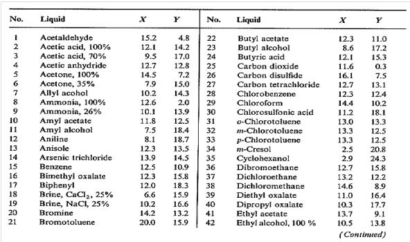
25 What are the factors affecting viscosity: The viscosity of a Newtonian fluid depends mainly on temperature and to a lesser degree on pressure How to calculate the fluid viscosity at different temperatures? 1. For gases: Effect of temperature: The gas viscosity increases with temperature according to the equation: Where: µ = viscosity at absolute temperature T, K = viscosity at 0 ᵒC (273 K) N = complicated parameter and ranges in magnitude from 0.65 to 1 The attached table and graph are used to calculate the gas viscosity at different temperatures and 1 atm pressure. 25

26 How to use this table and figure? Viscosities of gases and vapors at 1 atm 1. Determine the values of x and y according to the gas type from the previous table 2. Plot x and y value on the graph and joint it with the temperature 3. Extend the line to intersect the viscosity scale in a value equals the gas viscosity in cp Effect of pressure: Viscosity of gases is almost independent of pressure in the region of pressure where the gas law applies (i.e. low and moderate pressure). At higher pressures (near the critical point), gas viscosity increases with pressure. 26

27 2. For liquids: Effect of temperature: Liquid viscosity decrease significantly when the temperature is raised. To calculate the liquid viscosity at different temperature by using the attached tables and figures: Effect of pressure: At high pressures (more than 40 atm.) the viscosity of liquid increases with pressure. Units of viscosity: From Newton s law of viscosity: Units of viscosity are: SI system: FPS system: CGS system: = poise, 1 poise = 100 centipoises (cp) Kinematic viscosity: The ratio of the absolute viscosity (µ) to the fluid density is called kinematic viscosity and is designated by (nu). Kinematic viscosities vary with temperature over a narrower range than absolute viscosities. Units of kinematic viscosity =, or Note: 1 = 1 Stoke (1 St.), 1 Stoke = 100 centistokes. Calculation of liquid viscosity at different temperatures By using table and figure similar to that used with gas and with the same procedure. 27

28 28

29 Viscosities of liquids at 1 atm 29

30 Turbulence: What is turbulence? What are the different types of turbulence? Turbulence: is a mass of eddies of various sizes coexisting in the fluid stream, large eddies are continually formed, they break down to smaller eddies and finally disappeared. Types of turbulences: There are two types of turbulences: 1. Wall turbulence: This type occurs due to contact between fluid and solid boundary. Ex: Flow of fluid through closed or open channel or flow of fluid around solid particle (sphere, cylinder, etc.) 2. Free turbulence: This type occurs due to contact between two layers of a fluid flowing at different velocities or contact between two fluids flowing at different velocities (gas sparing or two phase flow) Pressure drop experiment (Reynolds experiment) The purpose of the Reynolds experiment is to: a. Illustrate laminar, transition and fully pipe turbulent flow. b. Determine the conditions under which these types of flow occur. The apparatus is shown in the figure below. Reynolds found that at low flow rates the behaviour of the color band showed clearly that the water was flowing in parallel straight lines and that the flow was laminar. When the flow rate was increased a velocity called the critical velocity was reached at which the thread of colors became wavy and gradually disappeared and that the flow was turbulent. 30

31 Reynolds number and transition from laminar to turbulent flow. Reynold studied the conditions under which one type of flow exists and found that it depends on: 1. Diameter of the tube; D 2. Average velocity of fluid; V 3. Physical properties of the fluid; µ and ρ Furthermore he found that the above factors can be combined in a dimensionless group (form) called Reynolds number (Re) Where: What is Re number? It represents the ratio between inertia force and viscous force. For internal flow (flow in pipes): The flow is laminar when Re <2100 and turbulent when Re>4000 while in the range 2100 < Re < 4000 the flow is transitional. For external flow (flow past flat plate): for Re < 2 х 10 5 the flow is laminar, for Re > 3 х 10 6 the flow is turbulent and for 2 х 10 5 < Re < 3 х 10 6 the flow is transitional. Important note: The general form for writing Reynolds number is Where L is the characteristic length and depends on the solid body which is in contact with the fluid. For flow in pipes or tubes: L is the pipe or tube diameter, For flow past flat plate: L is the plate length in the flow direction, 31

32 For flow around sphere: L is the sphere diameter Note: for other geometries L is the equivalent diameter as it will be seen later. Boundary layer When a fluid flows past a solid surface, the velocity of the fluid in contact with the wall is zero (friction because of viscosity) but rises with increasing distance from the surface and eventually approaches the velocity of the bulk of the stream. If the velocity profile is plotted at different distances from the leading edges (c, c and c ), a sketch similar to the one shown below will be obtained. It is found that almost all the change in velocity occurs in a very thin layer of fluid adjacent to the solid surface: this is known as a boundary layer. As a result, it is possible to treat the flow as two regions: the boundary layer where viscosity has a significant effect, and the region outside the boundary layer, known as the free stream, where viscosity has no direct influence on the flow. Definition of boundary layer: Part of the moving fluid in which the fluid motion is influenced by the presence of a solid boundary Constituents of boundary layer: The boundary layer consists of two parts laminar and turbulent. Near the leading edge of the plate, the flow in the boundary layer is entirely laminar. At distances farther from the leading edge, a point is reached where turbulence appears and after this point turbulent boundary layer exists. 32

33 The turbulent boundary layer consists of three zones namely; viscous sublayer, buffer layer and turbulent core. The fluid velocity near the wall is small and flow in this part of boundary layer is laminar. This part of boundary layer is called viscous sublayer. Farther away from the surface the fluid velocity may be fairly large and flow in this part of boundary layer may become turbulent. This part of boundary layer is called turbulent core. Between the zone of fully developed turbulence and the region of laminar flow is a transition or buffer layer of intermediate character. This part of boundary layer is called buffer layer. Boundary layer thickness Development of turbulent boundary layer on a flat plate Boundary layer thickness is defined as the distance from the wall to the point of 99% of the mean (free) stream velocity. Calculation of boundary layer thickness: 1. For laminar boundary layer 2. For transition boundary layer 3. For turbulent boundary layer where x is the distance from the leading edge and is the boundary layer thickness. Boundary layer formation in straight tube When a fluid enters a tube, a boundary layer begins to form at the wall of the tube. 33

34 As the fluid moves through the tube, the layer thickens and during this stage the boundary layer occupies part of the tube C.S.A. At a point well downstream from the entrance, the boundary layer reaches the center of the tube. At this point the velocity profile in the tube reaches its final form and the flow is called fully developed flow. What is fully developed flow? Flow with constant velocity profile. Important note: Development of boundary layer flow in pipe The length required for the boundary layer to reach the center of the tube and for fully developed flow to be established is called the transition length or entrance length. For laminar flow: For turbulent flow: Boundary layer separation and wake formation Boundary layer separation occurs whenever the change in velocity of the fluid either in magnitude or direction is too large for the fluid to adhere the solid surface. Conditions at which boundary layer separation occurs: 1. Change in the flow channel by Sudden expansion or sudden contraction 2. Sharp bend 3. Obstruction around which the fluid must flow Effect of boundary layer separation on the fluid: In the boundary layer separation zone large eddies called vortices are formed. This zone is known as the wake. The eddies in the wake are kept in motion by the shear stresses between the wake and the separated current. They consume considerable mechanical energy and may lead to a large pressure loss in the fluid. 34

35 How to minimize boundary layer separation? 1. By avoiding sharp changes in the cross sectional area of the flow channel (avoid sudden expansion and sudden contraction) 2. Streamlining any objects over which the fluid must flow. Flow past perpendicular plate Important note: Streamlined shape (minimize wake formation) For enhancing heat transfer or mixing of fluids boundary layer separation may be desirable. 35

36 Basic equations of fluid flow Continuity Equation: What is the continuity equation? What is its importance? What is its mathematical form? The continuity equation is simply a mathematical expression of the principle of conservation of mass that for steady-state flow, the mass flow rate into the system must equal the mass flow rate out. The continuity equation expressed by Equation: For incompressible fluids (ρ is constant) Applications of continuity equation: One of the simplest applications of the continuity equation is determining the change in fluid velocity due to an expansion or contraction in the diameter of a pipe. Important note: Average and local velocity The average velocity ( ) equals the total volumetric flow rate of the fluid divided by the cross section area of the conduit: The local velocity describes the fluid velocity at a certain local position and varies from point to point across the area. The relation between and u Assume differential area ds in the above figure. The mass flow rate is given by the equation: 36

37 but From the above two equations: Examples on continuity equation 1. Steady-state flow exists in a pipe that undergoes a gradual expansion from a diameter of 6 in. to a diameter of 8 in. The density of the fluid in the pipe is constant at 60.8 lbm/ft 3. If the flow velocity is 22.4 ft/sec in the 6 in. section, what is the flow velocity in the 8 in. section? 2. The inlet diameter of the reactor coolant pump is 28 in. while the outlet flow through the pump is 9200 lbm/sec. The density of the water is 49 lbm/ft 3. What is the velocity at the pump inlet? 37

38 3. A piping system has a "Y" configuration for separating the flow as shown in the figure below. The diameter of the inlet leg is 12 in., and the diameters of the outlet legs are 8 and 10 in. The velocity in the 10 in. leg is 10 ft/sec. The flow through the main portion is 500 lbm/sec. The density of water is 62.4 lbm/ft 3. What is the velocity out of the 8 in. pipe section? 38

39 Q: What is the relation between and u and when does u equal? Mass velocity or mass flux Mass flux (G) is the mass flow rate per unit area (mass/area х time) Also (density velocity) Note: Mass velocity or mass flux also called mass current density. Average velocity can be described as the volume flux of the fluid. Mass flux is independent of temperature and pressure for steady state flow. Bernoulli s equation 1. What is Bernoulli equation? 2. How is Bernoulli equation derived? 39

40 3. What are the different forms of Bernoulli equation? 4. What is the importance of or use of Bernoulli equation? What is Bernoulli equation? Bernoulli s equation is a special case of the general energy equation (mechanical energy balance) that is probably the most widely-used tool for solving fluid flow problems. It provides an easy way to relate the elevation head, velocity head, and pressure head of a fluid. How is Bernoulli equation derived? There are two approaches to obtain Bernoulli equation: A. Bernoulli equation is derived based on momentum balance on a control volume. The momentum balance equation states that the sum of all forces acting on the fluid in the direction of flow (one, two or three dimensional flow) equals the rate of momentum change. The momentum balance form is: B. Bernoulli s equation also results from the application of the general energy equation and the first law of thermodynamics to a steady flow system. The general form of the energy balance equation is: (all energies in) = (all energies out) + (energy stored in system) Ein = Eout + E storage Q + (U + PE + KE + PV)in = W + (U + PE + KE + PV)out + (U + PE + KE + PV)stored Bernoulli equation has three different forms: 1. Simplified Bernoulli equation (Bernoulli equation for frictionless flow, ideal flow) Bernoulli s equation results from the application of the general energy equation and the first law of thermodynamics to a steady flow system in which no work is done on or by the fluid, no heat is transferred to or from the fluid, and no change occurs in the internal energy (i.e., no temperature change) of the fluid. Under these conditions, the general energy equation is simplified to: (PE + KE + PV)1 = (PE + KE + PV)2 40

41 Substitution for each term: The above equation is the simplified form of Bernoulli equation and is used for frictionless flow, no work is applied on the fluid and no heat added or lost from the fluid. Each term in Bernoulli equation represents a form of energy possessed by a moving fluid (potential, kinetic, and pressure related energies). In essence, the equation physically represents a balance of the KE, PE, PV energies so that if one form of energy increases, one or more of the others will decrease to compensate and vice versa. Note: Each term of Bernoulli equation has a unit of energy per unit mass (J/kg or lb f ft/lb m ) 41

42 Head form of Bernoulli equation: Multiplying all terms in Bernoulli s equation by the factor results in the form of Bernoulli s equation shown: The units for all the different forms of energy in the above equation are measured in units of distance, these terms are sometimes referred to as "heads" (pressure head, velocity head, and elevation head). Each of the energies possessed by a fluid can be expressed in terms of head. The elevation head represents the potential energy of a fluid due to its elevation above a reference level. The velocity head represents the kinetic energy of the fluid. It is the height in feet that a flowing fluid would rise in a column if all of its kinetic energy were converted to potential energy. The pressure head represents the flow energy of a column of fluid whose weight is equivalent to the pressure of the fluid. The sum of the elevation head, velocity head, and pressure head of a fluid is called the total head. Thus, Bernoulli s equation states that the total head of the fluid is constant. Extended Bernoulli equation 1. Modification for friction (correction of Bernoulli equation for fluid friction): The Bernoulli equation can be modified to take into account the friction losses in the fluid flow to be in the form. Where: F: is the friction loss in the piping system between point 1 and point 2 including both skin and form friction. Question: Compare between skin and form friction V: is the average velocity is the kinetic energy correction factor. It equals ½ for laminar flow and 1 for turbulent flow. Note: 42

43 In the above equation when friction is taken into account u (local velocity) is replaced by V (average velocity). 2. Modification for addition of mechanical work to the fluid (pump work in Bernoulli equation): If the flow line contains a device that adds work to the fluid Bernoulli equation will take the form: Where: is the mechanical work done by the pump per unit mass of fluid and is the pump efficiency. Question: Why is the pump efficiency less than 100%? Because of the presence of friction losses inside the pump between the fluid and the pump body Importance of Bernoulli s equation Bernoulli s equation makes it easy to examine how energy transfers take place among elevation head, velocity head, and pressure head. It is possible to examine individual components of piping systems and determine what fluid properties are varying and how the energy balance is affected. Note: If a pipe containing an ideal fluid undergoes a gradual expansion in diameter, the continuity equation tells us that as the diameter and flow area get bigger, the flow velocity must decrease to maintain the same mass flow rate. Since the outlet velocity is less than the inlet velocity, the velocity head of the flow must decrease from the inlet to the outlet. If the pipe lies horizontal, there is no change in elevation head; therefore, the decrease in velocity head must be compensated for by an increase in pressure head. Since we are considering an ideal fluid that is incompressible, the specific volume of the fluid will not change. The only way that the pressure head for an incompressible fluid can increase is for the pressure to increase. So the Bernoulli equation indicates that a decrease in flow velocity in a horizontal pipe will result in an increase in pressure. Question: If a constant diameter pipe containing an ideal fluid undergoes a decrease in elevation. Explain how energy balance is affected? 43

44 Examples: 1. Assume frictionless flow in a long, horizontal, conical pipe. The diameter is 2.0 ft at one end and 4.0 ft at the other. The pressure head at the smaller end is 16 ft of water. If water flows through this cone at a rate of ft 3 /sec, find the pressure head at the larger end. Solution: By applying Bernoulli s equation between the two ends: Substitute in Bernoulli s equation: 2. Water is pumped from a large reservoir to a point 65 feet higher than the reservoir. How many feet of head must be added by the pump if 8000 lb m /hr flows through a 6-inch pipe and the frictional head loss is 2 feet? The density of the fluid is 62.4 lb m /ft 3 and the pump efficiency is 60%. Assume the kinetic energy correction factor equals 1. Solution: Multiply the above equation by the factor to be in terms of head. 44

45 Where: is the pump head and is the frictional head loss. To use the modified form of Bernoulli s equation, reference points are chosen at the surface of the reservoir (point 1) and at the outlet of the pipe (point 2). The pressure at the surface of the reservoir is the same as the pressure at the exit of the pipe, i.e., atmospheric pressure. The velocity at point 1 will be essentially zero. 45

46 Head loss Head loss is a measure of the reduction in the total head (sum of elevation head, velocity head and pressure head) of the fluid as it moves through a fluid system. Head loss is unavoidable in real fluids. What is the reason of head loss? It is present because of: 1. the friction between the fluid and the walls of the pipe; 2. the friction between adjacent fluid particles as they move relative to one another; and 3. the turbulence caused whenever the flow is redirected or affected in any way by such components as piping entrances and exits, pumps, valves, flow reducers, and fittings. Frictional loss It is that part of the total head loss that occurs as the fluid flows through straight pipes. The head loss for fluid flow is directly proportional to the length of pipe, the square of the fluid velocity, and a term accounting for fluid friction called the friction factor. The head loss is inversely proportional to the diameter of the pipe. Types of friction There are two types of friction losses in the system namely; 1. Skin friction 2. Form friction Skin friction: Objective: To obtain a mathematical relation from which the energy losses due to skin friction can be calculated. Assume a horizontal cylinder through which a non-compressible fluid under the following conditions: 1. Fully developed one dimensional steady state flow 2. Viscous flow (µ = value) 46

47 Fluid element in steady flow through pipe By applying momentum balance equation on a control element in the form of disk of radius (r) and thickness (dl) The forces acting on the element are: Pressure force 1. At a: (+Ve) 2. At b: (-Ve) Shear force = (-Ve) The momentum balance equation is: but (fully developed flow) Important note: The pressure at any given cross section is constant, so that is independent of r. The above equation can be written in the following form: Therefore: 47

48 Relation between skin friction and wall shear stress By applying Bernoulli s equation between points a and b but: Put this value in Bernoulli s equation: Friction factor: (Fanning friction factor) The friction factor is defined as the ratio of the wall shear stress to the product of the velocity head and the density 48

49 The above equation is used to calculate energy losses due to skin friction through the pipeline. This equation is called Darcy s equation To calculate it is necessary to calculate the Fanning friction factor. The friction factor has been determined to depend on the Reynolds number for the flow and the degree of roughness of the pipe s inner surface The quantity used to measure the roughness of the pipe is called the relative roughness, which equals the average height of surface irregularities ( ) divided by the pipe diameter (D). The value of the friction factor is usually obtained from the Moody Chart (shown below). The Moody Chart can be used to determine the friction factor based on the Reynolds number and the relative roughness. Note: are called skin friction parameters. (what is the relation between skin friction parameters) 49

50 For laminar flow: Example: A pipe 100 feet long and 20 inches in diameter contains water at 200 F flowing at a mass flow rate of 700 lb m /sec. The water has a density of 60 lbm/ft3 and a viscosity of x 10-7 lb f - sec/ft 2. The relative roughness of the pipe is Calculate the head loss in ft for the pipe. Form friction: (minor losses) This type of friction occurs in pipelines due to bends, elbows, joints, valves, expansion, contraction etc. The form friction is calculated from the equation: Where k is the losses coefficient: : Expansion coefficient and in general it equals 1 : Contraction coefficient and in general it equals 0.5 : Fitting coefficient. Its value depends on the fitting type as shown in the table below Losses coefficient for standard threaded fittings 50

51 Important note: We can write a general equation for the total friction losses in the form: and the total friction head: Shear stress and velocity distribution in pipelines under laminar flow conditions: Required: Derive an expression for shear stress distribution in a pipeline and sketch it (for Newtonian fluid). From the two equations: The above relation represents the shear stress distribution equation (for laminar and turbulent flow). It represents a straight line equation of slope Sketch of shear stress distribution: Variation of shear stress in pipe 51

52 Question: Prove that the shear stress distribution in a pipeline follows a straight line equation. Velocity distribution in laminar flow in pipeline: Required: velocity distribution, relation between maximum velocity and average velocity Assume a ring of Newtonian fluid of radius r and thickness dr. For Newtonian fluids: But from the shear stress distribution equation: From the above two equations: The above equation is the velocity distribution equation for Newtonian fluid under laminar flow conditions in pipeline. The velocity distribution takes the form shown by the figure below. 52

53 Maximum velocity The maximum velocity occurs at r = 0.0 Relation between local and maximum velocity Average velocity The relation between the average and local velocity is: The relation between average and maximum velocity Hagen-Poiseuille equation: In fluid dynamics, the Hagen Poiseuille equation is a physical law that gives the pressure drop in a fluid flowing through a long cylindrical pipe. The assumptions of the equation are that the fluid is viscous and incompressible; the flow is laminar through a pipe of constant circular crosssection that is substantially longer than its diameter; and there is no acceleration of fluid in the pipe. The equation is also known as the Hagen Poiseuille law, Poiseuille law and Poiseuille equation. Derivation of the equation: 53

54 The above equation is the Hagen-Poiseuille equation and is used to calculate the fluid viscosity by knowing the other parameters. The assumptions of the equation are that: The fluid is viscous and incompressible; The flow is laminar and fully developed through a pipe of constant circular cross-section that is substantially longer than its diameter; Smooth pipe Note regarding Reynolds number For flow through no circular cross sectional area: where is the equivalent diameter and is calculated from the equation: Questions: 1. Derive an expression for the viscous shear stress distribution for Newtonian fluid flowing through a horizontal pipe. Sketch the shear stress distribution. 2. Derive an equation for the local velocity distribution for Newtonian fluid flowing through a horizontal pipe. Obtain an expression for the maximum velocity. 3. Prove that for laminar flow in pipes. 4. What is Hagen-Poiseuille equation? When is it used? 54

55 Some notes about pump calculations and pipes dimensions Some Important Terminologies 1. Static Suction Lift (SSL) The distance measured vertically the intake of the pump or the pump is placed above the surface of the liquid in the suction tank. 2. Static Suction Head (SSH) The distance measured vertically the pump is placed below the surface of the liquid in the suction tank. 3. Static Discharge Head (SDH) The distance measured vertically the pump is placed below the surface of the liquid in the discharge tank. 4. Total Static Head The vertical distance from the surface of the liquid in the suction tank to the surface of the liquid in the discharge tank. TSH = SSL + SDH TSH = SDH - SSH 55

56 Pump developed head: Bernoulli equation can be written between point (a) and (b) The term is the total suction head and the term 22 is the total discharge head. The difference between the total discharge head and the total suction head is the developed head H. Power requirements 1. Power supplied to the pump: 2. Power delivered to the fluid: Pipeline specifications: Pipes are specified by two parameters, namely; inside diameter and wall thickness. Pipes are now specified according to wall thickness by a standard formula for schedule number as designated by the American Standards Association. Schedule number is defined by the American Standards Association as the approximate value of See appendix for dimensions of standard steel pipes 56

57 Net Positive Suction Head NPSH Definition: Net positive suction head is the term that is usually used to describe the absolute pressure of a fluid at the inlet to a pump minus the vapor pressure of the liquid. The resultant value is known as the Net Positive Suction Head available. The term is normally shortened to the acronym NPSH A, the A denotes available. A similar term is used by pump manufactures to describe the energy losses that occur within many pumps as the fluid volume is allowed to expand within the pump body. This energy loss is expressed as a head of fluid and is described as NPSH R (Net Positive Suction Head requirement) the R suffix is used to denote the value is a requirement. Different pumps will have different NPSH requirements dependant on the impellor design, impellor diameter, inlet type, flow rate, pump speed and other factors. Pressure at the pump inlet The fluid pressure at a pump inlet will be determined by the pressure on the fluid surface, the frictional losses in the suction pipework and any rises or falls within the suction pipework system. NPSH A calculation The elements used to calculate NPSHa are all expressed in absolute head units. The NPSHa is calculated from: For suction head Fluid surface pressure + positive head pipework friction loss fluid vapour pressure 57

58 For suction lift Fluid surface pressure - negative head pipework friction loss fluid vapour pressure Important note: For safe pump operation and to avoid cavitation: What is cavitation? The process of the formation and subsequent collapse of vapor bubbles in a pump is called cavitation. Effect of cavitation on pump performance Three effects of pump cavitation are: Degraded pump performance resulting in a fluctuating flow rate and discharge pressure Excessive pump vibration Destructive to pump internal components (damage to pump impeller, bearings, wearing rings, and seals) Example: Benzene at 38.7 ᵒC is pumped through the system shown in the figure below at the rate of 9.09 m 3 /h. The reservoir is at atmospheric pressure. The gauge pressure at the end of the discharge line is 345 kn/m 2. The discharge is 10 ft and the pump suction 4 ft above the level in the reservoir. The discharge line is Schedule 40 pipe. The friction in the suction line is known to be 3.45 kn/m 2 and that in the discharge line is 37.9 kn/m 2. The mechanical efficiency of the pump is 60%. The density of benzene is 865 kg/m 3 and its vapor pressure at 38.7 ᵒC is 26.2 kn/m 2. Calculate: 1. The developed head of the pump 2. The total power input 3. The NPSH A 58

59 Dimensional Analysis What is dimensional analysis? Application of the law of conservation of dimensions to arrange the variables that are important in a given problem into a set of dimensionless groups used to define the system behavior. Dimensional analysis involves grouping the variables in a given situation into dimensionless parameters that are less numerous than the original variables. It is important to realize that the process of dimensional analysis only replaces the set of original (dimensional) variables with an equivalent (smaller) set of dimensionless variables (i.e., the dimensionless groups). It does not tell how these variables are related the relationship must be determined either theoretically by application of basic scientific principles or empirically by measurements and data analysis. However, dimensional analysis is a very powerful tool in that it can provide a direct guide for experimental design and scale-up and for expressing operating relationships in the most general and useful form. Advantages of dimensional analysis: 1. Dimensionless quantities are universal so any relationship involving dimensionless variable is independent of the size or scale of the system. It will be a useful tool for scale up (translate data from laboratory models (proto type) to large scale equipment. 2. The relations that define the behavior of a given system are much simpler when expressed in terms of the dimensionless variables. In other words, the amount of effort required to represent a relationship between the dimensionless groups is much less than that required relating each of the variables independently, and the resulting relation will thus be simpler in form. Dimensions: In dimensional analysis certain dimensions must be established as fundamentals. One of these fundamental dimensions is: 59

60 Variable Symbolized Length L Mass M Time t The significant quantities in momentum transfer can be all expressed dimensionally in terms of L, M and t. For example: Quantity Dimensional expression Velocity L/t Acceleration L/t 2 Area L 2 Force ML/t 2 Pressure M/Lt 2 Viscosity M/Lt Dimensional analysis steps: There are a number of different approaches to dimensional analysis. The classical method is the Buckingham Theorem, so-called because Buckingham used the symbol to represent the dimensionless groups. Another classic approach, which involves a more direct application of the law of conservation of dimensions, is attributed to Lord Rayleigh. The following is a brief outline to the main steps involved in dimensional analysis. 1. Identify the important variables in the system (this can be determined through common sense, intuition or experience. They can also be determined from a knowledge of the physical principles that govern the system (e.g., the conservation of mass, energy, momentum, etc., as written for the specific system to be analyzed) along with the fundamental equations that describe these principles) 2. List all the problem variables and parameters, along with their dimensions (The number of dimensionless groups that will be obtained is equal to the number of variables less the minimum number of fundamental dimensions involved in these variables) 3. Choose a set of reference variables 60

61 4. Solve the dimensional equations for the dimensions (L, M and t) in terms of the reference variables 5. Write the dimensional equations for each of the remaining variables in terms of the reference variables 6. The resulting equations are each a dimensional identity, so dividing one side by the other results in one dimensionless group from each equation Examples: Ex (1): Pipeline analysis The procedure for performing a dimensional analysis will be illustrated by means of an example concerning the flow of a liquid through a circular pipe. In this example we will determine an appropriate set of dimensionless groups that can be used to represent the relationship between the flow rate of an incompressible fluid in a pipeline, the properties of the fluid, the dimensions of the pipeline, and the driving force for moving the fluid, as illustrated in Fig. 1. The procedure is as follows. Fig. 1, Flow in pipeline 1. Identify the important variables in the system The important variables are: (where is the surface roughness) 2. List all the problem variables and parameters, along with their dimensions Quantity Dimensional expression V L/t M/Lt 2 D L L L L M/L 3 M/Lt 61