Lecture2 The implicit function theorem. Bifurcations.

Transcription

1 Lecture2 The implicit function theorem. Bifurcations.

2 1 Review:Newton s method. The existence theorem - the assumptions. Basins of attraction. 2 The implicit function theorem. 3 Bifurcations of iterations. Attractors and repellers The fold. The period doubling bifurcation. 4 Graphical iteration.

3 Newton s method. This is an algorithm to find the zeros of a function P = P(x). Starting with an initial point x 0 inductively define (or rather try to define) x n+1 = x n P(x n) P (x n ). (1)

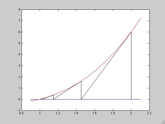
4 Recall the graphic illustration of Newton s method: Notice that what we are doing is taking the tangent to the curve at the point (x, y) and then taking as our next point, the intersection of this tangent with the x-axis. This makes the method easy to remember.

5 T

6 A fixed point of the iteration scheme is a solution to our problem. Also notice that if x is a fixed point of this iteration scheme, i.e. if x = x P(x) P (x) then P(x) = 0 and we have a solution to our problem. To the extent that x n+1 is close to x n we will be close to a solution (the degree of closeness depending on the size of P(x n )).

7 The existence theorem - the assumptions. For the purposes of formulation and proof, in order to simplify the notation, let us assume that we have shifted our coordinates so as to take x 0 = 0. Also let B = {x : x 1}. We need to assume that P (x) is nowhere zero, and that P (x) is bounded. In fact, we assume that there is a constant K such that P (x) 1 K, P (x) K, x B. (2)

8 The existence theorem - the assumptions. We proved: Proposition. Let τ = 3 2 and choose the K in (2) so that K 23/4. Let c = 8 ln K. 3 Then if P(0) K 5 (3) the recursion (1) starting with x 0 = 0 satisfies x n B n (4) and x n x n 1 e cτ n. (5)

9 The existence theorem - the assumptions. A more general theorem. To prove: and x n B n (4) x n x n 1 e cτ n. (5) In fact, we will prove a somewhat more general result. So we will let τ be any real number satisfying 1 < τ < 2 and we will choose c in terms of K and τ to make the proof work. First of all we notice that (4) is a consequence of (5) if c is sufficiently large. In fact, so x j = (x j x j 1 ) + + (x 1 x 0 )

10 The existence theorem - the assumptions. x j x j x j x 1 x 0. Using (5) for each term on the right gives x j j e cτ n < 1 e cτ n < 1 e cn(τ 1) = 1 e c(τ 1) 1 e c(τ 1). Here the third inequality follows from writing by the binomial formula τ = 1 + (τ 1) so τ n = 1 + n(τ 1) + > n(τ 1) since τ > 1. The equality is obtained by summing the geometric series.

11 The existence theorem - the assumptions. x j e c(τ 1) 1 e c(τ 1). So if we choose c sufficiently large that e c(τ 1) 1 (6) 1 e c(τ 1) (4) follows from (5). This choice of c is conditioned by our choice of τ. But at least we now know that if we can arrange that (5) holds, then by choosing a possibly larger value of c (and if we can still prove that (5) continues to hold) we can guarantee that the algorithm keeps going.

12 The existence theorem - the assumptions. So let us try to prove (5) by induction. If we assume it is true for n, we may write x n+1 x n = S n P(x n ) where we set S n = P (x n ) 1. (7) We use the first inequality in (2) which says that P (x) 1 K, and the definition (1) for the case n 1 (which says that x n = x n 1 S n 1 P(x n 1 )) to get S n P(x n ) K P(x n 1 S n 1 P(x n 1 )). (8)

13 The existence theorem - the assumptions. S n P(x n ) K P(x n 1 S n 1 P(x n 1 )). (8) Taylor s formula with remainder says that for any twice continuously differentiable function f, f (y+h) = f (y)+f (y)h+r(y, h) where R(y, h) 1 2 sup f (z) h 2 z where the supremum is taken over the interval between y and y + h. If we use Taylor s formula with remainder with f = P, y = P(x n 1 ), and h = S n 1 P(x n 1 ) = x n x n 1 and the second inequality in (2) to estimate the second derivative, we obtain P(x n 1 S n 1 P(x n 1 )) P(x n 1 ) P (x n 1 )S n 1 P(x n 1 ) + K x n x n 1 2.

14 The existence theorem - the assumptions. P(x n 1 S n 1 P(x n 1 )) P(x n 1 ) P (x n 1 )S n 1 P(x n 1 ) + K x n x n 1 2. Substituting this inequality into (8), we get x n+1 x n K P(x n 1 ) P (x n 1 )S n 1 P(x n 1 ) + K 2 x n x n 1 2. (9) Now since S n 1 = P (x n 1 ) 1 the first term on the right vanishes and we get x n+1 x n K 2 x n x n 1 2 K 2 e 2cτ n.

15 The existence theorem - the assumptions. Choosing c so that the induction works. x n+1 x n K 2 x n x n 1 2 K 2 e 2cτ n. So in order to pass from n to n + 1 in (5) we must have K 2 e 2cτ n cτ n+1 e or K 2 e c(2 τ)τ. (10) Since τ < 2 we can arrange for this last inequality to hold if we choose c sufficiently large.

16 The existence theorem - the assumptions. Getting started. To get started, we must verify (5) for n = 1 This says S 0 P(0) e cτ or So we have proved: P(0) e cτ K. (11)

17 The existence theorem - the assumptions. Theorem P (x) 1 K, P (x) K, x B. (2) e c(τ 1) 1 (6) 1 e c(τ 1) K 2 e c(2 τ)τ. (10) P(0) e cτ K. (11) Suppose that (2) holds and we have chosen K and c so that (6) and (10) hold. Then if P(0) satisfies (11) the Newton iteration scheme converges exponentially in the sense that (5) holds. x n x n 1 e cτ n. (5)

18 The existence theorem - the assumptions. If we choose τ = 3 2 as in the proposition, let c be given by K 2 = e 3c/4 so that (10) just holds. This is our choice in the proposition. The inequality K 2 3/4 implies that e 3c/4 4 3/4 or This implies that so (6) holds. Then e c 4. e c/2 1 2 e cτ = e 3c/2 = K 4 so (11) becomes P(0) K 5 completing the proof of the proposition.

19 The existence theorem - the assumptions. Review. We have put in all the gory details, but it is worth reviewing the guts of the argument, and seeing how things differ from the special case of finding the square root. Our algorithm is x n+1 = x n S n [P(x n )] (12) where S n is chosen as (7). Taylor s formula gave (9) and with the choice (7) we get x n+1 x n K 2 x n x n 1 2. (13)

20 The existence theorem - the assumptions. In contrast to the square root algorithm, we can t conclude that the error vanishes as r τ n with τ = 2. But we can arrange that we eventually have such exponential convergence with any τ < 2.

21 Basins of attraction. The more decisive difference has to do with the basins of attraction of the solutions. For the square root, starting with any positive number ends us up with the positive square root. Every negative number leads us to the negative square root. So the basin of attraction of the positive square root is the entire positive half axis, and the basin of attraction of the negative square root is the entire negative half axis. The only bad point belonging to no basin of attraction is the point 0. Even for cubic polynomials the global behavior of Newton s method is extraordinarily complicated, as we saw last time.

22 Verifying the conditions. Let us return to the positive aspect of Newton s method. You might ask, how can we ever guarantee in advance that an inequality such as (3) holds? The answer comes from considering not a single function, P, but rather a parameterized family of functions: Suppose that u ranges over some interval, or more generally, over some region in a vector space. To fix the notation, suppose that this region contains the origin, 0. Suppose that P is a function of u and x, and depends continuously on (u, x). Suppose that as a function of x, the function P is twice differentiable and satisfies (2) for all values of u (with the same fixed K). ( ) P 1 x K, 2 P (x) 2 K, x B, u. (2)

23 Finally, suppose that P(0, 0) = 0. (14) Then the continuity of P guarantees that for u and x 0 sufficiently small, the condition (3) holds, that is P(u, x 0 ) < r where r is small enough to guarantee that x 0 is in the basin of attraction of a zero of the function P(u, )

24 In particular, this means that for u sufficiently small, we can find an ɛ > 0 such that all x 0 satisfying x 0 < ɛ are in the basin of attraction of the same zero of P(u, ). By choosing a smaller neighborhood, given say by u < δ, starting with x 0 = 0 and applying Newton s method to P(u, ), we obtain a sequence of x values which converges exponentially to a solution of P(u, x) = 0. (15) satisfying x < ɛ.

25 The implicit function theorem. Furthermore, starting with any x 0 satisfying x 0 < ɛ we also get exponential convergence to the same zero. In particular, there can not be two distinct solutions to (15) satisfying x < ɛ, since starting Newton s method at a zero gives (inductively) x n = x 0 for all n. Thus we have constructed a unique function x = g(u) satisfying P(u, g(u)) 0. (16) This is the guts of the implicit function theorem.

26 This is the guts of the implicit function theorem. We have proved it under assumptions which involve the second derivative of P which are not necessary for the truth of the theorem. (We will remedy this later in the course.) However these stronger assumptions that we have made do guarantee exponential convergence of our algorithm. For the sake of completeness, we discuss the basic properties of the function g: its continuity, differentiability, and the computation of its derivative.

27 Continuity of the implicit function, g. We wish to prove that g is continuous at any point u in a neighborhood of 0. This means: given β > 0 we can find α > 0 such that h < α g(u + h) g(u) < β. (17) We know that this is true at u = 0, where we could choose any ɛ > 0 at will, and then conclude that there is a δ > 0 with g(u) < ɛ if u < δ.

28 Uniqueness implies continuity at a general point. To prove: given β > 0 we can find α > 0 such that h < α g(u + h) g(u) < β. (17) To prove (17) at a general point, just choose (u, g(u)) instead of (0, 0) as the origin of our coordinates, and apply the preceding results to this new data. We obtain a solution f to the equation P(u + h, f (u + h)) = 0 with f (u) = g(u) which is continuous at h = 0. In particular, for h sufficiently small, we will have u + h δ, and f (u + h) < ɛ, our original ɛ and δ in the definition of g. The uniqueness of the solution to our original equation then implies that f (u + h) = g(u + h), proving (17).

29 Differentiability of g. Suppose that P is continuously differentiable with respect to all variables. We have 0 P(u + h, g(u + h)) P(u, g(u) so, by the definition of the derivative, 0 = P u h + P [g(u + h) g(u)] + o(h) + o[g(u + h) g(u)]. x If u is a vector variable, say R n, then P u is a matrix. The terminology o(s) means some expression which approaches zero so that o(s)/s 0. So [ ] P 1 [ ] [ ] P P 1 g(u+h) g(u) = h o(h) o[g(u+h) g(u)]. x u x (18)

30 g(u+h) g(u) = [ P x ] 1 [ ] P h o(h) u [ ] P 1 o[g(u+h) g(u)]. x As a first pass through this equation, observe that by the continuity that we have already proved, we know that [g(u + h) g(u)] 0 as h 0. The expression o([g(u + h) g(u)]) is, by definition of o, smaller than any constant times g(u + h) g(u) provided that g(u + h) g(u) itself is sufficiently small. This means that for sufficiently small [g(u + h) g(u)] we have o[g(u + h) g(u)] 1 g(u + h) g(u) 2K where we may choose K so that [ ] P 1 x K.

31 g(u+h) g(u) = [ P x ] 1 [ ] P h o(h) u [ ] P 1 o[g(u+h) g(u)]. x o[g(u + h) g(u)] 1 g(u + h) g(u) 2K where we may choose K so that [ ] P 1 x K. So bringing the last term over to the other side gives g(u+h) g(u) 1 [ ] P 1 [ ] P 2 g(u+h) g(u) h +o( h ), x u and we get an estimate of the form for some suitable constant, M. g(u + h) g(u) M h

32 g(u+h) g(u) = [ P x ] 1 [ ] P h o(h) u g(u + h) g(u) M h. [ ] P 1 o[g(u+h) g(u)]. x So the term o[g(u + h) g(u)] becomes o(h). Plugging this back into our equation (18) shows that g is differentiable with g u = [ P x ] 1 [ ] P. (19) u

33 To summarize, the implicit function theorem says: Theorem The implicit function theorem. Let P = P(u, x) be a differentiable function with P(0, 0) = 0 and [ ] P x (0, 0) invertible. Then there exist δ > 0 and ɛ > 0 such that P(u, x) = 0 has a unique solution with x < ɛ for each u < δ. This defines the function x = g(u). The function g is differentiable and its derivative is given by (19). g u = [ P x ] 1 [ ] P. (19) u

34 [ ] g P 1 [ ] P u =. (19) x u We have proved the theorem under more stringent hypotheses in order to get an exponential rate of convergence to the solution. We will provide the details of the more general version, as a consequence of the contraction fixed point theorem, later on. We should point out now, however, that nothing in our discussion of Newton s method or the implicit function theorem depended on x being a single real variable. The entire discussion goes through unchanged if x is a vector variable. Then P/ x is a matrix, and (19) must be understood as matrix multiplication. Similarly, the condition on the second derivative of p must be understood in terms of matrix norms. We will return to these points later. For now I want to give some interesting applications of the implicit function theorem.

35 Over the next few lectures I want to study the behavior of iterations of a map of an interval of the real line into the real line. But we will let this map depend on a parameter. So we will be studying the iteration (in x) of a function, F, of two real variables x and µ. We will need to make various hypothesis concerning the differentiability of F. We will always assume it is at least C 2 (has continuous partial derivatives up to the second order). We may also need C 3 in which case we explicitly state this hypothesis. We write F µ (x) = F (x, µ) and are interested in the change of behavior of F µ as µ varies.

36 The logistic family. A very famous example is the logistic family of maps, where F (x, µ) = µx(1 x). For any fixed value of µ, the maximum of F (x, µ) as a function of x is achieved at x = 1 2 and the maximum value is 1 4 µ. On the other hand, F (x, µ) 0 when µ 0 and 0 x 1. So for any value of µ with 0 µ 4, the map x F µ (x) maps the unit interval into itself. But, as many of you have undoubtedly seen, the behavior of this map changes drastically as µ varies. I plan to study this example in detail in the next lecture.

37 Attractors and repellers A single map. Let me begin by studying the case of a single map. In other words we are holding µ fixed. Here is some notation which we will be using for the next few lectures: Let f : X X be a differentiable map where X is an interval on the real line. A point p X is called a fixed point if f (p) = p.

38 Attractors and repellers Attractive fixed points. A fixed point a is called an attractor or an attractive fixed point or a stable fixed point if f (a) < 1. (20) The reason for this terminology is that points sufficiently close to an attractive fixed point, a, converge to a geometrically upon iteration.

39 Attractors and repellers An attractive fixed point attracts nearby points. Points sufficiently close to an attractive fixed point, a, converge to a geometrically upon iteration. Indeed, f (x) a = f (x) f (a) = f (a)(x a) + o(x a) by the definition of the derivative. Hence taking b < 1 to be any number larger than f (a) then for x a sufficiently small, f (x) a b x a. So starting with x 0 = x and iterating x n+1 = f (x n ) gives a sequence of points with x n a b n x a.

40 Attractors and repellers The basin of attraction. The basin of attraction of an attractive fixed point is the set of all x such that the sequence {x n } converges to a where x 0 = x and x n+1 = f (x n ). Thus the basin of attraction of an attractive fixed point a will always include a neighborhood of a, but it may also include points far away, and may be a very complicated set as we saw in the example of Newton s method applied to a cubic.

41 Attractors and repellers Repellers. A fixed point, r, is called a repeller or a repelling or an unstable fixed point if f (r) > 1. (21) Points near a repelling fixed point are pushed away upon iteration.

42 Attractors and repellers Superattractors. An attractive fixed point s with f (s) = 0 (22) is called superattractive or superstable. Near a superstable fixed point, s, the iterates converge faster than any geometrical rate to s.

43 Attractors and repellers For example, in Newton s method, so f (x) = x P(x) P (x) f (x) = 1 P (x) P (x) + P(x)P (x) (P (x) 2 = P(x)P (x) P (x) 2. So if a is a zero of P, then it is a superattractive fixed point.

44 Attractors and repellers Notation for iteration. The notation f n will mean the n-fold composition, f n = f f f (ntimes).

45 Attractors and repellers Periodic points. A fixed point of f n is called a periodic point of period n. If p is a periodic point of period n, then so are each of the points p, f (p), f 2 (p),..., f (n 1) (p) and the chain rule says that at each of these points the derivative of f n is the same and is given by (f n ) (p) = f (p)f (f (p)) f (f (n 1) (p)). If any one of these points is an attractive fixed point for f n then so are all the others. We speak of an attractive periodic orbit. Similarly for repelling.

46 Attractors and repellers A periodic point will be superattractive for f n if and only if at least one of the points p, f (p),... f (n 1) (p) satisfies f ( q) = 0.

47 Attractors and repellers Repeat of hypotheses. We will be studying the iteration (in x) of a function, F, of two real variables x and µ. We will need to make various hypothesis concerning the differentiability of F. We will always assume it is at least C 2 (has continuous partial derivatives up to the second order). We may also need C 3 in which case we explicitly state this hypothesis. We write F µ (x) = F (x, µ) and are interested in the change of behavior of F µ as µ varies.

48 Attractors and repellers Stability of attractors or repellors. Before embarking on the study of bifurcations let us observe that if p is a fixed point of F µ and F µ(p) 1, then for ν close to µ, the transformation F ν has a unique fixed point close to p. Indeed, the implicit function theorem applies to the function P(x, ν) := F (x, ν) x since P (p, µ) 0 x by hypothesis. We conclude that there is a curve of fixed points x(ν) with x(µ) = p.

49 The fold. The fold bifurcation. The first type of bifurcation we study is the fold bifurcation where there is no (local) fixed point on one side of the bifurcation value, b, where a fixed point p appears at µ = b with F µ(p) = 1, and at the other side of b the map F µ has two fixed points, one attracting and the other repelling.

50 The fold. Example: the quadratic family. As an example consider the quadratic family Q(x, µ) = Q µ (x) := x 2 + µ. Fixed points must be solutions of the quadratic equation x 2 x + µ = 0, whose roots are p ± = 1 2 ± µ. So for µ > 1 4 there are no real fixed points. At µ = 1 4 there is a single fixed point at x = 1 2. Since f (x) = 2x, we have f ( 1 2) = 1. For µ slightly less than 1 4 there are two fixed points, one at slightly more than 1 2 where the derivative is > 1 and so is repelling, and one at slightly less than 1 2 which is an attractor.

51 The fold. The quadratic family at µ =.5,.25, and 0. Remember that a fixed point of f is a point where the graph of f intersects the line y = x.

52 The fold. We will now discuss the general phenomenon. In order not to clutter up the notation, we assume that coordinates have been chosen so that b = 0 and p = 0. So we make the standing assumption that p = 0 is a fixed point at µ = 0, i.e. that F (0, 0) = 0.

53 The fold. Theorem (Fold bifurcation). Suppose that at the point (0, 0) we have (a) F x (0, 0) = 1, (b) 2 F F (0, 0) > 0, (c) (0, 0) > 0. x 2 µ Then there are non-empty intervals (µ 1, 0) and (0, µ 2 ) and ɛ > 0 so that (i) If µ (µ 1, 0) then F µ has two fixed points in ( ɛ, ɛ). One is attracting and the other repelling. (ii) If µ (0, µ 2 ) then F µ has no fixed points in ( ɛ, ɛ).

54 The fold. Proof of the fold bifurcation theorem, I. All the proofs in this section will be applications of the implicit function theorem. For our current theorem, set P(x, µ) := F (x, µ) x. Then by our standing hypothesis we have and condition (c) says that P(0, 0) = 0 P (0, 0) > 0. µ The implicit function theorem gives a unique function µ(x) with µ(0) = 0 and P(x, µ(x)) 0.

55 The fold. Proof of the fold bifurcation theorem, II. The implicit function theorem gives a unique function µ(x) with µ(0) = 0 and P(x, µ(x)) 0. The formula for the derivative in the implicit function theorem gives µ (x) = P/ x P/ µ which vanishes at the origin by assumption (a). We then may compute the second derivative, µ, via the chain rule; using the fact that µ (0) = 0 we obtain µ (0) = 2 P/ x 2 (0, 0). P/ µ This is negative by assumptions (b) and (c).

56 The fold. Proof of the fold bifurcation theorem, III. In other words, µ (0) = 0, and µ (0) < 0 so µ(x) has a maximum at x = 0, and this maximum value is 0. In the (x, µ) plane, the graph of µ(x) looks locally approximately like a parabola in the lower half plane with its apex at the origin. If we rotate this picture clockwise by ninety degrees, this says that there are no points on this curve sitting over positive µ values, i.e. no fixed points for positive µ, and two fixed points for µ < 0.

57 The fold. Graph of the function x µ(x).

58 The fold. Rotated figure.

59 The fold. Proof of the fold bifurcation theorem, IV We have established that for µ small there are two fixed points for µ < 0 and no fixed points for µ > 0. We must now show that one of these fixed points is attracting and the other repelling. For this, consider the function F x (x, µ(x)). The derivative of this function with respect to x is 2 F x 2 (x, µ(x)) + 2 F x µ (x, µ(x))µ (x). Assumption (b) says that 2 F x 2 (0, 0) > 0, and we know that µ (0) = 0. So the above expression is positive at 0.

60 The fold. Completion of the proof of the fold bifurcation theorem. We know that F x (x, µ(x)) is an increasing function in a neighborhood of the origin while F x (0, 0) = 1. But this says that on the lower fixed point and F µ(x) < 1 F µ(x) > 1 at the upper fixed point, completing the proof of the theorem.

61 The fold. In conditions (b) and (c) of the theorem, we could have allowed (separately) negative instead of positive values. This allows for the possibility that the two fixed points appear to the right (instead of the left) of the origin and that the upper (rather that the lower) fixed point is the attractor.

62 The period doubling bifurcation. Description of the period doubling bifurcation. The fold bifurcation arises when the parameter µ passes through a value where F µ (x) = x and F µ(x) = 1. Under the appropriate hypotheses, the period doubling bifurcation describes what happens when µ passes through a bifurcation value b where F b (x) = x and F µ(x) = 1. On one side of b there is a single attractive fixed point. On the other side the attractive fixed point has become a repelling fixed point, and an attractive periodic point of period two has arisen. This is illustrated in the figure in the next frame.

63 The period doubling bifurcation " attracting double point repelling fixed point!! attracting fixed point µ

64 The period doubling bifurcation. I will give the statement and proof of the period doubling bifurcation after we have given one of the most famous examples of this phenomenon - the case of the logistic family.

65 Iteration for kindergarten. Suppose that we have drawn a graph of the map f, and have also drawn the x-axis and the diagonal line y = x. The iteration of f starting with an initial point x 0 on the x-axis can be visualized as follows: Draw the vertical line from x 0 until it hits the graph (at (x 0, f (x 0 )). Draw the horizontal line to the diagonal (at f (x 0 ), f (x 0 )). Call this new x value x 1, so x 1 = f (x 0 ). Draw the vertical line to the graph (at (x 1, f (x 1 )). Continue. We illustrate this for the graphical iteration of the quadratic map f (x) = x starting with the initial point.75. Notice that we are moving away from the unstable fixed point.

66 The first few steps of the graphical iteration, leading away from the repelling fixed point.

67 More iterations lead to the attractive fixed point.