PID Tuning of Plants With Time Delay Using Root Locus

Transcription

1 San Jose State University SJSU ScholarWorks Master's Theses Master's Theses and Graduate Research Summer 2011 PID Tuning of Plants With Time Delay Using Root Locus Greg Baker San Jose State University Follow this and additional works at: Recommended Citation Baker, Greg, "PID Tuning of Plants With Time Delay Using Root Locus" (2011). Master's Theses This Thesis is brought to you for free and open access by the Master's Theses and Graduate Research at SJSU ScholarWorks. It has been accepted for inclusion in Master's Theses by an authorized administrator of SJSU ScholarWorks. For more information, please contact

2 PID-TUNING OF PLANTS WITH TIME DELAY USING ROOT LOCUS A Thesis Presented to The Faculty of the Department of General Engineering San José State University In Partial Fulfillment of the Requirements for the Degree Master of Science by Greg Baker August 2011

3 2011 Greg Baker ALL RIGHTS RESERVED

4 The Designated Thesis Committee Approves the Thesis Titled PID-TUNING OF PLANTS WITH TIME DELAY USING ROOT LOCUS by Greg Baker APPROVED FOR THE DEPARTMENT OF GENERAL ENGINEERING SAN JOSÉ STATE UNIVERSITY August 2011 Dr. Peter Reischl Department of Electrical Engineering Dr. Ping Hsu Department of Electrical Engineering Dr. Julio Garcia Department of Aviation and Technology

5 ABSTRACT PID-TUNING OF PLANTS WITH TIME DELAY USING ROOT LOCUS by Greg Baker This thesis research uses closed-loop pole analysis to study the dynamic behavior of proportional-integral-derivative (PID) controlled feedback systems with time delay. A conventional tool for drawing root loci, the MATLAB function rlocus() cannot draw root loci for systems with time delay, and so another numerical method was devised to examine the appearance and behavior of root loci in systems with time delay. Approximating the transfer function of time delay can lead to a mismatch between a predicted and actual response. Such a mismatch is avoided with the numerical method developed here. The method looks at the angle and magnitude conditions of the closedloop characteristic equation to identify the true positions of closed-loop poles, their associated compensation gains, and the gain that makes a time-delayed system become marginally stable. Predictions for system response made with the numerical method are verified with a mathematical analysis and cross-checked against known results. This research generates tuning coefficients for proportional-integral (PI) control of a first-order plant with time delay and PID control of a second-order plant with time delay. The research has applications to industrial processes, such as temperature-control loops.

6 ACKNOWLEDGEMENTS This thesis was produced with the help of several individuals. First, the author is indebted to the inspirational instruction of Dr. Peter Reischl, and the willingness of Mr. Owen Hensinger to share his experience in process control, the source of the overshootreduction technique suggested in the text. Sincere appreciation is expressed for the guidance and counsel of Dr. Ping Hsu and Dr. Julio Garcia. Lifelong thanks are due for the patience and support of my wife Adrienne Harrell.

7 TABLE OF CONTENTS 1.0 Introduction 1 The Problems With Time Delay 3 PID Compensation 10 Review of PID-Tuning Approaches for Systems With Time Delay 13 PID-Tuning Approach for Systems With Time Delay Used in This Study Validation of Numerical Algorithm 17 Proportional Compensation of First- and Second-Order Plants Without Time Delay Results 26 Proportional Compensation of a First-Order Plant With Time Delay 26 Proportional-Integral (PI) Compensation of a First-Order Plant Without Time Delay Proportional-Integral (PI) Tuning Strategy With and Without Time Delay Proportional-Integral (PI) Compensation of a First-Order Plant With Time Delay Proportional-Integral (PI) Coefficients for a First-Order Plant With Time Delay Proportional-Integral-Derivative (PID) Compensation of a Second- Order Plant Without Time Delay Proportional-Integral-Derivative (PID) Compensation of a Second- Order Plant With Time Delay Proportional-Integral-Derivative (PID) Coefficients for a Second- Order Plant With Time Delay vi

8 4.0 Conclusion 56 References 59 Appendices 62 Appendix A: Laplace Transform 62 Appendix B: Inverse Laplace Transform and Residue Theorem 63 Appendix C: Tools 65 Appendix D: Identifying the Poles and Zeros of a PID Compensator 70 Appendix E: Numerical Computation of Root Locus With and Without Time Delay Appendix F: Root Loci for Simple Plants Drawn Using Approximated Time Delay Appendix G: Root Loci for Simple Plants Drawn Using True Time Delay Appendix H: Compensation Gain Yielding 5% Overshoot of Set Point for a First-Order Plant With Time Delay Appendix I: Ziegler-Nichols PID Tuning 108 Appendix J: Determination of Break-Away and Reentry Points of Loci in Systems With Time Delay 111 vii

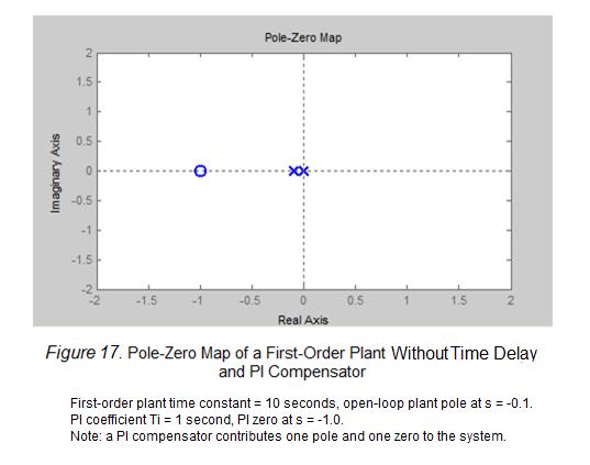
9 LIST OF FIGURES Figure 1 Open-Loop Response of a First-Order Plant Without Time Delay 2 Closed-Loop Response of a First-Order Plant Without Time Delay Page Open-Loop Response of a Pure Time-Delay Plant 5 4 Closed-Loop Response of a Pure Time-Delay Plant 6 5 Comparison of Approximated Time Delay and True Time- Delay Root Loci 8 6 Typical Feedback Loop With Time Delay 10 7 Constituents of PID Block 11 8 Pole-Zero Maps showing PI and PID Compensators in the S- Plane 9 Block Diagram Showing Proportional Compensation of a First-Order Plant Without Time Delay 10 Root Loci of First- and Second-Order Plants Without Time Delay Drawn by MATLAB 11 Root Loci of First- and Second-Order Plants Without Time Delay Drawn by the Numerical Algorithm 12 Block Diagram Showing Proportional Compensation of a First-Order Plant With Time Delay Root Loci of a First-Order Plant With Time Delay Block Diagram Showing Feedback Loop With Set-Point and Load-Disturbance Inputs 15 Root Loci, With Three Highlighted Test Points, for a First- Order Plant With Time Delay viii

10 16 Simulation of System Output for Highlighted Test Points in Loci 17 Pole-Zero Map of a First-Order Plant Without Time Delay and PI Compensator 18 Simulations of System Output for Three Test Points on the Root Loci Root Loci for Three Test Points of the PI Compensator Zero Simulations of System Output for Three PI-Zero Test Locations 21 Simulations of System Output for Three PI-Zero Test Locations with Overshoot Reduction Method Applied 22 S-Plane Map of a PID Compensator and Second-Order Plant Without Time Delay, and Resulting Root Loci 23 Root Loci of a PID-Compensated Second-Order Plant With Time Delay Performance of Recommended PID-Tuning Coefficients 54 C1 Impulse Responses for Pole Locations in the S-Plane 67 F1 Comparison of Padé Time-Delay Approximations 82 G1 Root Loci of a Pure Time-Delay Plant 87 G2 G3 Root Loci of a First-Order Plant With Time Delay Showing Marginal Gain Root Loci of a Single-Zero Plant, a Differentiator, With Time Delay G4 Root Loci of a Double-Zero Plant With Time Delay 98 G5 Root Loci of a Single-Pole, First-Order, Plant With Time Delay 99 G6 Root Loci of a Single-Pole, First-Order, Plant With Time 102 ix

11 G7 G8 H1 Delay (Close-up of Break-Away Point) Root Loci of a Double-Pole, Second-Order, Plant With Time Delay Root Loci of a PID-Compensated First-Order Plant With Time Delay Compensation Gain Giving 5% Overshoot for First-Order Plant With Time Delay I1 "Process Reaction Curve" 109 x

12 LIST OF TABLES Table 1 Recommended PI-Tuning Coefficients for a First-Order Plant With Time Delay 2 Comparison of the PID Double Zero Position That is the Basis for Tuning Recommendations to the Left-Most Position Where Loci Reenter the Real Axis 3 Recommended PID-Tuning Coefficients for a Second-Order Plant With Time Delay Page H1 Compensation Gain Yielding 5% Overshoot for a First-Order Plant With Time Delay 106 xi

13 1 1.0 Introduction In this study, a numerical method is developed for examining the paths of closedloop poles, root loci, in feedback systems with time delay. The paths of closed-loop poles are rarely tracked in these systems because of a mathematical difficulty posed by delay. The numerical method developed here not only averts this mathematical obstacle but enables recommendations to be made for PID-tuning coefficients in systems with time delay, which is also known as latency, transport delay, and dead time. For a pure dead-time process, whatever happens at the input is repeated at the output time units later (Deshpande & Ash, 1983, p. 10). In this research a novel application of root locus analysis is developed for producing tuning coefficients for proportional-integral (PI) and proportional-integralderivative (PID) compensators that give optimal transient response for first-order and second-order plants with time delay. The time response of a control system consists of two parts, the transient response and the steady-state response. By transient, we mean that which goes from the initial state to the final state (Ogata, 2002, p. 220). In this study, optimal transient response means rapid, and roughly equivalent, settling times after unit-step inputs in set-point change or load disturbance. Frequency response analysis assesses closed-loop system stability through openloop Bode and Nyquist plots (Stefani, Shahian, Savant, & Hostetter, 2002, p. 461), which convey the relationship of a plant's output at steady-state, in terms of magnitude and phase, to a sinusoidal input. Closed-loop pole analysis, on the other hand, characterizes

14 2 the nature of closed-loop dynamics by tracking closed-loop pole locations as a system parameter, typically compensation gain, is varied. The decay rate and oscillation frequency of each component of transient response, not easily predictable from timedelay Bode or Nyquist plots, are known once the location of the associated pole, or pair of poles, in the -plane is identified. The relationship between a pole's location in the plane and associated transient response is depicted in Figure C1. The transfer function of time delay is an exponential function of the complex variable, and delay (Ogata, 2002, p. 379). (1) The traditional symbol for angle is used because time delay introduces a phase angle difference between input and output sinusoids. The exponential transfer function, as we will see in Appendix G, leads to a system with time delay having a characteristic equation that is transcendental, meaning it can only be expressed by a function with an infinite number of terms. Since the conventional tool for drawing root loci, the MATLAB function rlocus(), cannot accommodate timedelay systems, another numerical technique is developed here (Appendix E). Root loci for systems with time delay can be constructed with several methods, for example, graphically (Ogata, 2002, p. 379), by approximating time delay (Vajta,

15 3 2000; Ogata, 2002), or by solving sets of simultaneous non-linear equations (Appendix E). Time-delay approximations, however, can lead to significant differences between predicted and actual responses. Such mismatches, as well as possible instabilities (see Figure 5; Silva, Datta, & Battacharyya, 2001), are avoided by drawing time-delay root loci with the straightforward and robust numerical technique developed in this study. Its predictions of closed-loop dynamic behavior and recommendations for PID coefficients are cross-checked against known results, MATLAB and SIMULINK simulations (Chapter 2), and mathematical derivations (Appendix G). The Problems With Time Delay Though a few systems actually benefit from the addition of time delay (Sipahi, Niculescu, Abdallah, & Michiels, 2011), time delay poses two difficulties to the control of simple plants of interest in this study: 1) it is inherently destabilizing, and 2) it is difficult to accommodate mathematically. Time delay's destabilizing influence is illustrated by comparing the output of a feedback system where the plant is pure time delay to a feedback system where the plant is first order. The open-loop response of a first-order plant is shown in Figure 1, where the plant time constant is 10 s. After a unit-step input, it settles to within 2% of final value after four time constants (40 s.)

16 4 The first-order plant can be accelerated with feedback. With a compensation gain of one, as shown in Figure 2, its output settles within 2% of final steady-state value in only 3.55 s. In Chapter 2 (Figures 10 and 11), it will be shown that the first-order plant s output is always accelerated by increasing compensation gain.

17 5 The open-loop response of a pure time-delay plant, on the other hand, is shown in Figure 3, where time delay is one second. When a feedback loop is comprised of a pure time-delay plant compensated at the same gain used for the first-order-plant in Figure 2, the system oscillates and never reaches steady state, as shown in Figure 4. Root loci drawn by the numerical algorithm (shown in Appendix G, Figure G1) are consistent with this time-series response. They show reducing compensation gain below one stabilizes the system, though it will remain oscillatory, and increasing compensation gain above one destabilizes the system. Loci cross the imaginary axis at a gain of one and at vertical positions. These positions correspond with angular frequencies, which exactly match the oscillating output, shown in Figure 4. Angular frequency, measured in, is 2 times frequency in time, which is measured in or Hz. Therefore, since 2, for an angular frequency of the associated

18 6 frequency in time is / 2 / 2 / 1 2. A frequency of 1/2 Hz corresponds with a period of 2 s, and clearly the period of oscillation in Figure 4 is 2 seconds.

19 7 The four simulations above show how time delay can have a destabilizing influence by isolating a pure first-order plant, and then a pure time delay plant, in a feedback loop. We saw the simple first-order plant is accelerated by feedback, but the pure time-delay plant oscillates and can become unstable. The difficulty that time delay poses to the mathematical analysis of feedback systems comes from its exponential transfer function, which leads to transcendental characteristic equations (explained in detail in Appendix G). Thus, is usually approximated by a rational polynomial. A comparison of root loci drawn by the numerical method in Figure 5 demonstrates the variations in predictions of system response that can be expected when using time-delay approximations. First-order Taylor and second-order Padé (see Appendix F; Ogata, 2002, p. 383) time-delay approximations are used to produce these root loci, which depict the closed-loop dynamics of compensated first-order and secondorder plants with time delay.

20 8 The compensation gain that puts closed-loop poles on the imaginary axis, marginal gain, places the feedback system in an oscillating state. Predictions of marginal gain by the three styles of time-delay approximations shown in Figure 5 clearly vary. The second-order Padé approximation is probably the most accurate, but still gives

21 9 optimistic predictions of marginal gain for the first-order plant and the PID-compensated second-order plant. A side effect of the numerical method is that loci appear wider than they actually are in some regions, and they become invisible in other regions. Loci path widths at a given location are easily thinned or broadened, however, by adjusting a parameter in the numerical algorithm, the decision criterion, as explained in Chapter 2 and Appendix E. Another way to draw time-delay root loci would be to seek roots of the closedloop characteristic equation by solving simultaneous non-linear equations. Real and imaginary parts of the characteristic equation would be the simultaneous equations of interest (Appendix E). The MATLAB function fsolve(), which requires an initial guess at the solution(s), could be used to find simultaneous solutions. Each call to fsolve() would return a value of that satisfies the closed-loop characteristic equation, and which would be a point on the loci. To completely define all branches comprising the loci throughout a region of interest in the s-plane, fsolve() must be called reiteratively with a variety of initial guesses at the solution to cover the region, and a variety of compensation gains to show response as a function of gain; some gaps might still be visible in the loci. The approach used in this paper offers a simpler implementation while identifying all points on the loci within a region of interest. The weakness of the numerical technique is that the widths of the loci can vary.

22 10 PID Compensation The PID compensator is a true workhorse of feedback control. The majority of control systems in the world are operated by PID controllers (Silva, Datta, & Battacharyya, 2002, p. 241). A typical application, control of a first-order plant with time delay, is shown in Figure 6. The simple proportional compensator, used in Figures 1 through 4, will mostly result in a static or steady-state error for plants of interest in this study, such as temperature-control loops (Astrom & Hagglund, 1995, p. 64; Ogata, 2002, p. 281). To eliminate steady-state error and accommodate higher-order plants, more complex PI and PID compensators must be used. As described in detail in Chapter 3, the integral (I) in PID eliminates steady-state error, and the derivative (D) improves transient response for high-ordered plants.

23 11 The PID compensator s transfer function is a summation of three terms; proportional, integral, and derivative, as shown in Figure 7. The proportional term produces control action equal to the product of process error, and compensation gain. The integral term produces control action equal to the continuous summation of process error times, an integral gain. Thus integral action can be expressed as a function of the complex variable.

24 12 The derivative term produces control action equal to the rate of change of the process times, a derivative coefficient. As will be seen in Chapter 3, the derivative stops ringing from occurring in a system composed of a proportionally-compensated second-order plant. The derivative term can be expressed as a function of. al., 2002). The complete PID transfer function is the sum of all three terms (Silva et, (2) The pole and two zeros of a PID compensator are easily identified by rearranging the three terms of over a common denominator. (3)

25 13 We see has a single pole that lies at the origin, where 0. The roots of its quadratic numerator 0 (4) are the two zeros of. When 0 in there is no derivative action, and the compensator has proportional and integral terms only. The transfer function of the PI compensator (5) has a pole at the origin, like the PID compensator, and a single zero. Setting 0 results in a proportional-only compensator, its transfer function is just gain, and it has no poles or zeros. (6) Review of PID-Tuning Approaches for Systems With Time Delay The process of selecting controller parameters to meet given performance specifications is known as controller tuning (Ogata, 2002, p. 682). A variety of theoretical approaches have been used to produce PID-tuning formulas for a first-order plant with time delay. A heuristic time-domain analysis (Hang, Astrom, & Ho, 1991) used set-point weighting to improve Ziegler and Nichols' (1942) original PID-tuning formulas, which were also determined empirically. Repeated optimizations using a third-order Padé

26 14 approximation of time delay produced tuning formulas for discrete values of normalized dead time" (Zhuang & Atherton, 1993, p.217). Barnes, Wang, and Cluett (1993) used open-loop frequency response to design PID controllers by finding the least-squares fit between the desired Nyquist curve and the actual curve. In reviews of the performance and robustness of both PI- and PID-tuning formulas, tuning algorithms optimized for setpoint change response were found to have a gain margin of around 6 db, and those that optimized for load disturbance had margins of around 3.5 db (Ho, Hang, & Zhou, 1995; Ho, Gan, Tay, & Ang, 1996). PID-tuning formulas were derived by identifying closed-loop pole positions on the imaginary axis, yielding the system s ultimate gain and period. Dynamics are said to suffer, however, for processes where time delay dominates due to the existence of many closed-loop poles near the imaginary axis, where the effect of zero addition by the derivative term is insignificant to change the response characteristics (Mann, Hu, and Gosine, 2001, p.255). In a general review of time-delay systems, Richard (2003) discusses finite dimensional models and robust H2 and H- methods. PID-Tuning Approach for Systems With Time Delay Used in This Study One outcome of this research is to recommend PI- and PID-tuning coefficients based on closed-loop pole analysis. PI coefficients for first-order plants and PID coefficients for second-order plants are given for six values of normalized time delay (NTD), the ratio of time delay to plant time constant. A two-step approach is used to generate the tuning coefficients for each plant type and NTD.

27 15 The first step is to select the most desirable locations for compensator zeros to lie. The rationale for selection of location is discussed in Chapter 3, in the sections on PI and PID-tuning of plants with time delay, where the effect of compensator zero locations on the form of loci is investigated, with three test points for the zeros. The location selection is also discussed in Appendix J, where an alternative mathematical method is used to show how zero locations affect break-away and reentry points. The ultimate goal of the zero-location selection criteria is to achieve the greatest net movement of closed-loop poles to the left. The second step is to draw the root loci and select the most desirable locations for the dominant closed-loop poles to lie on the loci. These locations determine compensation gain. The strategy of placing the compensator zero and choosing the point on the loci where closed-loop poles move farthest left seeks the fastest possible closed-loop transient response (see the depiction of the relationship of pole position to the nature of transient response time Figure C1). Under feedback, open-loop zeros attract closed-loop poles, so compensator zeros will be placed as far to the left as possible. In Chapter 3, it will be shown, using time delay limits, how far to the left a compensator zero can be placed before the plant s closed-loop poles no longer move toward it. Due to time delay, closed-loop poles get to the compensator zeros first. If compensator zeros are too far to the left, plant and

28 16 integrator poles move into the right half of the s-plane, which destabilizes the system, rather than moving to the left half of the s-plane, stabilizing and accelerating it. PI and PID compensators can be represented by mapping their poles and zeros in the s-plane as shown in Figure 8. For more details on mathematically identifying compensator poles and zeros, see Appendix D.

29 Validation of Numerical Algorithm In this chapter, the ability of the numerical method developed here to draw root loci for systems with time delay, is tested by comparing its output to known results for two simple plants without time delay. Proportional Compensation of First- and Second-Order Plants Without Time Delay A block diagram of a proportionally-compensated first-order plant without time delay is shown in Figure 9. Positions of this system's poles, closed-loop poles, are expressed as a function of below. Closed-loop pole paths are then plotted using MATLAB and the numerical method. Root-loci diagrams produced by the numerical method must match those drawn by MATLAB. The open-loop transfer function of the first-order system without time delay in Figure 9 is:

30 18 (7) Distefano, Stuberrud, and Williams (1995, p. 156) describe the canonical form of a system s closed-loop transfer function as: 1 (8) Thus, for the system in Figure 9, the closed-loop transfer function is The closed-loop characteristic equation of the system in Figure 9 is 1 0 (9) Values of that satisfy the closed-loop characteristic equation are its roots, they make the denominator of the closed-loop transfer function equal to zero so they are closed-loop poles. The characteristic equation of the system in Figure 9 is 0 (10)

31 19 If the plant is time invariant, the open-loop pole is constant, so the position of the closed-loop pole is simple to express as a function of. (11) If the plant in Figure 9 is second-order, for example, having poles at 0.1 and 1.0, the open-loop transfer function is: (12) The closed-loop transfer function is: 1 (13) Closed-loop pole locations for this second-order system are the roots of its characteristic equation: 0 (14) Roots of this second-order equation, as well as higher-order equations, can be found with the MATLAB function roots(), which takes polynomial coefficients as input and returns roots

32 20 >>roots([1 p1+p2 p1*p2+kp]) The MATLAB function rlocus() takes the uncompensated open-loop system transfer function as input, as described by polynomial coefficients, plots the positions of closed-loop poles, root loci, as varies from zero to infinity It does this by iteratively varying, and at each value finding the roots of the closed-loop characteristic equation, then plotting them. Root loci for the closed-loop system shown in Figure 9, which contains a firstorder plant with a pole at 0.1, would be drawn by issuing the MATLAB command: >> rlocus([1], [1 0.1]) If the closed-loop system contains a second-order plant, for example with poles at 0.1 and 1.0, root loci would be drawn with the MATLAB command: >> rlocus([1], [ ]) These two calls to rlocus() generated the two root-loci plots in Figure 10.

33 21 To validate the numerical algorithm, which will be used mostly for systems with time delay, the root loci that it draws for systems without time delay will be compared to the root loci drawn by MATLAB in Figure 10. Loci drawn by the numerical algorithm are shown in Figure 11. Note they differ from the MATLAB plots in that they are shaded and the widths of loci vary. The match between the depictions of closed-loop pole trajectories in Figures 10 and 11, however, is close enough to validate the tool. Further details are discussed in Appendix E.

34 22 Systems with time delay have transcendental closed-loop characteristic equations, so the rules of root locus construction need to be modified (Ogata, 2002, p. 380). The MATLAB function rlocus() cannot draw root loci for such systems because their characteristic equations are transcendental (described in Appendix E). Another option for drawing time-delay root loci would be to use the MATLAB function fsolve() which finds roots of non-linear equations. In addition to a description of the non-linear equation it

35 23 requires an initial guess at the solution as input. Each point in a dense grid of points covering a region of interest in the s-plane would need to be input, and for a wide variety of gains. This method could still leave gaps in the loci. The method used in this paper, however, is favored for its simplicity and robustness. It analyzes the angle and magnitude conditions of the closed-loop characteristic equation, and is equally effective whether the equation is of polynomial form or transcendental. The first step is to evaluate the angle condition of the characteristic equation. For the system in Figure 9, the characteristic equation is 1 0 This equation is a function of the complex variable so each side of the equation has a magnitude and phase angle. After moving the one to the right-hand side the phase angle component of each side is expressed ,1,2, (15) Closed-loop pole positions are identified by computing A at each point on a grid that spans a region of interest in the s-plane. Locations where the angle condition is satisfied to within a specific criterion 180 are marked as being on the loci, though their proximity to the actual

36 24 loci depends on the decision criterion. Locations may be right on or just very close to the root locus. Compensation gains at the pole locations are computed from the magnitude condition which comes from taking the magnitude of each side of the characteristic equation, for the system in Figure 9 this gives 1 1 Compensation gain at each pole location is then 1 and is conveyed through color coding in the plots. For this study, the decision criterion remains constant throughout any given plot, but varies from plot to plot as appropriate, to keep loci as thin as possible. The reason loci widths vary within a given plot is because the rate of change of is a function of, yet the decision criterion remains constant. As a result, some points that are not actual roots look like they are roots because they get color coded. Figure 10 (drawn by MATLAB) and Figure 11 (drawn by the numerical method developed in this paper) are essentially equivalent depictions of closed-loop system transient response, and so they serve as partial validation of the numerical method. Both depictions show the first-order plant s return to steady state after a transient input is

37 25 accelerated with feedback, simply by increasing compensation gain. As increases from zero to infinity, the single closed-loop pole in the system follows a perfectly straight path from the open-loop pole position 0.1 to its final destination, (Figure C1 depicts the relationship between a pole's position, and its resulting impulse response, with an s-plane map of impulse response versus pole location throughout a region surrounding the origin). The second-order plant s return to steady state after a transient input, on the other hand, is accelerated to a certain point by increasing compensation gain, but then the system starts to ring if increases past that point, as shown in Figures 10 and 11. The plot of the second-order plant in both figures shows two open-loop poles that lie on the real axis. As increases, they approach each other and collide; after colliding the poles depart the real axis in opposite directions. Up to the point when both poles collide, increasing gain accelerates the system. Beyond that point, increasing gain will not accelerate the system, and merely leads to ringing at ever higher frequencies.

38 Results In this chapter, the numerical technique will draw root loci for systems with time delay, and then produce PI- and PID-tuning recommendations for first- and second-order plants with time delay. The method of drawing root loci will be demonstrated on feedback systems without time delay, and then time delay will be brought into the loop. PI-tuning coefficients will be stated for a first-order plant with time delay, and PID-tuning coefficients will be stated for a second-order plant with time delay, for six values of normalized time delay (NTD), the ratio of time delay to plant time constant. Proportional Compensation of a First-Order Plant With Time Delay Next, the numerical method draws root loci for the time-delayed system in Figure 12, a proportionally-compensated first-order plant with time delay. Root loci of this system are depicted at two magnification levels in Figure 13. Note the two highlighted locations on the loci, they are complex conjugates and

39 27 correspond with a compensation gain 4.8. These pole locations are 45 from the real axis and, in a purely second-order system, would correlate with a damping coefficient 0.7, meaning, during recovery from a transient input, the overshoot of the final value is expected to be 5% (Ogata, 1970, p. 238). By comparing Figure 13 to Figures 10 and 11, we see the difference between the closed-loop dynamics of a first-order plant with time delay and a first-order plant without

40 28 time delay. The loci in Figure 13 are consistent with the assertion, proven in Appendix G, that time delay introduces an infinite set of loci to the system. The three loci trajectories shown in Figure 13 are members of that infinite set. Two closed-loop poles due to time delay define loci that run from left to right, roughly parallel but slightly away from the real axis. A third pole due to delay forms a locus with the plant pole. The timedelay pole starts from and travels to the right along the real axis as gain increases, it eventually collides with the plant pole, which moves left from its open-loop position. For this system, as shown in Appendix G (Equation G12), the compensation gain associated with a closed-loop pole crossing the imaginary axis is nearly proportional to the pole's distance from the real axis : 1 G12 A system is marginally stable when a closed-loop pole crosses the imaginary axis and no other poles are in the right-half side of the -plane. Thus, according to the equation above, in a first-order system with time delay closed-loop poles that are closest to the real axis are dominant. If the system is purely second order without time delay, applying the gain that places closed-loop poles at the positions highlighted in Figure 13 would result in a 5% overshoot of the final value after a transient input (Distefano et al., 1995, p. 98). However, even though the plant is really first order with time delay, we will see shortly SIMULINK simulations (Figure 16) show its behavior mimics a higher-order plant without time delay. Based on this observation, recommendations for compensation gain,

41 29 stated in Appendix H for a first-order plant with time delay, are produced by putting the dominant closed-loop poles at these locations. All tuning recommendations put forth in this paper are evaluated by measuring the overshoot of final value produced, as well as the time required for the process to settle within 2% of final value, 2% settling time, after unit-step changes in set point and load disturbance. As shown in Figure 14, the load disturbance is introduced immediately downstream of the compensator. Three separate compensation gains, associated with the three highlighted closedloop pole positions in Figure 15, are used for simulating system output. The three highlighted points correspond with compensation gains of 3.3, 4.9, and In a purely second-order system, poles at the angular positions, with respect to the origin,

42 30 shown in Figure 15, would correlate with damping coefficients of = 1.0, 0.707, and nearly 0.0, respectively (Distefano et al., 1995, p. 98).

43 31 The three SIMULINK simulations in Figure 16 show system response after unitstep changes in set point and load disturbance for the three compensation gains associated with the highlighted pole locations in Figure 15. The time-series response in Figure 16 suggests the dynamic behavior of a first-order plant with time delay is similar to the dynamic behavior of a higher-order plant without time delay. At low gains there is no ringing, at medium gains there is some ringing, and at high gains there is plenty of ringing. Note, in this system, the final steady-state value is not guaranteed to match set point, however, system output happens to reach the desired value because, after the unitstep load disturbance, the input to the plant is exactly the desired output, so once the control output goes to zero the plant output will equal the desired value.

44 32 Test Point 1: 3.3. Closed-loop pole positions are on the real axis and have no imaginary component. As expected, the system's output is free of oscillations. Test Point 2: 4.9. Closed-loop pole positions are 45 from the real axis and would correspond with 5% overshoot in a purely second-order system. Actual overshoot of final steady-state value is about 5%. Test Point 3: 12. Closed-loop pole positions are close to the imaginary axis. The system is stable, but it is near marginal stability.

45 33 Recommendations for compensation gain, for control of a first-order plant with time delay, are tabulated in Appendix H for seven values of normalized time delay (NTD) covering the range System performance, as measured by 2% settling time after a unit-step change in set point or load disturbance, resulting from the recommended gains is also tabulated. Overshoot, verified through SIMULINK simulations, are within 5%. Recommendations are based on root-loci diagrams, like the one shown in Figure 15, created for each value of NTD. Proportional-Integral (PI) Compensation of a First-Order Plant Without Time Delay In the previous example, where a first-order plant is proportionally compensated, steady-state error is apparent (see Figure 16). Steady-state error can be eliminated, however, if a factor of, an integrator, exists in the open-loop transfer function (Ogata, 2002, p. 847). When integral control action is added to a proportional compensator a proportional-integral (PI) compensator is created. Its transfer function is the sum of proportional and integral terms: (16) The pole of lies at the origin 0, its zero lies at.

46 34 Compensation gain is common to both proportional and integral terms when the integral term is expressed as, where is integral time (Astrom & Hagglund, 1988, p. 4): (17) The zero of is then independent of and lies at. This form of simplifies our analysis because the zero location is determined by a single parameter, and values of proportional gain are read directly from the root locus diagram and its associated closed-loop pole position immediately identified. Proportional-Integral (PI) Tuning Strategy With and Without Time Delay The strategy for tuning plants with time delay is now introduced and applied to plants both with and without time delay. Since a PI compensator s pole must lie at the origin of the s-plane, but its zero can be placed anywhere on the real axis at the discretion of the designer, the compensator is tuned by first placing its zero, then drawing root loci, and finally choosing compensation gain so closed-loop poles are at the most desirable location. This sequence will now be described.

47 35 Placement of PI zero. In determining the best place to put the PI zero, we consider two rules restricting movement of closed-loop poles in the s-plane: Under feedback, as compensation gain increases from zero to infinity, the root locus branches start from the open-loop poles and terminate at zeros (Ogata, 2002, p. 352). Zeros remain fixed in place. If the total number of real poles and real zeros to the right of a test point on the real axis is odd, then that point is on a locus (Ogata, 2002, p. 352). To meet the goal of accelerating the plant beyond its open-loop response, by pulling open-loop poles to the left, the PI zero is placed to the left of the plant pole, as shown in Figure 17. In this configuration the two portions of the real axis that will contain loci, according to the second rule stated above, lie between the two open-loop poles and to the left of the PI zero. It will be shown that only in systems without time delay can open-loop plant and integrator poles be pulled to the left of the PI zero, regardless of how far to the left the PID zero is placed. In such systems, transient response can always be accelerated simply by increasing compensation gain.

48 36

49 37 Drawing root loci. Root loci are next drawn by the numerical algorithm for the open-loop system without time delay depicted in Figure 17. Loci for this system are shown in Figure 18 where, as increases from 0 to 70, the two open-loop poles approach each other on the real axis and collide. Both poles then depart the real axis and head left to reenter the real axis on the left side of the PI zero. The numerical algorithm s drawing agrees with well-known behavior and shows the general shape of loci that can be expected for this type of system, regardless of how far to the left the PI zero is placed.

50 38 Three SIMULINK simulations show system output for three different PI compensators, where 1 second. Three compensation gains, 18, 38, and 51, complete the design of the three PI controllers, and are associated with the three closedloop pole locations highlighted in Figure 18. The simulations show the closed-loop system returns rapidly to steady state after unit-step changes in set point or load

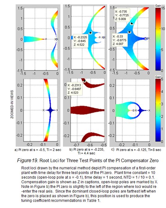
51 39 disturbance and two percent settling times are much shorter than in open-loop. Such performance is consistent with the fact that closed-loop poles are relatively far to the left of the open-loop plant pole. Choosing compensation gain. Once loci are drawn, the compensation gain that results in the most desirable closed-loop pole locations, in terms of system performance, can be chosen. For example, to favor a heavily-damped response closed-loop poles should be close to or on the real axis. To favor less damping, which in some cases leads to faster response (such as in a purely second-order system), closed-loop poles should be off the real axis, but no more than 45 from the real axis. Proportional-Integral (PI) Compensation of a First-Order Plant With Time Delay When time delay is introduced to the feedback system previously discussed, a PIcompensated first-order plant, the compensator s zero can no longer be placed anywhere along the real axis and still pull open-loop plant and integrator poles over to its left side. Instead, if the PI zero is placed too far to the left of the origin, a closed-loop pole due to time delay gets to it first. Plant and integrator poles are forced to head into the right-half plane. Root loci produced by the numerical tool are drawn at two different levels of scale in Figure 19, using three test points for the PI zero. The three test points are located relatively far to the left ( 0.5, just barely to the left ( 0.235, and to the right ( 0.1 of the left-most part of the region that allows open-loop plant and integrator poles to reenter the real axis.

52 40

53 41 The connection between the three highlighted closed-loop pole positions in Figure 19, which define three different PI compensators, and associated time responses of the system, is made in Figure 20. System output after unit-step changes in set point and load disturbance is simulated for each controller.

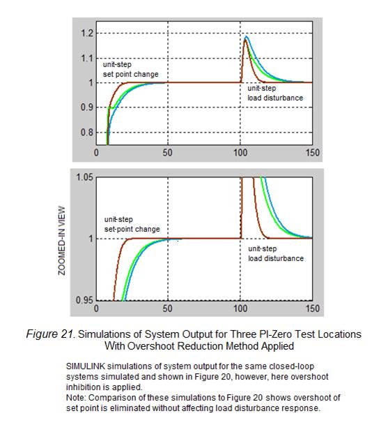
54 42 This study found that closed-loop poles move farthest to the left when the PI compensator zero is placed slightly to the left of the location that allows loci to reenter the real axis (see Figure 19b). As measured by 2% settling time, this zero position gives the fastest recovery after a load disturbance (see Figure 20). During recovery to steady state after a set-point change, however, there is too much overshoot. Overshoot of set point can be eliminated, however, with a technique that leaves load-disturbance response unaltered, as shown in Figure 21 where system output is simulated for the same compensators used in Figure 20, but each compensator is modified to implement this overshoot reduction method. The overshoot-reduction technique used here linearly decreases the natural rate of integration as the distance between set point and process value grows. Effective integration rate drops to zero when the process is separated from set point by one proportional band = 1/.

55 43

56 44 Proportional-Integral (PI) Coefficients for a First-Order Plant With Time Delay Recommendations for PI-tuning parameter sets and, are given in Table 1 for six values of NTD; each set of coefficients is generated for a given NTD, from a rootlocus plot similar in form to the one shown in Figure 19b. The design goal is to move closed-loop poles as far to the left of the PI zero as possible.

57 45 Table 1 Recommended PI-Tuning Coefficients for a First-Order Plant with Time Delay. NTD Recommendation Result Recommendation Result Result PI-Zero Position (Multiples of Open-Loop Plant Pole Position) Equivalent Ti (% of Open-Loop Plant Time Constant) 2% Settling Time Unit- Step Change in Set Point (Multiples of Open- Loop Plant Time Constant) 2% Settling Time Unit- Step Change in Load Disturbance (Multiples of Open- Loop Plant Time Constant) These recommendations meet the design goal of short settling times after unit-step changes in set point and load disturbance that are roughly equivalent when the PI compensator is modified to eliminate overshoot of set point as described in the text. Note shortest settling times occur with smallest normalized time delay, NTD.

58 46 Proportional-Integral-Derivative (PID) Compensation of a Second-Order Plant Without Time Delay A closed-loop feedback system, comprising a second-order plant without time delay, will ring or oscillate at high gains, as previously discussed and depicted with root loci in Figures 10 and 11. Ringing can be eliminated, however, by adding derivative action to the compensator, which adds another zero to the system (see Chapter 1: PID Compensation and Appendix D). Derivative action allows higher gains to be used on a second-order plant without time delay because it suppresses ringing at high gains, as illustrated by the root loci in Figure 22 where two closed-loop poles depart the real axis but reconnect with it to the left of the PID double zero. Loci will reconnect with the real axis to the left of the compensator double zero, regardless of how far to the left the double zero is placed.

59 47 PID tuning recommendations will put both PID zeros at the same location, making a double zero because this maximizes their ability to pull closed-loop poles to the left.

60 48 Proportional-Integral-Derivative (PID) Compensation of a Second-Order Plant With Time Delay When one or two time constants dominate (are much larger than the rest), as is common in many processes, all the smaller time constants work together to produce a lag that very much resembles pure dead time (Deshpande & Ash, 1981, p. 13). Such a process can be described by a three-parameter double-pole second-order plant model and time delay (Astrom & Hagglund, 1995, p. 19): (18) Recommendations for PID-tuning coefficients will be based on this plant model.

61 49 Proportional-Integral-Derivative (PID) Coefficients for a Second-Order Plant With Time Delay Recommendations for PID-tuning coefficients are based on root-loci diagrams drawn by the numerical tool, which are similar in form to those used for PI-compensator design (Figure 19), and SIMULINK simulations for verification. Figure 23 depicts the dynamic behavior of a second-order plant, modeled by a double pole at 0.10, with a two-second time delay. The plant is controlled by a PID compensator with a double zero at The double zero is slightly to the left of the region which allows closed-loop poles to reenter the real axis. After colliding and departing the real axis, open-loop plant and integrator poles move to the left, roughly parallel to the real axis as gain continues to increase, before moving away from the real axis and back toward the right-half plane. As was the case for PI-tuning of a first-order plant with time delay, PIDtuning recommendations are generated from root loci with this form because, for a limited range in compensation gain, closed-loop poles move relatively far to the left of their open-loop positions.

62 50 For a given second-order plant, the left-most point on the real axis that the PID double zero can be placed, and still draw plant and integrator poles to its left to reenter the real axis, is forced to the right as time delay increases. The relationship between NTD and the maximum distance of separation between the double zero and the open-loop double pole is shown in Table 2. When 0.5 the double zero can no longer be placed far enough to the left of the plant's open-loop double pole to allow for reasonable

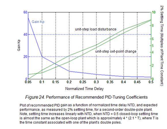
63 51 error in modeling the plant, so PID-tuning recommendations are stated in Table 3 only for the range Two transient response performance metrics, overshoot and 2% settling time, for the tuning coefficients are stated in Table 3 and plotted as a function of NTD in Figure 24.

64 52 Table 2 Comparison of the PID Double Zero Position That is the Basis for Tuning Coefficient Recommendations to the Left-Most Position Where Loci Reenter the Real Axis Finding Recommendation NTD Leftmost position on the real axis the PID double zero can be placed, where plant poles will reenter the real axis (multiples of plant double pole open-loop position) Position of the PID double zero selected for determining tuning coefficients (multiples of plant double pole open-loop position) Comparison between two key locations of the PID double: 1) the left-most position on the real axis that permits plant poles to reenter the real axis, and 2) the position used to produce tuning coefficients. Choice of the position for coefficients (listed in Table 3) is based on root loci drawn by the numerical algorithm, matching the form shown in Figure 23. For each value of NTD, SIMULINK simulations were created to verify the design goal is achieved. The goal is rapid return to steady-state conditions, after unitstep changes in set point or load disturbance, by achieving net movement of closed-loop poles to the left. Note: the left-most position the double-zero can be placed and still allow loci to reenter the real axis, moves to the right, toward the open-loop plant double pole, as normalized time delay NTD increases. This effect conveys deterioration in the ability of a PID feedback loop to accelerate the plant as NTD increases

65 53 Table 3 Recommended PID-Tuning Coefficients for a Second-Order Plant with Time Delay NTD Recommendation Finding Recommendation Finding Finding PID double-zero position (multiples of plant double pole open-loop position) Equivalent Ti, Td (multiples of one of the plant's double poles' time constant) 2% settling time after a unit-step change in set point (multiples of one of the plant's double poles' time constant) 2% settling time after a unit-step change in load disturbance (multiples of one of the plant's double poles' time constant) , , , , , , Recommendations for PID-tuning coefficients, and in control of a second-order plant with time delay. Coefficients meet the design goal of rapid, and roughly equivalent 2% settling times, after a unitstep change in set point or load disturbance. Simulations of system response used to generate these settling times used the suggested method of reducing set point overshoot described in the text. Note shortest settling times occur with small NTD.

66 54

67 55 PID coefficient recommendations for optimal load-disturbance response have been found to vary from those giving optimal set-point change response (Zhuang & Atherton, 1993). The tuning recommendations given here optimize both set-point change and load-disturbance settling times, though they intrinsically favor load disturbance and lead to overshoot after a set-point change, by applying an overshoot-reduction method. The natural rate of integration called for by the PID algorithm's integral term is linearly reduced as the distance between set point and process value grows, such that the integration rate reduces to zero when: 1 After modifying the PID algorithm with this overshoot-reduction technique, PIDtuning coefficients shown in Table 3, will give rapid and roughly equivalent settling times after a unit-step change in set point or load disturbance, and with no overshoot.

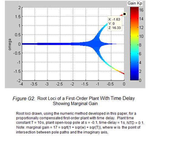
68 Conclusion Root loci for systems with a variety of polynomial transfer functions are commonly drawn and discussed in textbooks on classical control theory. However, pure polynomial transfer functions cannot exactly express the effect of time delay. Time delay is prevalent in control systems, so it is of interest to see what loci for time-delay systems actually look like. In this study, a comprehensive set of root loci for these systems is exhibited and then used to design PID compensators for first-order and second-order plants with time delay. Root loci for plants with time delay are drawn by a numerical method developed here. The method avoids the need to approximate time delay and the mismatch between predicted and actual response that sometimes results (see Figure 5). The methodology used here shows: How to identify the true positions of closed-loop poles in feedback systems with time delay. How to identify marginal gain (Figure G2) in feedback systems with time delay. Predictions of the numerical method developed here are consistent with mathematical analysis and show: In feedback systems with time delay an infinite number of separate and distinct closed-loop pole trajectories will exist. As compensation gain increases from zero, closed-loop poles follow paths that start at the far left

69 57 extreme of the real axis, separated vertically by a distance of where is time delay, and travel to the right, roughly parallel with the real axis. Some time-delay poles may be consumed by plant zeros, or system poles my be contributed, but ultimately an infinite number of closed-loop poles trend along horizontal asymptotes as gain increases, toward the right extreme of the real axis, at vertical positions 2 1 where 0, 1,2, (see Appendix G, Figure G7). In a first-order system with time delay, the two closed-loop poles that cross the imaginary axis closest to the real axis are dominant because they are the first poles to cross into the right-half plane (Appendix G and Figure 13). The behavior of a first-order plant with time delay is similar to the behavior of a higher-order plant without time delay. As shown in Figure 16, the first-order plant with time delay begins to ring as compensation gain increases. An explanation is given for the limitation in the ability of PI and PID controllers to effectively accelerate open-loop transient response, as NTD increases. There is a restriction on how far to the left of origin a compensator zero can be placed, so that closed-loop poles travel to its left and accelerate the system (see Appendices I and J). As shown in Figure

70 58 23, a pole due time delay gets to the compensator zero first, so plant and integrator poles must move into the right half of the -plane. The culmination of this research is the generation of PI-tuning coefficients for first-order plants with time delay, and PID-tuning coefficients for second-order plants with time delay. Coefficients are stated for a range in normalized time delay of When used with a modification that reduces overshoot of the final value after a set-point change, these coefficients give rapid return to within 2% of steady state after a unit-step change in set point or load disturbance.

71 59 References Arfken, G. (1970). Mathematical methods for physicists (2nd ed.). London: Academic Press. Astrom, K. J., & Hagglund, T. (1988). Automatic tuning of PID controllers. Research Triangle Park, NC: Instrument Society of America. Astrom, K. J., & Hagglund, T. (1995). PID controllers: Theory, design, and tuning (2nd ed.). Research Triangle Park, NC: Instrument Society of America. Barnes, T. J. D., Wang, L., & Cluett, W. R. (1993, June). A frequency domain design method for PID controllers. Proceeding of the American Control Conference, San Francisco, Beyer, W. H. (Ed.). (1981). Standard mathematical tables. Boca Raton, FL: CRC Press. Deshpande, P. D., & Ash, R. H. (1981). Elements of computer process control with advanced applications. Research Triangle Park, NC: Instrument Society of America. Distefano, J. J., Stuberrud, A. R., & Williams, I. J. (1995). Feedback and control systems (2nd ed.). United States of: McGraw-Hill. Hang, C. C., Astrom, K. J., & Ho, W. K. (1991). Refinement of the Ziegler-Nichols tuning formula. IEE Proceedings, 138(2), Ho, W. K., Gan, O. P., Tay, E. B., & Ang, E. L. (1996). Performance and gain and phase margin of well-known PID tuning forumlas. IEEE Transactions on Control Systems Technology, 4(4),

72 60 Ho, W. K., Hang, C. C., & Zhou, J. H. (1995). Performance and gain and phase margin of well-known PI tuning forumlas. IEEE Transactions on Control Systems Technology, 3(2), Mann, G. K. I., Hu, B. -G., & Gosine, R. G. (2001). Time-domain based design and analysis of new PID tuning rules. IEE Proceedings-Applied Control Theory, 148(3), Ogata, K. (1970). Modern control engineering. Englewood Cliffs, NJ: Prentice Hall. Ogata, K. (2002). Modern control engineering (4th ed.). Englewood Cliffs, NJ: Prentice Hall. Richard, J-T. (2003). Time-delay systems: an overview of some recent advances and open problems. Automatica, 39, Silva, J. S., Datta, A., & Battacharyya, S. P. (2001). Controller design via Pade approximation can lead to instability. Proceedings of the 40 th IEEE Conference on Decision and Control, Silva,J. S., Datta, A., & Battacharyya, S. P. (2002). New results on the synthesis of PID controllers. IEEE Transactions on Automatic Control, 47(2), Sipahi, R., Niculescu, S., Abdallah, C., & Michiels, W. (2011). Stability and stabilization of systems with time delay: limitations and opportunities. IEEE Control Systems Magazine, 31(1), Stefani, R. T., Shahian, B., Savant, C. J., & Hostetter, G. H. (2002). Design of feedback systems. New York, NY: Oxford University Press.

73 61 Vajta, M. (2000). Some remarks on Padé-approximations. 3rd Tempus-Intcom Symposium, Vezprem, Hungary, 1 6. Valkenburg, M. E. (1964). Network analysis (2nd ed.). Englewood Cliffs, NJ: Prentice Hall. Zhuang, M., & Atherton, D. P. (1993, May). Automatic tuning of optimum PID controllers. IEE Proceedings-D, 140(3), Ziegler, J. G., & Nichols, N. B. (1942). Optimum settings for automatic controllers. Transactions of the ASME,

74 62 Appendices Appendix A Laplace Transform The Laplace integral transform simplifies the process of solving ordinary differential equations, which describe the physical systems, or plants, we want to control. Timebased differential equations are converted to polynomial functions of the complex variable, simplifying analysis of feedback dynamics. A function in time is transformed to a function of (Arfken, 1970, p. 688) lim (A1) Consider a simple, first-order plant, its time response to an impulse input will exponentially decay, with time constant (A2) The Laplace transform of the plant, its transfer function, is 1 1 The plant transfer function has a pole, goes to infinity, at.

75 63 Appendix B Inverse Laplace Transform and Residue Theorem When the Laplace Transform is applied in characterizing the dynamic behavior of a feedback system, the ability to convert back to the time domain is eventually needed. Transformation of a function of a complex variable,, into a function of time,, is accomplished with the Inverse Laplace Transform (McCollum 1965) (B1) The contour integral must surround a region in the plane that contains all the poles of. The residue theorem from complex analysis helps us apply the Inverse Laplace Transform. Residues of a polynomial, are the coefficients in its Laurent expansion, they will be calculated below through partial fraction expansion. The residue theorem 2, (B2) states the sum of residues within an encircled region is proportional by 2 to the contour integral around the region. As an example, the time-domain response is determined for a first-order plant, with transfer function, excited by a unit-step input 1.

76 64 function The output of the plant is the product of its input and the plant transfer (B3) Using the residue theorem, the Inverse Laplace Transform is computed as the sum of the residues of lim lim 1 (B4)

77 65 Appendix C Tools Frequency analysis. In steady-state frequency analysis, a plant is excited by a sinusoidal signal with a constant frequency and magnitude. After a transient period elapses the system output will oscillate at steady-state and, if the system is linear, it oscillates at the same frequency as the input signal. A difference between the phase and magnitude of the input and output signals, however, will probably be present. The manner in which the plant alters the phase and magnitude of the input signal, as a function of frequency, is an indication of the plant's stability in a closed-loop system. Stability can be determined from gain and phase margins (Ogata, 1970, p. 430) and from the phase crossover frequency (Stefani et al., 2002, p. 465), the frequency at which input and output sinusoids are out of phase. Gain margin is the ratio of the magnitudes of input and output signals at. If gain margin is greater than one the system is stable, when it's equal to one the system will continuously oscillate, being marginally stable. When gain margin is less than one the system is unstable. Phase margin is the amount of additional phase lag at the crossover frequency required to bring the system to the verge of instability (Ogata, 2002, p. 562). In systems that are not second order phase and gain margins give only rough estimates of the effective damping ratio of the closed-loop system (Ibid, p. 565).

78 66 The introduction of time delay affects only the phase of the output signal, its magnitude remains unchanged. The transfer function of time-delay (Equation 1) at steady-state, 0, is, where is time delay. Thus, time delay adds a phase lag of, a value which increases with frequency and the actual time delay, as compared to the delay-free system.

79 67 S-plane analysis. The transient response of a linear system is comprised by one or more first- or second-order response components that, in a stable system, decay exponentially. Any first- or second-order response can be correlated with a single pole or pair of poles, respectively, in the s-plane as shown below in Figure C1. Plant poles that lie off the real axis must occur in complex conjugate pairs for the plant transfer function coefficients to be real.

80 68 Impulse responses of first- and second-order plants are shown in Figure C1; this visual aid describes the type of time-response that can be expected for a pole s location in the s-plane. Total transient response is the sum of all individual time-responses in a system (Valkenburg, 1964, pp ). Given a polynomial expression for total system output, the amplitude of each component of response is determined through partial fraction expansion of. The following rules summarize the relationship between impulse response and pole positions in s-plane shown in Figure C1 Poles in the left half of the s-plane represent stable response Poles on the real axis indicate the absence of oscillatory content Poles off the real axis indicate the presence of oscillatory content.

81 69 Comparison of closed-loop pole analysis to frequency analysis. Closed-loop pole analysis can produce root loci which show the movement of closed-loop poles, and thus describe the dynamic behavior of a plant in feedback, as a parameter, typically compensation gain, varies. Steady-state frequency analysis assesses closed-loop stability by examining the open-loop plant and how it transforms a sinusoidal input to the resulting sinusoidal output, as a function of frequency. The two techniques intersect along the imaginary axis in the s-plane where and. Poles that lie on this axis represent impulse responses that are continuous oscillations (Stefani et al., 2002, p. 465). In root-locus analysis, if a pole is on the imaginary axis and no poles are in the right half of the -plane, the system output continuously oscillates. The compensation gain associated with this pole position is the reciprocal of what s referred to as gain margin in frequency analysis. The vertical position of the pole on the imaginary axis is the phase cross-over frequency, the frequency of excitation at which input and output sinusoids are 180 out of phase.

82 70 Appendix D Identifying the Poles and Zeros of a PID Compensator The method of using root locus in this paper for tuning PID controllers makes proportional gain a common factor to all three PID terms by expressing the integral term as, where is integral time, and the derivative term as where is derivative time (Astrom & Hagglund, 1995, p. 6) (D1) A PI compensator s zero location then depends only on, a PID compensator s two zeros locations, identified below with the quadratic equation, depend only on and. 1 (D2)

83 71 Imaginary zeros. Both PID compensator zeros lie off the real axis when the argument of the square root term in Equation D2 is negative because the square root, and PID zeros, will have imaginary components. The argument of the square root term is 1 4 which is less than zero when 4 Real zeros. Both PID compensator zeros lie on the real axis when the argument of the square root term is greater to or equal to zero or 4 (D3) Both zeros lie at the same position, a repeated or double zero, when the argument of the square root term equals zero; this occurs when 4 (D4) This ratio of to is recommended in Ziegler-Nichols tuning forumlas (Ziegler & Nichols, 1942).

84 72 As becomes very large compared to, the pole-zero configuration of a PID compensator approaches that of a PI-only compensator. Expansion of the expression for zero positions resulting from applying the quadratic equation above 1 (D5) Applying the binomial series expansion (Beyer, CRC Standard Mathematical Tables, 1981, p. 347) gives 1!! (D6) If, higher-order terms vanish 1 0 (D7) or, (D8)

85 73 Appendix E Numerical Computation of Root Locus With and Without Time Delay The numerical method developed in this paper finds poles of feedback systems with time delay by brute-force. The roots of the systems' transcendental equation are found by calculating the value of the open-loop transfer function at each point on a grid of finely spaced points within a region of interest in the plane. For example, consider the closed-loop characteristic equation of a proportionally- compensated plant with time delay 1 0 (E1) where compensation gain is. Values of that represent positions of poles in the plane satisfy the characteristic equation's angle condition 1 (E2) By recognizing that any angle equals 2 it is clear how the exponential component contributes an infinite number of poles to the system 2, 0,1,2 (E3)

86 74 The value of is computed at each point on a\the grid, locations where this value is within a small range of 180, the decision criterion or as labeled in the code phase variation, are considered to be on the loci. The characteristic equation's magnitude condition is 1 1 (E4) It gives the value of compensation gain at any location on the loci (E5) The open-loop transfer function of a PI compensated first-order plant with time delay can be written (E6) where is integral time and is the plant time constant. An excerpt from MATLAB code developed in this study shows the open-loop transfer function written as

87 75 G = exp(-s*timedelay)*(1/(timeconst*s+1))*(((s+tizero))/s); The value of G is calculated at all points on the grid in the region of interest. Locations where is within a specified range around 180 are stored for plotting, they form the loci. if ( (thephase > (180 - phasevariation)) & (thephase < (180 + phasevariation)) ) Each point is color-coded to match the value of compensation gain which is calculated from the magnitude condition K = 1 / abs(g); Root loci are depicted by plotting the magnitude of throughout the region of interest in the s-plane which has boundaries at,,, and. surf(omegamin:omegaincrement:omegamax, sigmamin:sigmaincrement:sigmamax, abs(k)); The open-loop transfer function of a PID compensated second-order plant with time delay can be expressed

88 76 (E7) This form clearly shows the open-loop transfer function's two poles and two zeros. Note is a common factor to all terms. In MATLAB code the open-loop transfer function is written GH = exp(-s * TimeDelay) * (1/((TimeConst1 s + 1) ) *(1 / (TimeConst2 s + 1)) * ((s + tizero) * (s + tdzero)) / s; criterion. Points on the loci are again identified by the angle condition and the decision 1 Then compensation gain at each point on the loci is found from the magnitude of GH 1 / abs(gh) The derivative time is extracted from this quotient as follows to get compensation gain kp(sigmacounter, omegacounter) = (tizero + tdzero)*1/abs(gh);

89 77 because (E8) An alternate method of finding roots of transcendental equations. An alternative to the technique developed in this paper would be to use the MATLAB function fsolve(), which is designed to find roots of simultaneous non-linear equations. Real and imaginary parts of the closed-loop characteristic equation are both non-linear, fsolve() could be used to find their roots and plot root loci. For example, to find the poles of a closed-loop system comprised purely of time delay, examine its characteristic equation 1 0 (E9) Real and imaginary parts are brought out by applying and Euler s law cos sin 1 cos 0, sin 0, Both parts are encoded into a single MATLAB.m file function

90 78 function z=char_equation(s) % pass in initial guess at solution % s is 2x1 array % s(1,1) = real(s) = sigma % s(2,1) = imag(s) = omega Kp=0.5; theta=1; end z(1)= 1 + Kp * exp(-s(1,1)) * cos(-s(2,1)*theta); z(2) = Kp * exp(-s(1,1)) * sin(-s(2,1)*theta); In searching for a value of s that satisfies both real and imaginary parts char_equation() is called reiteratively by MATLAB once fsolve() is invoked from the command line. An initial guess at the real and imaginary parts of a solution is passed to fsolve(), the initial guess is packaged in array format >> s =[0; 3]; Then the search for a solution is launched by calling fsolve() >> x = fsolve(@char_equation, s) x = To draw root locus using fsolve() the s-plane would be scanned, as is done with the method developed in this paper, and each point would be used as initial conditions for fsolve(). Compensation gain would also need to be varied through an appropriate range, while using each point in the s-plane as an initial condition, to fill-in the loci.

91 79 The advantage of the method developed in this paper is it takes fewer steps to determine whether a closed-loop pole exists at a specific location. Once the location of a closed-loop pole is known it is simple to calculate directly its associated compensation gain as shown above in Equation E5.

92 80 Appendix F Root Loci for Simple Plants Drawn Using Approximated Time Delay We cannot apply conventional root locus rules to analyze a true time-delay system because the root locus rules require rational transmittance (polynomial ratios) and the true delay is irrational (Stefani et al., 2002, p. 293). The transfer function of time delay is (F1) where is the delay. For small time delays, can be approximated (Ogata, 2002, p. 383) by the first two terms in a Taylor series 1 (F2) or a first-order plant 1 1 (F3) Padé approximations approximate delay with a polynomial ratio. (Stefani et al., 2002, p. 293), a second-order Pade approximation can be derived as follows

93 (F4) Padé approximations are usually superior to Taylor expansions when functions contain poles (Vajta, 2000). A Padé approximation can be described by a rational polynomial having a numerator of order, and denominator of order, written as, (F5) where the definitions of numerator and denominator are!!!!!!!!!! (F6)

94 82 The series of root loci diagrams in Figure F1 all depict closed-loop systems comprised of a pure time-delay plant; where time delay is approximated by a variety of Padé polynomials having up to a fifth-order numerator or denominator.

95 83 The numerical method developed here enabled the comparison, shown earlier in Figure 5 of root loci that incorporate three different types of time-delay approximation to root loci drawn using true time delay. In the figure, the actual mismatch between true time-delay root loci and time-delay approximation root loci is apparent for the three types of systems shown: proportionally compensated first-order and second-order plants with time delay and a PID-compensated second-order plant with time delay. The variation in predicted from actual response depends on the type of system and the time-delay approximation used and is sometimes significant.

96 84 Appendix G Root Loci for Simple Plants Drawn Using True Time Delay The methodology developed here for drawing root loci for systems with time delay is based on analysis of the angle and magnitude conditions of a time-delayed system's characteristic equation. The closed-loop characteristic equation comes from setting the denominator of the closed-loop transfer function equal to zero. Values of that make it equal to zero, its roots, make blowup, and are closed-loop poles. For the feedback system with time delay shown in Figure 12, the canonical equation for the closed-loop transfer function is (G1) Setting the denominator of equal to zero gives 1 0 (G2) Note the characteristic equation is transcendental. Roots of the characteristic equation are poles of the closed-loop transfer function and both magnitude and angle conditions. The magnitude condition is

97 (G2) The angle condition is 1 2, 0,1,2 (G3) Euler s formula states the complex number is the sum of sine and cosine functions (Ogata, 2002, p. 12) cos sin (G3) angle. The value of is a complex number, having a magnitude of 1, and a phase Feedback system comprised of a proportionally-compensated pure timedelay plant. If the proportionally-compensated feedback system in Figure 12 contains the time-delay element only, i.e., the closed-loop characteristic equation is (G4) Marginal gain occurs when one or more closed-loop poles lie on the imaginary axis, and there are no poles in the right half-plane. can be determined by evaluating the characteristic equation on the imaginary axis, where

98 86 1 (G5) From Euler s formula 1 1 (G6) Note for this system marginal gain is always one, regardless of the value of time delay. Vertical positions of closed-loop poles where loci intersect the imaginary axis, are given by the angle condition 1 (G7) which has solutions at 1 2 0,1,2 (G8) Note closed-loop poles are separated vertically by a distance that is inversely proportional to time delay. As time delay increases the linear density of closed-loop

99 87 poles, along the direction of the imaginary axis, also increases. Also note vertical positions define a set of odd harmonics, and are consistent with system output shown in Figure 4, a square wave with a period of two seconds. Feedback system comprised of a first-order plant with time delay. When the feedback system in Figure 12 contains a first-order plant with time constant, (G9) the closed-loop characteristic equation becomes

100 (G10) Marginal gain and the frequency at which the system output will subsequently oscillate are given by applying the magnitude and angle conditions, to identify the poles, on the imaginary axis. The magnitude condition of Equation G10 becomes 1 (G11) which yields marginal gain 1 (G12) To compute the frequency of oscillation at marginal gain the angle condition is applied on the imaginary axis 1 2 0,1,2 (G13) This yields the following transcendental equation which relates to time delay and plant time constant tan 1 2 0,1,2 (G14)

101 89 Unlike the previous example of a system comprised of the pure time-delay plant, where all poles cross the imaginary axis at the same gain, in this system larger compensation gains are required for poles to cross the imaginary axis, the farther they are from the real axis. Note as plant time constant goes to zero, as expected, points where loci cross the imaginary axis become identical to a pure time-delay system. For large, the tan term becomes constant so the vertical spacing between points where loci intersect the imaginary axis approaches. Values of that satisfy the transcendental equation G14 can be found numerically, as the method developed in this paper does by generating the system's root loci in Figure G2. The frequency of oscillation at marginal stability, and the solution of G14, is the vertical position where loci intersect the imaginary axis.

102 90

103 91 Feedback system comprised of a high-order plant with time delay. The positions and orientations of root loci asymptotes are determined for the feedback system shown in Figure 12 when the plant is of arbitrarily high-order, having a zero of order n, and a pole of order m. (G15) The closed-loop system s characteristic equation is (G16) For small gain,. Closed-loop pole positions as are identified by evaluating angle and magnitude conditions of the closed-loop characteristic equation; the magnitude condition is 1 1 (G17) Applying Euler s equation and a rule of complex arithmetic, the magnitude of the product of two complex numbers is the product of the two numbers magnitudes, yields 1 (G18)

104 92 Thus, in regions near the real axis, for (G19) Substitution into the magnitude condition gives the relationship between and ln (G20) Thus, as 0, the real part of system pole positions is. The angle condition states ,1,2 (G21) Using a rule of complex arithmetic, the angle of the product of two complex numbers is the sum of the two numbers angles, gives 1 2 0,1,2

105 93 (G22) On the real axis, 0 and, so the angle condition becomes 1 2 0,1,2 (G23) Thus, the angle condition is satisfied at 0, if # # (G24) This solution of the time-delayed system's characteristic equation is, as expected, consistent with a well known rule of root locus construction; regions of the real axis contain loci when there are an odd number of poles plus zeros to the right. This means, if is even. no value of satisfies both magnitude and angle condition, i.e. no closedloop poles exist at the far left extreme of the real axis. For points that are not on the real axis, but are near the real axis, the small angle approximation can be applied, (G25) The angle condition becomes 1 2 0,1,2

106 94 or 1 2 0,1,2 (G26) Thus, solutions to angle and magnitude conditions have vertical positions, 1 2 0,1,2 (G27) and, 2 0,1,2 (G28) For large gain,. Closed-loop pole positions at high gain are identified, as before, by evaluating angle and magnitude conditions. The magnitude condition of this system, Equation G18, once again gives 1 (G29) If (G30)

107 95 The magnitude condition simplifies to 1 (G31) and is satisfied, as, if. The angle condition, Equation G21, once again gives 1 2 0,1,2 Applying the small angle approximation near the real axis 0 simplifies the angle condition 1 2 0,1,2 (G32) Thus, regardless of whether is even or odd the following set of values for, satisfy the characteristic equation as, 1 2 0,1,2 (G33)

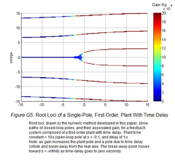
108 96 Other examples of root loci for plants with time delay. The following series of figures provide further examples of root loci for time-delay plants. Figure G3 depicts loci for a single zero, a differentiator, compensated with proportional feedback. Closedloop dynamic behavior of a proportionally-compensated double zero is illustrated with the loci in Figure G4. Figure G5 shows loci and their break-away from the real axis for a single open-loop pole, a first-order plant, with time delay. The position of the breakaway point, shown close-up in Figure G6, can be compared to the location derived through a mathematical analysis in the text, equation G37. Figure G7 shows loci for a double-pole, a second-order plant, under proportional compensation. Figure G8 shows loci for a PID-compensated first-order plant with time delay.

109 97

110 98

111 99

112 100 Break-away point for first-order plant with time delay. The point on the real axis where, as compensation gain is increased closed-loop poles collide and then depart the real axis, the break-away point, is now determined for a feedback system comprised of a first-order plant with time delay. The plant time constant is seconds so the open-loop plant pole is located at., time delay seconds, thus normalized time delay NTD 0.1. The breakaway point occurs where compensation gain k peaks in value along the real axis. Thus, must be expressed in terms of position on the real axis, then its derivative along the real axis is set to zero, 0. Compensation gain k can be expressed in terms of,, and by analyzing the characteristic equation along the real axis, (G34) or so 1 (G35) The derivative of gain along the real axis is

113 (G36) The derivative equals zero when 0, thus breakaway occurs at 1.1 (G37)

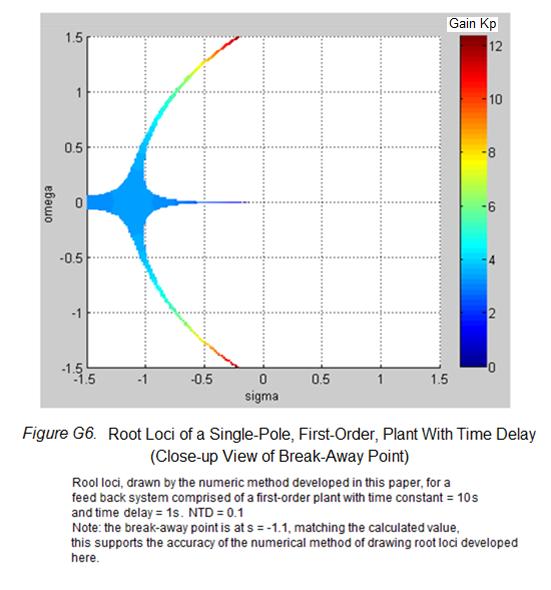
114 102

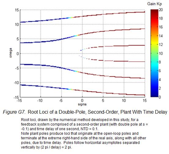
115 103

116 104

117 105 Appendix H Compensation Gain Yielding 5% Overshoot of Set Point for a First-Order Plant With Time Delay Compensation gain for a first-order plant with time delay is determined for seven values of normalized time delay. A series of seven root-locus plots, drawn by the numerical method developed in this paper, were used to identify gains as discussed in Chapter 3: Results. Gains are selected such that the dominant closed-loop poles lie at locations which correspond with a damping coefficient of 0.7 (5% overshoot), in a purely second-order system, and are tabulated and plotted below in Table H1 and Figure H1.

118 106 Table H1 Compensation Gain Yielding 5% Overshoot for a First-Order Plant With Time Delay Recommended Resulting Normalized-Time Delay, NTD Time Delay Divided by Plant Time Constant Compensation Gain (For 5% Overshoot) 2% Settling Time (Multiples of Open-Loop Settling Time) Note: Compensation gain for a first-order plant with time delay, resulting in 5% overshoot of final value, stated as a function of normalized time delay NTD. Settling times are referenced to 2% open-loop settling time, assumed to be 4 plant time constants.

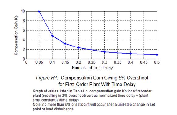
119 107