Dynamic System Response. Dynamic System Response K. Craig 1

Transcription

1 Dynamic System Response Dynamic System Response K. Craig 1

2 Dynamic System Response LTI Behavior vs. Non-LTI Behavior Solution of Linear, Constant-Coefficient, Ordinary Differential Equations Classical Operator Method Laplace Transform Method Laplace Transform Properties 1 st -Order Dynamic System Time and Frequency Response nd -Order Dynamic System Time and Frequency Response Dynamic System Response Example Problems Dynamic System Response K. Craig

3 LTI Behavior vs. Non-LTI Behavior Linear Time-Invariant (LTI) Systems A frequency-domain transfer function is limited to describing elements that are linear and time invariant severe restrictions! No real-world system meets them! Linear Time-Invariant System Properties Homogeneity: If r(t) c(t), then kr(t) kc(t) Superposition: If r 1 (t) c 1 (t) and r (t) c (t), then r 1 (t) + r (t) c 1 (t) + c (t) Time Invariance: If r(t) c(t), then r(t-t 1 ) c(t-t 1 ) Dynamic System Response K. Craig 3

4 Comments on the Principle of Superposition The principle of superposition states that if the system has an input that can be expressed as the sum of signals, then the response of the system can be expressed as the sum of the individual responses to the respective signals. Superposition applies if and only if the system is linear. Using the principle of superposition, we can solve for the system responses to a set of elementary signals. We are then able to solve for the response to a general signal simply by decomposing the given signal into a sum of the elementary components and, by superposition, concluding that the response to the general signal is sum of the responses to the elementary signals. Dynamic System Response K. Craig 4

5 In order for this process to work, the elementary signals need to be sufficiently rich that any reasonable signal can be expressed as a sum of them, and their responses have to be easy to find. The most common candidate for elementary signals for use in linear systems are the impulse and the exponential. The unit impulse δ(t) is a pulse of zero duration and infinite height. The area under the unit impulse (its strength) is equal to one. The impulse δ(t) is defined by δ(t-τ) = 0 for all t τ. It has the property that if f(t) is continuous at t = τ, then τ τ + δ(t τ )dt = 1 f( τδ ) (t τ)dτ= f(t) Dynamic System Response K. Craig 5

6 The impulse is so short and so intense that no value of f matters except over the short range where the δ occurs. The integral can be viewed as representing the function f as a sum of impulses. To find the response to an arbitrary input, the principle of superposition tells us that we need only find the response to a unit impulse. For a linear, time-invariant system, the impulse response, i.e., the response at time t to an impulse applied at time τ, can be expressed as h(t τ) because the response at time t to an input applied at time τ depends only on the difference between the time the impulse is applied and the time we are observing the response. Dynamic System Response K. Craig 6

7 For linear, time-invariant systems with input u(t), the superposition integral, called the convolution integral, is: y(t) u( )h(t )d u(t )h( )d u h = τ τ τ= τ τ τ= Here u(t) is the input to the system and h(t-τ) is the impulse response of the system. Dynamic System Response K. Craig 7

8 Assume y Convolution Example = Ae st st st Ase + kae = 0 s= k A= 1 kt y(t) = h(t) = e for t > 0 1(t) 0 t < 0 1 t 0 unit step function y + ky= u =δ (t) y(0 ) = ydt + k ydt = δ(t)dt y(0 ) y(0 ) + k(0) = 1 + y(0 ) = 1 + y + ky= 0 y(0 ) = 1 kt y(t) = h(t) = e 1(t) The response to a general input u(t) is given by the convolution of this impulse response and the input: kt y(t) e 1(t)u(t )d kt = τ τ = e u(t τ)dτ Dynamic System Response K. Craig 8 0 impulse response

9 A consequence of convolution is the concept of transfer function. y t = h( τ)u(t τ) dτ Convolution Integral () = h( τ)e dτ Input = e s(t τ) st st τ s st s h( )e e d e τ h( )e d st τ s = τ τ= τ τ = e H(s) where H(s) = h( τ)e dτ Note that both the input and output are exponential time functions and that the output differs from the input only in the amplitude H(s). The function H(s) is the transfer function from the input to output of the system. It is the ratio of the Laplace transform of the output to the Laplace transform of the input assuming all initial conditions are zero. Dynamic System Response K. Craig 9

10 If the input is the unit impulse function δ(t), then y(t) is the unit impulse response. The Laplace transform of δ(t) is 1 and the Laplace transform of y(t) is Y(s), so Y(s) = H(s). The transfer function H(s) is the Laplace transform of the unit impulse response h(t) where the Laplace transform is defined by: st H(s) = h(t)e dt st h(t)e dt since h(t) 0 for t 0 0 = = < Thus, if one wishes to characterize a linear timeinvariant system, one applies a unit impulse, and the resulting response is a description (inverse Laplace transform) of the transform function. Dynamic System Response K. Craig 10

11 A common way to use the exponential response of a linear time-invariant system is in finding the frequency response. A jωt ω j t Euler s relation is: Acos( ω t) = (e + e ) Let s = jω and, by superposition, the response to the sum of these two exponentials which make up the cosine signal, is the sum of the responses: A jωt jωt y(t) = H(j ω )e + H( j ω)e The transfer function H(jω) is a complex number that can be expressed in polar form (magnitude and phase form) as H(jω) = M(ω)e jφ(ω). A j( ω+φ t ) j( ω+φ t ) y(t) = M e + e = AM cos( ω t +φ) Dynamic System Response K. Craig 11

12 This means that if a system represented by the transfer function H(s) has a sinusoidal input with magnitude A, the output will be sinusoidal at the same frequency with magnitude AM and will be shifted in phase by the angle Φ. The response of a linear time-invariant system to a sinusoid of frequency ω is a sinusoid with the same frequency and with an amplitude ratio equal to the magnitude of the transfer function evaluated at the input frequency. The phase difference between input and output signals is given by the phase of the transfer function evaluated at the input frequency. The magnitude ratio and phase difference can be computed from the transfer function or measured experimentally. Dynamic System Response K. Craig 1

13 Transfer Functions, the basis of classical control theory, require LTI systems, but no real-world system is completely LTI. There are regions of nonlinear operation and often significant parameter variation. Examples of Linear Behavior addition, subtraction, scaling by a fixed constant, integration, differentiation, time delay, and sampling No practical control system is completely linear and most vary over time. LTI systems can be represented completely in the frequency domain. Non-LTI systems can have frequency response plots, however, these plots change depending on system operating conditions. Dynamic System Response K. Craig 13

14 Non-LTI Behavior Non-LTI behavior is any behavior that violates one or more of the three criteria for an LTI system. Within nonlinear behavior, an important distinction is whether the variation is slow or fast with respect to the loop dynamics. Slow Variation When the variation is slow, the nonlinear behavior may be viewed as a linear system with parameters that vary during operation. The dynamics can still be characterized effectively with a transfer function. However, the frequency response plots will change at different operating points. Dynamic System Response K. Craig 14

15 Fast Response If the variation of the loop parameter is fast with respect to the loop dynamics, the situation becomes more complicated. Transfer functions cannot be relied upon for analysis. The definition of fast depends on the system dynamics. Fast vs. Slow The line between fast and slow is determined by comparing the rate at which the parameter changes to the bandwidth of the control system. If the parameter variation occurs over a period of time no faster than 10 times the control loop settling time, the effect can be considered slow for most applications. Dynamic System Response K. Craig 15

16 Dealing with Nonlinear Behavior Nonlinear behavior can usually be ignored if the changes in parameter values effect the loop gain by no more than about 5%. A variation this small will be tolerated by systems with reasonable margins of stability. If a parameter varies more than that, there are at least three courses of action: Modify the plant Tune for the worst-case conditions Compensate for the nonlinearity of the control loop Dynamic System Response K. Craig 16

17 Modify the Plant Modifying the plant to reduce the parameter variation is the most straightforward solution to nonlinear behavior. It cures the problem without adding complexity to the controller or compromising system performance. This solution is commonly employed in the sense that components used in control systems are generally better (closer to LTI) than components used in open-loop systems. Enhancing the LTI behavior of a loop component can increase its cost significantly. Components for control systems are often more expensive than open-loop components. Dynamic System Response K. Craig 17

18 Tune for the Worst-Case Conditions Assuming that the variation from the non-lti behavior is slow with respect to the control loop, its effect is to change gains in the control loop. In this case, the operating conditions can be varied to produce the worst-case gains while tuning the control system. Doing so will ensure stability for all operating conditions. Tuning the system for worst-case operating conditions generally implies tuning the proportional gain of the inner loop when the plant gain is at its maximum. This ensures that the inner loop will be stable in all conditions; parameter variation will only lower the loop gain, which will reduce responsiveness but will not cause instability. Dynamic System Response K. Craig 18

19 The other loop gains (inner loop integral and the outer loops) should be stabilized when the plant gain is minimized. This is because minimizing the plant gain reduces the inner loop response; this will provide the maximum phase lag to the outer loops and again provides the worst case for stability. So tune the proportional gain with a high plant gain and tune the other gains with a low plant gain to ensure stability in all conditions. The penalty for tuning for worst case is the reduction in responsiveness. Consider the proportional gain. Because the proportional term is tuned with the highest plant gain, the loop gain will be reduced at operating points where the plant gain is low. In general, you should expect to lose responsiveness in proportion to plant variation. Dynamic System Response K. Craig 19

20 Compensate in the Control Loop Compensating for the nonlinear behavior in the controller requires that a gain equal to the inverse of the non-lti behavior be placed in the loop. This is called gain scheduling. By using gain scheduling, the impact of the non-lti behavior is eliminated from the control loop. Gain scheduling requires that the non-lti behavior be slow with respect to any transfer functions between the non-lti component and the scheduled gain. This is a less onerous requirement than being slow with respect to the loop bandwidth because the loop components are always much faster than the loop itself. Dynamic System Response K. Craig 0

21 Gain scheduling assumes that the non-lti behavior can be predicted to reasonable accuracy (generally ± 5%) based on information available to the controller. This is often the case. Many times, a dedicated control loop will be placed under the direction of a larger system controller. The more flexible system controller can be used to accumulate information on a changing gain and then modify gains inside dedicated controllers to affect the compensation. The chief shortcoming of gain scheduling via the system controller is limited speed. The system controller may be unable to keep up with the fastest plant variations. Still this solution is commonly employed because of the controller s higher level of flexibility and broader access to information. Dynamic System Response K. Craig 1

22 Solution of Linear, Constant-Coefficient Ordinary Differential Equations A basic mathematical model used in many areas of engineering is the linear, ordinary differential equation with constant coefficients: n n 1 dqo d qo dqo an + a n n a n a0qo = dt dt dt d q d q dq b b b b q dt dt dt m m 1 i i i m + m m m i q o is the output (response) variable of the system q i is the input (excitation) variable of the system a n and b m are the physical parameters of the system Dynamic System Response K. Craig

23 Straightforward analytical solutions are available no matter how high the order n of the equation. Review of the classical operator method for solving linear differential equations with constant coefficients will be useful. When the input q i (t) is specified, the right hand side of the equation becomes a known function of time, f(t). The classical operator method of solution is a three-step procedure: Find the complimentary (homogeneous) solution q oc for the equation with f(t) = 0. Find the particular solution q op with f(t) present. Get the complete solution q o = q oc + q op and evaluate the constants of integration by applying known initial conditions. Dynamic System Response K. Craig 3

24 Step 1 To find q oc, rewrite the differential equation using the differential operator notation D = d/dt, treat the equation as if it were algebraic, and write the system characteristic equation as: ad + a D + + ad+ a = 0 n n 1 n n Treat this equation as an algebraic equation in the unknown D and solve for the n roots (eigenvalues) s 1, s,..., s n. Since root finding is a rapid computerized operation, we assume all the roots are available and now we state rules that allow one to immediately write down q oc. Dynamic System Response K. Craig 4

25 Real, unrepeated root s 1 : oc 1 Real root s repeated m times: m q = c e + c te + c t e + + c t e When the a 0 to a n in the differential equation are real numbers, then any complex roots that might appear always come in pairs a ± ib: at qoc = ce sin(bt +φ) For repeated root pairs a ± ib, a ± ib, and so forth, we have: The c s and φ s are constants of integration whose numerical values cannot be found until the last step. Dynamic System Response K. Craig 5 q = c e st st st st oc 0 1 m q = c e sin(bt +φ ) + c te sin(bt +φ ) + at at oc st 1

26 Step The particular solution q op takes into account the "forcing function" f(t) and methods for getting the particular solution depend on the form of f(t). The method of undetermined coefficients provides a simple method of getting particular solutions for most f(t)'s of practical interest. To check whether this approach will work, differentiate f(t) over and over. If repeated differentiation ultimately leads to zeros, or else to repetition of a finite number of different time functions, then the method will work. Dynamic System Response K. Craig 6

27 The particular solution will then be a sum of terms made up of each different type of function found in f(t) and all its derivatives, each term multiplied by an unknown constant (undetermined coefficient). If f(t) or one of its derivatives contains a term identical to a term in q oc, the corresponding terms should be multiplied by t. This particular solution is then substituted into the differential equation making it an identity. Gather like terms on each side, equate their coefficients, and obtain a set of simultaneous algebraic equations that can be solved for all the undetermined coefficients. Dynamic System Response K. Craig 7

28 Step 3 We now have q oc (with n unknown constants) and q op (with no unknown constants). The complete solution q o = q oc + q op. The initial conditions are then applied to find the n unknown constants. Dynamic System Response K. Craig 8

29 Certain advanced analysis methods are most easily developed through the use of the Laplace Transform. A transformation is a technique in which a function is transformed from dependence on one variable to dependence on another variable. Here we will transform relationships specified in the time domain into a new domain wherein the axioms of algebra can be applied rather than the axioms of differential or difference equations. The transformations used are the Laplace transformation (differential equations) and the Z transformation (difference equations). The Laplace transformation results in functions of the time variable t being transformed into functions of the frequency-related variable s. Dynamic System Response K. Craig 9

30 The Z transformation is a direct outgrowth of the Laplace transformation and the use of a modulated train of impulses to represent a sampled function mathematically. The Z transformation allows us to apply the frequency-domain analysis and design techniques of continuous control theory to discrete control systems. One use of the Laplace Transform is as an alternative method for solving linear differential equations with constant coefficients. Although this method will not solve any equations that cannot be solved also by the classical operator method, it presents certain advantages. Dynamic System Response K. Craig 30

31 Separate steps to find the complementary solution, particular solution, and constants of integration are not used. The complete solution, including initial conditions, is obtained at once. There is never any question about which initial conditions are needed. In the classical operator method, the initial conditions are evaluated at t = 0 +, a time just after the input is applied. For some kinds of systems and inputs, these initial conditions are not the same as those before the input is applied, so extra work is required to find them. The Laplace Transform method uses the conditions before the input is applied; these are generally physically known and are often zero, simplifying the work. Dynamic System Response K. Craig 31

32 For inputs that cannot be described by a single formula for their entire course, but must be defined over segments of time, the classical operator method requires a piecewise solution with tedious matching of final conditions of one piece with initial conditions of the next. The Laplace Transform method handles such discontinuous inputs very neatly. The Laplace Transform method allows the use of graphical techniques for predicting system performance without actually solving system differential equations. All theorems and techniques of the Laplace Transform derive from the fundamental definition for the direct Laplace Transform F(s) of the time function f(t): [ ] st L f (t) F(s) f (t)e dt t > 0 s complex variable i 0 = = = =σ+ ω Dynamic System Response K. Craig 3

33 This integral cannot be evaluated for all f(t)'s, but when it can, it establishes a unique pair of functions, f(t) in the time domain and its companion F(s) in the s domain. Comprehensive tables of Laplace Transform pairs are available. Signals we can physically generate always have corresponding Laplace transforms. When we use the Laplace Transform to solve differential equations, we must transform entire equations, not just isolated f(t) functions, so several theorems are necessary for this. Linearity (Superposition and Amplitude Scaling) Theorem: [ ] [ ] [ ] L a f (t) + a f (t) = L a f (t) + L a f (t) = a F (s) + a F (s) Dynamic System Response K. Craig 33

34 Differentiation Theorem: df L = sf(s) f(0) dt df df L s F(s) sf(0) (0) dt = dt n n 1 df n n 1 n df d f L s F(s) s f (0) s (0) (0) n n 1 dt = dt dt f(0), (df/dt)(0), etc., are initial values of f(t) and its derivatives evaluated numerically at a time instant before the driving input is applied. Multiplication by Time: Multiplication by time corresponds to differentiation in the frequency domain. d Ltf(t) [ ] = F(s) ds Dynamic System Response K. Craig 34

35 Integration Theorem: ( n) Again, the initial values of f(t) and its integrals are evaluated numerically at a time instant before the driving input is applied. Convolution Theorem: ( 1) F(s) f (0) L f(t)dt = + s s L f (t) = + Convolution in the time domain corresponds to multiplication in the frequency domain. L f (t) f (t) = F (s)f (s) Dynamic System Response K. Craig 35 ( k) n F(s) f (0) n n k+ 1 s k= 1 s ( n) n (-0) where f (t) = f(t)(dt) and f (t) = f(t) [ ] 1 1

36 Time Delay Theorem: The Laplace Transform provides a theorem useful for the dynamic system element called dead time (transport lag) and for dealing efficiently with discontinuous inputs. u(t) = 1.0 t > 0 u(t) = 0 t < 0 u(t a) = 1.0 t > a u(t a) = 0 t < a [ ] as Lf(t a)u(t a) = e F(s) Time Scaling Theorem: If the time t is scaled by a factor a, then the Laplace transform of the time-scaled signal is 1 s F a a Dynamic System Response K. Craig 36

37 Final Value Theorem: If we know Q 0 (s), q 0 ( ) can be found quickly without doing the complete inverse transform by use of the final value theorem. lim f (t) = lim sf(s) t s 0 This is true if the system and input are such that the output approaches a constant value as t approaches. The DC gain of a system, the steady-state value of the unit-step response, is given by: 1 DC Gain = lims G(s) = lim G(s) s 0 Initial Value Theorem: s s 0 This theorem is helpful for finding the value of f(t) just after the input has been applied, i.e., at t = 0 +. In getting the F(s) needed to apply this theorem, our usual definition of initial conditions as those before the input is applied must be used. lim f (t) = lim sf(s) t 0 s Dynamic System Response K. Craig 37

38 Impulse Function δ(t) p(t) 1/b Approximating function for the unit impulse function b t δ (t) = lim p(t) δ (t) = 0 t 0 b 0 +ε ε δ (t)dt = 1 ε> 0 du 1 L [ (t)] L δ = = su(s) = s = 1.0 dt s The step function is the integral of the impulse function, or conversely, the impulse function is the derivative of the step function. Dynamic System Response K. Craig 38

39 When we multiply the impulse function by some number, we increase the strength of the impulse, but strength now means area, not height as it does for ordinary functions. An impulse that has an infinite magnitude and zero duration is mathematical fiction and does not occur in physical systems. If, however, the magnitude of a pulse input to a system is very large and its duration is very short compared to the system time constants, then we can approximate the pulse input by an impulse function. The impulse input supplies energy to the system in an infinitesimal time. Dynamic System Response K. Craig 39

40 Approximate and Exact Impulse Functions If e s =1.0 (unit step function), its derivative is the unit impulse function with a strength (or area) of one unit. This non-rigorous approach does produce the correct result. Dynamic System Response K. Craig 40

41 Inverse Laplace Transformation A convenient method for obtaining the inverse Laplace transform is to use a table of Laplace transforms. In this case, the Laplace transform must be in a form immediately recognizable in such a table. If a particular transform F(s) cannot be found in a table, then we may expand it into partial fractions and write F(s) in terms of simple functions of s for which inverse Laplace transforms are already known. These methods for finding inverse Laplace transforms are based on the fact that the unique correspondence of a time function and its inverse Laplace transform holds for any continuous time function. Dynamic System Response K. Craig 41

42 Dynamic System Response K. Craig 4

43 Time Response & Frequency Response 1 st -Order Dynamic System Example: RC Low-Pass Filter in out in out Dynamic System Investigation of the RC Low-Pass Filter Dynamic System Response K. Craig 43

44 Zero-Order Dynamic System Model Step Response Frequency Response Dynamic System Response K. Craig 44

45 Validation of a Zero-Order Dynamic System Model Dynamic System Response K. Craig 45

46 1 st -Order Dynamic System Model τ = time constant K = steady-state gain t = τ Slope at t = 0 q Kq = τ t is e τ Kq q = = τ Dynamic System Response o o t 0 K. Craig 46 is

47 How would you determine if an experimentallydetermined step response of a system could be represented by a first-order system step response? q(t) o = Kqis 1 e q(t) Kq o Kq is q(t) = Kq is t o 1 e τ is = e t τ t τ q(t) o t t log10 1 = log10 e = Kqis τ τ Straight-Line Plot: q(t) o log10 1 vs. t Kqis Slope = /τ Dynamic System Response K. Craig 47

48 This approach gives a more accurate value of τ since the best line through all the data points is used rather than just two points, as in the 63.% method. Furthermore, if the data points fall nearly on a straight line, we are assured that the instrument is behaving as a first-order type. If the data deviate considerably from a straight line, we know the system is not truly first order and a τ value obtained by the 63.% method would be quite misleading. An even stronger verification (or refutation) of first-order dynamic characteristics is available from frequencyresponse testing. If the system is truly first-order, the amplitude ratio follows the typical low- and highfrequency asymptotes (slope 0 and 0 db/decade) and the phase angle approaches -90 asymptotically. Dynamic System Response K. Craig 48

49 If these characteristics are present, the numerical value of τ is found by determining ω (rad/sec) at the breakpoint and using τ = 1/ω break. Deviations from the above amplitude and/or phase characteristics indicate non-first-order behavior. Dynamic System Response K. Craig 49

50 What is the relationship between the unit-step response and the unit-ramp response and between the unit-impulse response and the unit-step response? For a linear time-invariant system, the response to the derivative of an input signal can be obtained by differentiating the response of the system to the original signal. For a linear time-invariant system, the response to the integral of an input signal can be obtained by integrating the response of the system to the original signal and by determining the integration constants from the zero-output initial condition. Dynamic System Response K. Craig 50

51 Unit-Step Input is the derivative of the Unit-Ramp Input. Unit-Impulse Input is the derivative of the Unit-Step Input. Once you know the unit-step response, take the derivative to get the unit-impulse response and integrate to get the unit-ramp response. Dynamic System Response K. Craig 51

52 System Frequency Response Dynamic System Response K. Craig 5

53 Bode Plotting of 1 st -Order Frequency Response 0.01 = 40 db 0.1 = 0 db 0.5 = 6 db 1.0 = 0 db.0 = 6 db 10.0 = 0 db = 40 db db = 0 log 10 (amplitude ratio) decade = 10 to 1 frequency change octave = to 1 frequency change Dynamic System Response K. Craig 53

54 Analog Electronics: RC Low-Pass Filter Time Response & Frequency Response e RCs + 1 R e in out i = in Cs 1 i out eout 1 1 = = when iout = 0 e RCs + 1 τ s + 1 in Dynamic System Response K. Craig 54

55 Time Response to Unit Step Input Amplitude R = 15 KΩ C = 0.01 μf Time (sec) x 10-4 Time Constant τ = RC Dynamic System Response K. Craig 55

56 Time Constant τ Time it takes the step response to reach 63% of the steady-state value Rise Time T r =. τ Time it takes the step response to go from 10% to 90% of the steady-state value Delay Time T d = 0.69 τ Time it takes the step response to reach 50% of the steady-state value Dynamic System Response K. Craig 56

57 Frequency Response R = 15 KΩ C = 0.01 μf Bandwidth = 1/τ e K K 0 K out 1 (i ω ) = = = tan ωτ e 1 in iωτ + 1 ( ωτ ) + 1 tan ωτ ( ωτ ) + 1 Dynamic System Response K. Craig 57

58 Bandwidth The bandwidth is the frequency where the amplitude ratio drops by a factor of = -3dB of its gain at zero or low-frequency. For a 1 st -order system, the bandwidth is equal to 1/τ. The larger (smaller) the bandwidth, the faster (slower) the step response. Bandwidth is a direct measure of system susceptibility to noise, as well as an indicator of the system speed of response. Dynamic System Response K. Craig 58

59 Amplitude Ratio = = -3 db Phase Angle = -45 Input Response to Input 1061 Hz Sine Wave amplitude Output time (sec) x 10-3 Dynamic System Response K. Craig 59

60 Time Response & Frequency Response nd -Order Dynamic System Example: -Pole, Low-Pass, Active Filter R 4 R 7 C 5 e in R 1 C R R e out Dynamic System Investigation of the Two-Pole, Low-Pass, Active Filter Dynamic System Response K. Craig 60

61 Physical Model Ideal Transfer Function R 7 1 R eout 6 R1R3CC 5 (s) = ein s s+ RC RC RC RRCC Dynamic System Response K. Craig 61

62 nd -Order Dynamic System Model dq0 dq = 0 i a a a q b q dt dt q0 = Kqi ω dq0 ζ dq0 n dt ωn dt a 0 ω n = a 1 ζ = 0 0 K = steady-state gain 0 a a a b a undamped natural frequency damping ratio Step Response of a nd -Order System Dynamic System Response K. Craig 6

63 1 dq0 ς dq Step Response 0 + ζ + q 0 = Kqi of a ωn dt ωn dt nd -Order System Underdamped 1 ( ) ζωn q t 1 o = Kqis 1 e sin ω n 1 ζ t + sin 1 ζ ζ< 1 1 ζ Critically Damped ωn ( ) t qo = Kq is 1 1+ωnt e ζ = 1 Overdamped ( ζ+ ζ ) ζ+ ζ 1 1 ωnt 1 e ζ 1 qo = Kq is ζ > 1 ζ ζ 1 ( ζ ζ 1) ωnt + e ζ 1 Dynamic System Response K. Craig 63

64 Frequency Response of a nd -Order System Laplace Transfer Function Q Q o i ( s) = s ω n K ζs ω n Sinusoidal Transfer Function Qo K 1 ζ ( iω ) = tan Q i ω ω n ω 4ζ ω 1 + ωn ω ωn ω n Dynamic System Response K. Craig 64

65 Frequency Response of a nd -Order System Dynamic System Response K. Craig 65

66 -40 db per decade slope Frequency Response of a nd -Order System Dynamic System Response K. Craig 66

67 Some Observations When a physical system exhibits a natural oscillatory behavior, a 1 st -order model (or even a cascade of several 1 st -order models) cannot provide the desired response. The simplest model that does possess that possibility is the nd -order dynamic system model. This system is very important in control design. System specifications are often given assuming that the system is nd order. For higher-order systems, we can often use dominant pole techniques to approximate the system with a nd -order transfer function. Dynamic System Response K. Craig 67

68 Damping ratio ζ clearly controls oscillation; ζ < 1 is required for oscillatory behavior. The undamped case (ζ = 0) is not physically realizable (total absence of energy loss effects) but gives us, mathematically, a sustained oscillation at frequency ω n. Natural oscillations of damped systems are at the damped natural frequency ω d, and not at ω n. ω d =ωn 1 ζ In hardware design, an optimum value of ζ = 0.64 is often used to give maximum response speed without excessive oscillation. Undamped natural frequency ω n is the major factor in response speed. For a given ζ response speed is directly proportional to ω n. Dynamic System Response K. Craig 68

69 Thus, when nd -order components are used in feedback system design, large values of ω n (small lags) are desirable since they allow the use of larger loop gain before stability limits are encountered. For frequency response, a resonant peak occurs for ζ < The peak frequency is ω p and the peak amplitude ratio depends only on ζ. ω p =ωn 1 ζ peak amplitude ratio = ζ 1 ζ Bandwidth The bandwidth is the frequency where the amplitude ratio drops by a factor of = -3dB of its gain at zero or low-frequency. Dynamic System Response K. Craig 69 K

70 For a 1 st -order system, the bandwidth is equal to 1/τ. The larger (smaller) the bandwidth, the faster (slower) the step response. Bandwidth is a direct measure of system susceptibility to noise, as well as an indicator of the system speed of response. For a nd -order system: BW = ω 1 ζ + 4ζ + 4ζ 4 As ζ varies from 0 to 1, BW varies from 1.55ω n to 0.64ω n. For a value of ζ = 0.707, BW = ω n. For most design considerations, we assume that the bandwidth of a nd -order all pole system can be approximated by ω n. Dynamic System Response K. Craig 70 n

71 G(s) = Kω s s n + ςω n +ωn s = ςω ± iω 1 ς s 1, n n = σ± iω 1, d Location of Poles of Transfer Function σt σ y() t = 1 e cosω dt+ sinωdt ωd 1.8 t r rise time ω n 4.6 t settling time ςω s n πς 1 ς Mp = e ( 0 ζ < 1 ) overshoot ζ 1 0 ζ ( ) All-Pole nd -Order Step Response Dynamic System Response K. Craig 71

72 ω n 1.8 t r σ 4.6 t s ( p ) ζ M 0 ζ 0.6 Time-Response Specifications vs. Pole-Location Specifications Dynamic System Response K. Craig 7

73 Dynamic System Response K. Craig 73

74 Experimental Determination of ζ and ω n ζ and ω n can be obtained in a number of ways from step or frequency-response tests. For an underdamped second-order system, the values of ζ and ω n may be found from the relations: π T = ω d πζ 1 ζ 1 p e M = ζ = π + 1 log ( ) e M p ωd π ω d =ωn 1 ζ ω n = = 1 ζ T 1 ζ Dynamic System Response K. Craig 74

75 Logarithmic Decrement δ is the natural logarithm of the ratio of two successive amplitudes. ( ) x() t ( + T) ζωnt δ= ln = ln ( e ) =ζωnt x t ζω π ζω π πζ ζ= n n = = = ω d ωn 1 ζ 1 ζ δ= 1 ln n B δ B π +δ 1 n+ 1 Free Response of a nd -Order System π T = ω d ζωnt () = ( ω +φ) x t Be sin t d Dynamic System Response K. Craig 75

76 If several cycles of oscillation appear in the record, it is more accurate to determine the period T as the average of as many distinct cycles as are available rather than from a single cycle. If a system is strictly linear and second-order, the value of n is immaterial; the same value of ζ will be found for any number of cycles. Thus if ζ is calculated for, say, n = 1,, 4, and 6 and different numerical values of ζ are obtained, we know that the system is not following the postulated mathematical model. For overdamped systems (ζ > 1.0), no oscillations exist, and the determination of ζ and ω n becomes more difficult. Usually it is easier to express the system response in terms of two time constants. Dynamic System Response K. Craig 76

77 For the overdamped step response: q Kq t o τ 1 τ ( ζ+ ζ ) ζ+ ζ 1 1 ωnt 1 e ζ 1 qo = Kq is ζ > 1 ζ ζ 1 ( ζ ζ 1) ωnt + e ζ 1 τ1 τ e e 1 = + τ τ τ τ is 1 1 t where τ 1 1 τ ζ ζ ω ζ + ζ ω ( ) ( ) 1 1 n 1 n Dynamic System Response K. Craig 77

78 To find τ 1 and τ from a step-function response curve, we may proceed as follows: Define the percent incomplete response R pi as: q o R pi Kqis Plot R pi on a logarithmic scale versus time t on a linear scale. This curve will approach a straight line for large t if the system is second-order. Extend this line back to t = 0, and note the value P 1 where this line intersects the R pi scale. Now, τ 1 is the time at which the straight-line asymptote has the value 0.368P 1. Dynamic System Response K. Craig 78

79 Now plot on the same graph a new curve which is the difference between the straight-line asymptote and R pi. If this new curve is not a straight line, the system is not second-order. If it is a straight line, the time at which this line has the value 0.368(P 1-100) is numerically equal to τ. Frequency-response methods may also be used to find τ 1 and τ. Dynamic System Response K. Craig 79

80 Step-Response Test for Overdamped Second-Order Systems Dynamic System Response K. Craig 80

81 Frequency-Response Test of Second-Order Systems Dynamic System Response K. Craig 81

82 Dynamic System Response Examples Dynamic System Response K. Craig 8

83 Problem Statement An underdamped nd -order system model has the following transfer function: Kωn G(s) = s + ςω s+ ω Part 1: s = ςω ± iω 1 ς 1, n n 1, d Using the properties and formulas for nd -order systems, discuss the relationships between the step-response-parameters rise time, settling time, and overshoot, and the frequency-responseparameters bandwidth and peak amplitude as the model parameters vary. Use plots as needed in your presentation. Dynamic System Response K. Craig 83 s = σ± iω n n

84 Suggestion: Pick a base system. Generate 4 families of plots ω d constant, vary σ σ constant, vary ω d ω n constant, vary ζ ζ constant, vary ω n Show both time-response and frequencyresponse plots. Include discussion. Dynamic System Response K. Craig 84

85 Part : Investigate the effects on the time (step) response and frequency response of adding a real pole or a real zero to the nd -order transfer function. The pole and zero are added separately. In classical deign using root-locus or frequency-response techniques, real poles and zeros are added (lead, lag, lead-lag controllers) to modify system dynamics, and so it is important to have a good understanding of these effects. Use plots as needed in your presentation. Dynamic System Response K. Craig 85

86 Suggestion: Pick a base second-order system. Add a negative real pole (s + p) to the transfer function and move the pole from the left towards the origin and describe its effect on the time-response and frequencyresponse plots. Add a negative real zero (s + z) to the transfer function and move the zero from the left towards the origin and describe its effect on the time-response and frequencyresponse plots. Dynamic System Response K. Craig 86

87 Part 3: Now add a positive real zero to your base second-order system and evaluate the step response for the system. Explain your observations. Physically, what might cause a transfer function to have a right-half plane zero? Dynamic System Response K. Craig 87

88 Problem Solution ωn ω d +σ G(s) = = s + ζω ns+ω n s + σ s + ( ω d +σ ) Base System σ = 1 ω n = G(s) = s + s+ ω d = 1 ζ= Effects of σ: ω d = 1, σ = [0.5, 1, 5] Effects of ω d : σ = 1, ω d = [0.5, 1, 5] Effects of ω n : ζ = 0.707, ω n = [0.5,, 5 ] Effects of ζ: ω n =, ζ = [0.866, 0.707, 0.5] Dynamic System Response K. Craig 88

89 Effects of varying σ ω d = 1, σ = [0.5, 1, 5] σ = 0.5 σ = 5 σ = 5 As σ increases: t s decreases t r decreases M p decreases BW increases σ = 0.5 σ = 0.5 σ = 5 Dynamic System Response K. Craig 89

90 Effects of varying ω d σ = 1, ω d = [0.5, 1, 5] ω d = 5 ω d = 0.5 ω d = 5 As ω d increases: t s is fixed t r decreases M p increases BW increases ω d = 0.5 ω d = 0.5 ω d = 5 Dynamic System Response K. Craig 90

91 Effects of varying ω n ζ = 0.707, ω n = [0.5,, 5 ] ω n = 0.5 ω n = 5 ω n = 5 As ω n increases: t s decreases t r decreases M p is fixed BW increases ω n = 0.5 ω n = 0.5 ω n = 5 Dynamic System Response K. Craig 91

92 ζ =0.5 Effects of varying ζ ω n =, ζ = [0.866, 0.707, 0.5] ζ =0.866 ζ = 0.5 As ζ increases: t s increases t r decreases M p increases BW increases ζ =0.866 ζ =0.866 ζ =0.5 Dynamic System Response K. Craig 9

93 Effect of an Additional LHP Pole ωn ω d +σ G(s) = = s + ζω ns+ω n s + σ s + ( ω d +σ ) Base System G( s) = σ = 1 ω n = s + s+ ω d = 1 ζ= Additional Pole G(s) = = ( ) ps 1 (s s ) 1 3 ps + (p+ 1)s + (p+ )s+ p = [0, 0., 1, ] Dynamic System Response K. Craig 93

94 Effect of an Additional Pole p = [0, 0., 1, ] increasing p As p increases (pole gets closer to the origin): t s increases t r increases M p decreases to zero BW decreases increasing p increasing p Dynamic System Response K. Craig 94

95 Effect of a LHP Zero G(s) Base System Add a Zero ( ) = G s ω ω +σ = = s s s s ( ) n d + ζω n +ω n + σ + ω d +σ σ = 1 s + s+ ω d = 1 ω = n ζ= G(s) = (zs + 1) + + (s s ) z = [0, 0., 1, ] Dynamic System Response K. Craig 95

96 Effect of a LHP Zero z = [0,0., 1, ] increasing z As z increases (zero gets closer to the origin): t s increases t r decreases M p increases BW increases increasing z increasing z Dynamic System Response K. Craig 96

97 Effect of a RHP Zero ωn ω d +σ G(s) = = s + ζω ns+ω n s + σ s + ( ω d +σ ) Base System G(s) = ( ) = G s Add a RHP Zero + + (s s ) s + s+ ( s + ) σ = 1 ω = 1 s G(s) 1 = + = (s + s + ) (s + s + ) (s + s + ) s ( s+ ) G(s) = = (s + s + ) (s + s + ) (s + s + ) Dynamic System Response K. Craig 97 d ω = n ζ= G(s) plus its derivative G(s) minus its derivative

98 G 1 (s) G(s) G (s) Dynamic System Response K. Craig 98

99 s s s + + s s s + + s s Dynamic System Response K. Craig 99

100 s + s+ s s s s + + s s Dynamic System Response K. Craig 100

101 Problem Statement Satellites often require attitude control for proper orientation of antennas and sensors with respect to the earth. This is a three-axis, attitude-control system. To gain insight into the three-axis problem we often consider one axis at a time. For the one-axis problem, the plant transfer function is G(s) = 1/s. This results from the equation of motion: Jθ = T J is the moment of inertia of the satellite about its mass center, T is the control torque applied by the thrusters, and θ is the angle of the satellite axis with respect to an inertial reference frame, which must have no angular acceleration. Dynamic System Response K. Craig 101

102 A controller has been designed (see below). What are the time-response and frequency-response performance indicators for this closed-loop system. s+ 3 G c(s) = 0 s + 1 Assuming the controller is to be implemented digitally, approximate the time lag from the D/A converter to be: /T s+ /T Dynamic System Response K. Craig 10

103 Determine the closed-loop system root locations for sample rates ω s = 5 Hz, 10 Hz, and 0 Hz, where the sample period T = 1/ω s seconds. Plot the unit step responses for the analog system and for each sample rate and compare. State your observations regarding closed-loop stability. How fast do you think one should sample in order to have a reasonably smooth response? The closed-loop block diagram is shown below: R(s) /T 1 Σ Controller + s+ /T s - C(s) Dynamic System Response K. Craig 103

104 Problem Solution Open-Loop Transfer Function Closed-Loop Transfer Function s s 1 s + s s+ 1 s 0(s + 3) = s + 1 s s (s 1s 0s 660) Closed-Loop Poles: -4.55, -8.3 ± 8.80i Closed-Loop Zero: -3 Dynamic System Response K. Craig 104

105 Closed-Loop Step Response M p = 9.4% % t s = sec t r = sec Dynamic System Response K. Craig 105

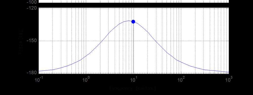
106 Open-Loop Frequency-Response Plot GM = PM = 47.9º Dynamic System Response K. Craig 106

107 Closed-Loop Frequency-Response Plot -3dB BW = 16.5 rad/sec Dynamic System Response K. Craig 107

108 Time Delay τ = T/ Approximation 1 τ s+ 1 T = 0., 0.1, 0.05 τ = 0.1, 0.05, 0.05 R(s) /T 1 Σ Controller + s+ /T s - = G c(s) 0 s + 1 C(s) s+ 3 C 0(s + 3) (s) = τ + τ R s (1 1)s 1s 0s 660 Closed-Loop Poles: τ = 0.1: -5.78, ± 8.31i, τ = 0.05: -31.7, -.65 ± 9.87i, τ = 0.05: -46.8, ± 10.44i, -4.1 Dynamic System Response K. Craig 108

109 Step Response τ = 0.1 τ = 0.05 τ = 0.05 τ = 0 Dynamic System Response K. Craig 109