Math Week 1 notes
|
|
|
- Sherilyn Burke
- 5 years ago
- Views:
Transcription
1 Math Week 1 notes We will not necessarily finish the material from a given day's notes on that day. We may also add or subtract some material as the week progresses, but these notes represent an in-depth outline of what we will cover. These notes are for sections , and part of 1.4. Monday January 12 Go over course information on syllabus and course homepage: Notice that there is homework due this Friday, and our first quiz. Then, let's begin! Section 1.1 Introduction to differential equations What is an n th order differential equation (DE)? any equation involving a function y = y x and its derivatives, for which the highest derivative appearing in the equation is the n th one, y n x ; i.e. any equation which can be written as F x, y x, y x, y x,...y n x = 0. Exercise 1: Which of the following are differential equations? For each DE determine the order. 2 a) For y = y x, y x sin y x = 0 b) For x = x t, x t = 3 x t 10 x t. c) For x = x t, x = 3 x 10 x. d) For z = z r, z r 4 z r. e) For y = y x, y = y 2.
2 Definitions: A function y x solves the differential equation F x, y, y, y, y n = 0 on some interval I (or is a solution function for the differential equation) means that y x makes the differential equation a true equality for all x in I. A 1 st order DE is an equation involving a function and its first derivative. We may chose to write the function and variable as y = y x. In this case the differential equation is an equation equivalent to one of the form F x, y, y = 0. Chapters 1-2 are about first order differential equations. For first order differential equations as above we can often use algebra to solve for y in order to get what we call the standard form for the first order DE: y = f x, y. If we want our solution function to a first order DE to also satisfy y x 0 = y 0, and if our DE is written in standard form, then we say that we are stuing an initial value problem (IVP): y = f x, y y x 0 = y 0. If we can find a solution function y x that makes both equations of the the initial value problem true, then we say that y x solves the initial value problem. Exercise 2: Consider the differential equation dx = y2 from (1e). a) Show that functions y x = 1 C b) Find the appropriate value of C to solve the initial value problem y = y 2 x solve the DE (on any interval not containing the constant C). y 1 = 2.

3 2c) What is the largest interval on which your solution to 2b is defined as a differentiable function? Why? 2d) Do you expect that there are any other solutions to the IVP in 2b? Hint: The graph of the IVP solution function we found is superimposed onto a "slope field" below, where the line segment slopes at points x, y have values y 2 (because solution graphs to our differential equation will have those slopes, according to the differential equation). This might give you some intuition about whether you expect more than one solution to the IVP.
4 important course goals: understand some of the key differential equations which arise in modeling real-world namical systems from science, mathematics, engineering; how to find the solutions to these differential equations if possible; how to understand properties of the solution functions (sometimes even without formulas for the solutions) in order to effectively model or to test models for namical systems. In fact, you've encountered differential equations in previous mathematics and/or physics classes. For example: 1 st order differential equations: rate of change of function depends in some way on the function value, the variable value, and nothing else. For example, you've studied the population growth/decay differential equation for P = P t, and k a constant, given by P t = k P t and having applications in biology, physics, finance. In this model, how fast the "population" changes is proportional to the population. 2 nd order DE's: Newton's second law (change in momentum equals net forces) often leads to second order differential equations for particle position functions x = x t in physics. Exercise 3: The mathematical model in which the time rate of change of a population P t is proportional to that population is expressed mathematically as dp dt = k P where k is the proportionality constant. 3a) Find all solutions to this differential equation by using the chain rule backwards. 3b) The method of "separation of variables" is taught in most Calc I courses, and we'll cover it in detail in section 1.4. It's an algorithm which hides the "chain rule backwards" technique by treating the derivative dp dt as a quotient of differentials. Recall this magic algorithm to recover the solutions from 3a.
5 Exercise 4) Newton's law of cooling is a model for how objects are heated or cooled by the temperature of an ambient medium surrounding them. In this model, the bo temperature T = T t changes at a rate proportional to to the difference between it and the ambient temperature A t. In the simplest models A is constant. a) Use this model to derive the differential equation dt = k T A. dt b) Would the model have been correct if we wrote dt = k T A instead? dt c) Use this model to partially solve a murder mystery: At 3:00 p.m. a deceased bo is found. Its temperature is 70 F. An hour later the bo temperature has decreased to 60. It's been a winter inversion in SLC, with constant ambient temperature 30. Assuming the Newton's law model, estimate the time of death.
6 Math Wed January 11 HW due Friday... Quiz Friday... Review from Monday. What were the main ideas we talked about? At the end of today's notes is the justification for "separation of variables". We will go over that at some point today. Section 1.2: differential equations equivalent to ones of the form y x = f x which we solve by direct antidifferentiation y x = f x dx = F x C. Exercise 1 Solve the initial value problem dx = x x2 4 y 0 = 0
7 An important class of such problems arises in physics, usually as velocity/acceleration problems via Newton's second law. Recall that if a particle is moving along a number line and if x t is the particle position function at time t, then the rate of change of x t (with respect to t) namely x t, is the velocity function. If we write x t = v t then the rate of change of velocity v t, namely v t, is called the acceleration function a t, i.e. x t = v t = a t. Thus if a t is known, e.g. from Newton's second law that force equals mass times acceleration, then one can antidifferentiate once to find velocity, and one more time to find position. Exercise 2: a) If the units for position are meters m and the units for time are seconds s, what are the units for velocity and acceleration? (These are mks units.) b) Same question, if we use the English system in which length is measured in feet and time in seconds. Could you convert between mks units and English units? Exercise 3: A projectile with very low air resistance is fired almost straight up from the roof of a building 30 meters high, with initial velocity 50 m/s. Its initial horizontal velocity is near zero, but large enough so that the object lands on the ground rather than the roof. a) Neglecting friction, how high will the object get above ground? b) When does the object land?
8 Here's another fun example from section 1.2, which also reviews important ideas from Calculus - in particular we will see how the fact that the slope of a graph y = g x is the derivative can lead to first dx order differential equations. Exercise 4: (See "A swimmer's Problem" and Example 4 in section 1.2). A swimmer wishes to cross a river of width w = 2 a, by swimming directly towards the opposite side, with constant transverse velocity v S. The river velocity is fastest in the middle and is given by an even function of x, for a x a. The velocity equal to zero at the river banks. For example, it could be that v R x = v 0 1 a 2. See the configuration sketches below. a) Writing the swimmer location at time t as x t, y t, translate the information above into expressions for x t and y t. b) The parametric curve describing the swimmer's location can also be expressed as the graph of a function y = y x. Show that y x satisfies the differential equation dx = v 0 1 v S a 2. c) Compute an integral or solve a DE, to figure out how far downstream the swimmer will be when she reaches the far side of the river. x 2 x 2
9 Exercise 5: Suppose the acceleration function is a negative constant a, x t = a. (This could happen for vertical motion, e.g. near the earth's surface with a = g 9.8 m s 2 32 ft well as in other situations.) a) Write x 0 = x 0, v 0 = v 0 for the initial position and velocity. Find formulas for v t and x t. b) Assuming x 0 = 0 and v 0 0, show that the maximum value of x t is x max = 1 2 a. (This formula may help with some homework problems.) v 0 2 s 2, as
10 1.4 Separable DE's: Important applications, as well as a lot of the examples we stu in slope field discussions of section 1.3 are separable DE's. So let's discuss precisely what they are, and why the separation of variables algorithm works. Definition: A separable first order DE for a function y = y x is one that can be written in the form: dx = f x y. It's more convenient to rewrite this DE as 1 = f x, y dx (as long as y 0). Writing g y = 1 the differential equation reads y g y dx = f x. Solution (math justified): The left side of the modified differential equation is short for g y x if G y is any antiderivative of g y, then we can rewrite this as G y x y x which by the chain rule (read backwards) is nothing more than d dx G y x. And the solutions to d dx G y x = f x are G y x = f x dx = F x C. dx. And where F x is any antiderivative of f x. Thus solutions y x to the original differential equation satisify G y = F x C. This expresses solutions y x implicitly as functions of x. You may be able to use algebra to solve this equation explicitly for y = y x, and (working the computation backwards) y x will be a solution to the DE. (Even if you can't algebraically solve for y x, this still yields implicitly defined solutions.) Solution (differential magic): Treat as a quotient of differentials, dx, and multiply and divide the dx DE to "separate" the variables: dx = f x g y g y = f x dx. Antidifferentiate each side with respect to its variable (?!) g y = f x dx, i.e. G y C 1 = F x C 2 G y = F x C. Agrees! This is the same differential magic that you used for the "method of substitution" in antidifferentiation, which was essentially the "chain rule in reverse" for integration techniques.
11 Math Fri Jan more slope fields; existence and uniqueness for solutions to IVPs; using separable differential equations for examples. Quiz at the end of class on sections If y x is a solution to this IVP and if we consider its graph y = y x, then the IC means the graph must pass through the point x 0, y 0. The DE means that at every point x, y on the graph the slope of the graph must be f x, y. (So we often call f x, y the "slope function" for the differential equation.) This gives a way of understanding the graph of the solution y x even without ever actually finding a formula for y x! Consider a slope field near the point x 0, y 0 : at each nearby point x, y, assign the slope given by f x, y. You can represent a slope field in a picture by using small line segments placed at representative points x, y, with the line segments having slopes f x, y. Exercise 1: Consider the differential equation = x 3, and then the IVP with y 1 = 2. dx a) Fill in (by hand) segments with representative slopes, to get a picture of the slope field for this DE, in the rectangle 0 x 5, 0 y 6. Notice that in this example the value of the slope field only depends on x, so that all the slopes will be the same on any vertical line (having the same x-coordinate). (In general, curves on which the slope field is constant are called isoclines, since "iso" means "the same" and "cline" means inclination.) Since the slopes are all zero on the vertical line for which x = 3, I've drawn a bunch of horizontal segments on that line in order to get started, see below. b) Use the slope field to create a qualitatively accurate sketch for the graph of the solution to the IVP above, without resorting to a formula for the solution function y x. c) This is a DE and IVP we can solve via antidifferentiation. Find the formula for y x and compare its graph to your sketch in (b).

12 The procedure of drawing the slope field f x, y associated to the differential equation y x = f x, y can be automated. And, by treating the slope field as essentially constant on small scales, i.e. using y x dx = f x, y one can make discrete steps in x and y, starting from the initial point x 0, y 0, by picking a step size x and then incrementing y by y = f x, y x. In this way one can approximate solution functions to initial value problems, and their graphs. The Java applet "dfield" (stands for "direction field", which is a synonym for slope field) uses (a more sophisticated analog of) this method to compute approximate solution graphs. Here's a picture like the one we sketched by hand on the previous page, created by dfield.
13 Exercise 2: Consider the IVP dx = y x y 0 = 0 a) Check that y x = x 1 C e x gives a family of solutions to the DE C=const). Notice that we haven't yet discussed a method to derive these solutions, but we can certainly check whether they work or not. b) Solve the IVP by choosing appropriate C. c) Sketch the solution by hand, for the rectangle 3 x 3, 3 y 3. Also sketch typical solutions for several different C-values. Notice that this gives you an idea of what the slope field looks like. How would you attempt to sketch the slope field by hand, if you didn't know the general solutions to the DE? What are the isoclines in this case? d) Compare your work in (c) with the picture created by dfield on the next page.
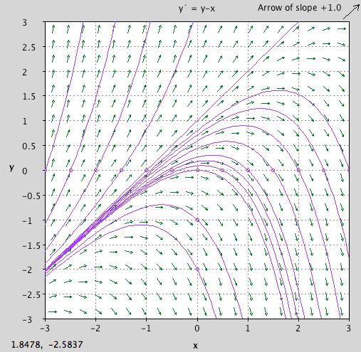
14
 c) Explain why each IVP has a solution, but this solution does not exist for all x.")
15 Exercise 3: Consider the differential equation dx = 1 y2. a) Use separation of variables to find solutions to this DE. b) Use the slope field below to sketch some solution graphs. Are your graphs consistent with the formulas from a? (You can sketch by hand, I'll use "dfield" on my browser.) c) Explain why each IVP has a solution, but this solution does not exist for all x. You can download the java applet "dfield" from the URL (You also have to download a toolkit, following the directions there.)
 Once we find these solutions, we can figure out why separation of variables missed them.")
16 Exercise 4a) Use separation of variables to solve the IVP dx = y y 0 = 0 4b) But there are actually a lot more solutions to this IVP! (Solutions which don't arise from the separation of variables algorithm are called singular solutions.) Once we find these solutions, we can figure out why separation of variables missed them. 4c) Sketch some of these singular solutions onto the slope field below. 2 3
17 Here's what's going on (stated in 1.3 page 24 of text; partly proven in Appendix A.) Existence - uniqueness theorem for the initial value problem Consider the IVP dx = f x, y y a = b Let the point a, b be interior to a coordinate rectangle R : a 1 x a 2, b 1 y b 2 in the x y plane. Existence: If f x, y is continuous in R (i.e. if two points in R are close enough, then the values of f at those two points are as close as we want). Then there exists a solution to the IVP, defined on some subinterval J a 1, a 2. Uniqueness: If the partial derivative function f x, y is also continuous in R, then for any y subinterval a J 0 J of x values for which the graph y = y x lies in the rectangle, the solution is unique! See figure below. The intuition for existence is that if the slope field f x, y is continuous, one can follow it from the initial point to reconstruct the graph. The condition on the y-partial derivative of f x, y turns out to prevent multiple graphs from being able to peel off. Exercise 5: Discuss how the existence-uniqueness theorem is consistent with our work in Exercises 1-4 in today's notes, where we were able to find explicit solution formulas because the differential equations were actually separable (#1,3,4) or when the solution formula was given to us (#2).
 Math 2250-004 Week 1 notes We will not necessarily finish the material from a given day's notes on that day. We may also add or subtract some material as the week progresses, but these notes represent
Math Week 1 notes
 Math 2250-004 Week 1 notes We will not necessarily finish the material from a given day's notes on that day. Or on an amazing day we may get farther than I've predicted. We may also add or subtract some
Exercise 4) Newton's law of cooling is a model for how objects are heated or cooled by the temperature of an ambient medium surrounding them.
 Newton's law of cooling is a model for how objects are heated or cooled by the temperature of an ambient medium surrounding them.") Exercise 4) Newton's law of cooling is a model for how objects are heated or cooled by the temperature of an ambient medium surrounding them. In this model, the bo temperature T = T t changes at a rate
Exercise 4) Newton's law of cooling is a model for how objects are heated or cooled by the temperature of an ambient medium surrounding them. In this model, the bo temperature T = T t changes at a rate
. If y x is a solution to this IVP and if we consider its graph y = y x, then the IC means the graph must pass through the point x 0
 Math 2250-004 Wed Jan 11 Quiz today at end of class, on section 1.1-1.2 material After finishing Tuesday's notes if necessary, begin Section 1.3: slope fields and graphs of differential equation solutions:
Exercise 4) Newton's law of cooling is a model for how objects are heated or cooled by the temperature of an ambient medium surrounding them.
 Newton's law of cooling is a model for how objects are heated or cooled by the temperature of an ambient medium surrounding them.") Exercise 4) Newton's law of cooling is a model for how objects are heated or cooled by the temperature of an ambient medium surrounding them. In this model, the body temperature T = T t changes at a rate
Exercise 4) Newton's law of cooling is a model for how objects are heated or cooled by the temperature of an ambient medium surrounding them. In this model, the body temperature T = T t changes at a rate
Section 1.3: slope fields and graphs of differential equation solutions: Consider the first order DE IVP for a function y x : y = f x, y, y x 0
 Section 1.3: slope fields and graphs of differential equation solutions: Consider the first order DE IVP for a function y x : y = f x, y, y x 0 = y 0. If y x is a solution to this IVP and if we consider
for the initial position and velocity. Find formulas for v t and x t. b) Assuming x 0 = 0 and v 0 O 0, show that the maximum value of x t is x max
 Assuming x 0 = 0 and v 0 O 0, show that the maximum value of x t is x max") Math 2250-4 Wed Aug 28 Finish 1.2. Differential equations of the form y# x = f x. Then begin section 1.3, slope fields., We still have two exercises to finish from Tuesday's notes: the formula for the
Math 2250-4 Wed Aug 28 Finish 1.2. Differential equations of the form y# x = f x. Then begin section 1.3, slope fields., We still have two exercises to finish from Tuesday's notes: the formula for the
Syllabus for Math Di erential Equations and Linear Algebra Spring 2018
 Syllabus for Math 2250-004 Di erential Equations and Linear Algebra Spring 2018 Instructor Professor Nick Korevaar email korevaar@math.utah.edu o ce LCB 204, 801.581.7318 o ce hours M 2:00-3:00 p.m. LCB
Mon Jan Improved acceleration models: linear and quadratic drag forces. Announcements: Warm-up Exercise:
 Math 2250-004 Week 4 notes We will not necessarily finish the material from a given day's notes on that day. We may also add or subtract some material as the week progresses, but these notes represent
Math Week 1 notes
 Math 2270-004 Week notes We will not necessarily finish the material from a given day's notes on that day. Or on an amazing day we may get farther than I've predicted. We may also add or subtract some
Solving Differential Equations: First Steps
 30 ORDINARY DIFFERENTIAL EQUATIONS 3 Solving Differential Equations Solving Differential Equations: First Steps Now we start answering the question which is the theme of this book given a differential
Finish section 3.6 on Determinants and connections to matrix inverses. Use last week's notes. Then if we have time on Tuesday, begin:
 Math 225-4 Week 7 notes Sections 4-43 vector space concepts Tues Feb 2 Finish section 36 on Determinants and connections to matrix inverses Use last week's notes Then if we have time on Tuesday, begin
Wed Feb The vector spaces 2, 3, n. Announcements: Warm-up Exercise:
 Wed Feb 2 4-42 The vector spaces 2, 3, n Announcements: Warm-up Exercise: 4-42 The vector space m and its subspaces; concepts related to "linear combinations of vectors" Geometric interpretation of vectors
Mon Jan Improved acceleration models: linear and quadratic drag forces. Announcements: Warm-up Exercise:
 Math 2250-004 Week 4 notes We will not necessarily finish the material from a given day's notes on that day. We may also add or subtract some material as the week progresses, but these notes represent
5.1 Second order linear differential equations, and vector space theory connections.
 Math 2250-004 Wed Mar 1 5.1 Second order linear differential equations, and vector space theory connections. Definition: A vector space is a collection of objects together with and "addition" operation
is any vector v that is a sum of scalar multiples of those vectors, i.e. any v expressible as v = c 1 v n ... c n v 2 = 0 c 1 = c 2
 Math 225-4 Week 8 Finish sections 42-44 and linear combination concepts, and then begin Chapter 5 on linear differential equations, sections 5-52 Mon Feb 27 Use last Friday's notes to talk about linear
7.1 Indefinite Integrals Calculus
 7.1 Indefinite Integrals Calculus Learning Objectives A student will be able to: Find antiderivatives of functions. Represent antiderivatives. Interpret the constant of integration graphically. Solve differential
Please read for extra test points: Thanks for reviewing the notes you are indeed a true scholar!
 Please read for extra test points: Thanks for reviewing the notes you are indeed a true scholar! See me any time B4 school tomorrow and mention to me that you have reviewed your integration notes and you
Disclaimer: This Final Exam Study Guide is meant to help you start studying. It is not necessarily a complete list of everything you need to know.
 Disclaimer: This is meant to help you start studying. It is not necessarily a complete list of everything you need to know. The MTH 132 final exam mainly consists of standard response questions where students
Examples: u = is a vector in 2. is a vector in 5.
 3 Vectors and vector equations We'll carefully define vectors, algebraic operations on vectors and geometric interpretations of these operations, in terms of displacements These ideas will eventually give
APPLICATIONS OF DIFFERENTIATION
 4 APPLICATIONS OF DIFFERENTIATION APPLICATIONS OF DIFFERENTIATION 4.9 Antiderivatives In this section, we will learn about: Antiderivatives and how they are useful in solving certain scientific problems.
Plane Curves and Parametric Equations
 Plane Curves and Parametric Equations MATH 211, Calculus II J. Robert Buchanan Department of Mathematics Spring 2018 Introduction We typically think of a graph as a curve in the xy-plane generated by the
AP Physics C Summer Homework. Questions labeled in [brackets] are required only for students who have completed AP Calculus AB
![AP Physics C Summer Homework. Questions labeled in [brackets] are required only for students who have completed AP Calculus AB](/thumbs/96/128301637.jpg "AP Physics C Summer Homework. Questions labeled in [brackets] are required only for students who have completed AP Calculus AB") 1. AP Physics C Summer Homework NAME: Questions labeled in [brackets] are required only for students who have completed AP Calculus AB 2. Fill in the radian conversion of each angle and the trigonometric
1. AP Physics C Summer Homework NAME: Questions labeled in [brackets] are required only for students who have completed AP Calculus AB 2. Fill in the radian conversion of each angle and the trigonometric
4 The Cartesian Coordinate System- Pictures of Equations
 4 The Cartesian Coordinate System- Pictures of Equations Concepts: The Cartesian Coordinate System Graphs of Equations in Two Variables x-intercepts and y-intercepts Distance in Two Dimensions and the
= L y 1. y 2. L y 2 (2) L c y = c L y, c.
 L c y = c L y, c.") Definition: A second order linear differential equation for a function y x is a differential equation that can be written in the form A x y B x y C x y = F x. We search for solution functions y x defined
Definition: A second order linear differential equation for a function y x is a differential equation that can be written in the form A x y B x y C x y = F x. We search for solution functions y x defined
Mon Jan Matrix and linear transformations. Announcements: Warm-up Exercise:
 Math 2270-004 Week 4 notes We will not necessarily finish the material from a given day's notes on that day. We may also add or subtract some material as the week progresses, but these notes represent
Unit IV Derivatives 20 Hours Finish by Christmas
 Unit IV Derivatives 20 Hours Finish by Christmas Calculus There two main streams of Calculus: Differentiation Integration Differentiation is used to find the rate of change of variables relative to one
Unit IV Derivatives 20 Hours Finish by Christmas
 Unit IV Derivatives 20 Hours Finish by Christmas Calculus There two main streams of Calculus: Differentiation Integration Differentiation is used to find the rate of change of variables relative to one
MATH 2554 (Calculus I)
") MATH 2554 (Calculus I) Dr. Ashley K. University of Arkansas February 21, 2015 Table of Contents Week 6 1 Week 6: 16-20 February 3.5 Derivatives as Rates of Change 3.6 The Chain Rule 3.7 Implicit Differentiation
MATH 2554 (Calculus I) Dr. Ashley K. University of Arkansas February 21, 2015 Table of Contents Week 6 1 Week 6: 16-20 February 3.5 Derivatives as Rates of Change 3.6 The Chain Rule 3.7 Implicit Differentiation
Advanced Higher Mathematics of Mechanics
 Advanced Higher Mathematics of Mechanics Course Outline (2016-2017) Block 1: Change of timetable to summer holiday Assessment Standard Assessment 1 Applying skills to motion in a straight line (Linear
The Fundamental Theorem of Calculus Part 3
 The Fundamental Theorem of Calculus Part FTC Part Worksheet 5: Basic Rules, Initial Value Problems, Rewriting Integrands A. It s time to find anti-derivatives algebraically. Instead of saying the anti-derivative
Learning Objectives for Math 165
 Learning Objectives for Math 165 Chapter 2 Limits Section 2.1: Average Rate of Change. State the definition of average rate of change Describe what the rate of change does and does not tell us in a given
Rolle s Theorem. The theorem states that if f (a) = f (b), then there is at least one number c between a and b at which f ' (c) = 0.
 = f (b), then there is at least one number c between a and b at which f ' (c) = 0.") Rolle s Theorem Rolle's Theorem guarantees that there will be at least one extreme value in the interior of a closed interval, given that certain conditions are satisfied. As with most of the theorems
Rolle s Theorem Rolle's Theorem guarantees that there will be at least one extreme value in the interior of a closed interval, given that certain conditions are satisfied. As with most of the theorems
First-Order Differential Equations
 CHAPTER 1 First-Order Differential Equations 1. Diff Eqns and Math Models Know what it means for a function to be a solution to a differential equation. In order to figure out if y = y(x) is a solution
WELCOME TO PHYSICS 201. Dr. Luis Dias Summer 2007 M, Tu, Wed, Th 10am-12pm 245 Walter Hall
 WELCOME TO PHYSICS 201 Dr. Luis Dias Summer 2007 M, Tu, Wed, Th 10am-12pm 245 Walter Hall PHYSICS 201 - Summer 2007 TEXTBOOK: Cutnell & Johnson, 6th ed. SYLLABUS : Please READ IT carefully. LONCAPA Learning
The real voyage of discovery consists not in seeking new landscapes, but in having new eyes. Marcel Proust
 The real voyage of discovery consists not in seeking new landscapes, but in having new eyes. Marcel Proust School of the Art Institute of Chicago Calculus Frank Timmes ftimmes@artic.edu flash.uchicago.edu/~fxt/class_pages/class_calc.shtml
Relationships Between Quantities
 Algebra 1 Relationships Between Quantities Relationships Between Quantities Everyone loves math until there are letters (known as variables) in problems!! Do students complain about reading when they come
Displacement and Total Distance Traveled
 Displacement and Total Distance Traveled We have gone over these concepts before. Displacement: This is the distance a particle has moved within a certain time - To find this you simply subtract its position
9.3: Separable Equations
 9.3: Separable Equations An equation is separable if one can move terms so that each side of the equation only contains 1 variable. Consider the 1st order equation = F (x, y). dx When F (x, y) = f (x)g(y),
Physics 20 Homework 2 SIMS 2016
 Physics 20 Homework 2 SIMS 2016 Due: Saturday, August 20 th 1. In class, we ignored air resistance in our discussion of projectile motion. Now, let s derive the relevant equation of motion in the case
4. Name the transformation needed to transform Figure A into Figure B, using one movement. l
 Review 1 Use the following words to fill in the blank to make true sentences. translation rotation reflection 1. A is a transformation that slides a figure a given distance in a given direction. 2. A is
Solutions to the Review Questions
 Solutions to the Review Questions Short Answer/True or False. True or False, and explain: (a) If y = y + 2t, then 0 = y + 2t is an equilibrium solution. False: This is an isocline associated with a slope
Math 106 Answers to Exam 3a Fall 2015
 Math 6 Answers to Exam 3a Fall 5.. Consider the curve given parametrically by x(t) = cos(t), y(t) = (t 3 ) 3, for t from π to π. (a) (6 points) Find all the points (x, y) where the graph has either a vertical
MAT137 - Term 2, Week 2
 MAT137 - Term 2, Week 2 This lecture will assume you have watched all of the videos on the definition of the integral (but will remind you about some things). Today we re talking about: More on the definition
It is convenient to think that solutions of differential equations consist of a family of functions (just like indefinite integrals ).
.") Section 1.1 Direction Fields Key Terms/Ideas: Mathematical model Geometric behavior of solutions without solving the model using calculus Graphical description using direction fields Equilibrium solution
Section 1.1 Direction Fields Key Terms/Ideas: Mathematical model Geometric behavior of solutions without solving the model using calculus Graphical description using direction fields Equilibrium solution
Numerical method for approximating the solution of an IVP. Euler Algorithm (the simplest approximation method)
") Section 2.7 Euler s Method (Computer Approximation) Key Terms/ Ideas: Numerical method for approximating the solution of an IVP Linear Approximation; Tangent Line Euler Algorithm (the simplest approximation
Section 2.7 Euler s Method (Computer Approximation) Key Terms/ Ideas: Numerical method for approximating the solution of an IVP Linear Approximation; Tangent Line Euler Algorithm (the simplest approximation
Unit #6 Basic Integration and Applications Homework Packet
 Unit #6 Basic Integration and Applications Homework Packet For problems, find the indefinite integrals below.. x 3 3. x 3x 3. x x 3x 4. 3 / x x 5. x 6. 3x x3 x 3 x w w 7. y 3 y dy 8. dw Daily Lessons and
Unit #3 Rules of Differentiation Homework Packet
 Unit #3 Rules of Differentiation Homework Packet In the table below, a function is given. Show the algebraic analysis that leads to the derivative of the function. Find the derivative by the specified
5.5 Deeper Properties of Continuous Functions
 5.5. DEEPER PROPERTIES OF CONTINUOUS FUNCTIONS 195 5.5 Deeper Properties of Continuous Functions 5.5.1 Intermediate Value Theorem and Consequences When one studies a function, one is usually interested
Chapter 5: Integrals
 Chapter 5: Integrals Section 5.3 The Fundamental Theorem of Calculus Sec. 5.3: The Fundamental Theorem of Calculus Fundamental Theorem of Calculus: Sec. 5.3: The Fundamental Theorem of Calculus Fundamental
UNIT I: MECHANICS Chapter 5: Projectile Motion
 IMPORTANT TERMS: Component Projectile Resolution Resultant Satellite Scalar quantity Vector Vector quantity UNIT I: MECHANICS Chapter 5: Projectile Motion I. Vector and Scalar Quantities (5-1) A. Vector
Chapter1. Ordinary Differential Equations
 Chapter1. Ordinary Differential Equations In the sciences and engineering, mathematical models are developed to aid in the understanding of physical phenomena. These models often yield an equation that
MATH1013 Calculus I. Introduction to Functions 1
 MATH1013 Calculus I Introduction to Functions 1 Edmund Y. M. Chiang Department of Mathematics Hong Kong University of Science & Technology May 9, 2013 Integration I (Chapter 4) 2013 1 Based on Briggs,
Integrals. D. DeTurck. January 1, University of Pennsylvania. D. DeTurck Math A: Integrals 1 / 61
 Integrals D. DeTurck University of Pennsylvania January 1, 2018 D. DeTurck Math 104 002 2018A: Integrals 1 / 61 Integrals Start with dx this means a little bit of x or a little change in x If we add up
Mon Feb Matrix algebra and matrix inverses. Announcements: Warm-up Exercise:
 Math 2270-004 Week 5 notes We will not necessarily finish the material from a given day's notes on that day We may also add or subtract some material as the week progresses, but these notes represent an
Welcome to. Elementary Calculus with Trig II CRN(13828) Instructor: Quanlei Fang. Department of Mathematics, Virginia Tech, Spring 2008
 Instructor: Quanlei Fang. Department of Mathematics, Virginia Tech, Spring 2008") Welcome to Elementary Calculus with Trig II CRN(13828) Instructor: Quanlei Fang Department of Mathematics, Virginia Tech, Spring 2008 1 Be sure to read the course contract Contact Information Text Grading
Welcome to Elementary Calculus with Trig II CRN(13828) Instructor: Quanlei Fang Department of Mathematics, Virginia Tech, Spring 2008 1 Be sure to read the course contract Contact Information Text Grading
equations that I should use? As you see the examples, you will end up with a system of equations that you have to solve
 Preface The common question is Which is the equation that I should use?. I think I will rephrase the question as Which are the equations that I should use? As you see the examples, you will end up with
CALCULUS AB SUMMER ASSIGNMENT
 CALCULUS AB SUMMER ASSIGNMENT Dear Prospective Calculus Students, Welcome to AP Calculus. This is a rigorous, yet rewarding, math course. Most of the students who have taken Calculus in the past are amazed
Antiderivatives. Definition A function, F, is said to be an antiderivative of a function, f, on an interval, I, if. F x f x for all x I.
 Antiderivatives Definition A function, F, is said to be an antiderivative of a function, f, on an interval, I, if F x f x for all x I. Theorem If F is an antiderivative of f on I, then every function of
Solutions to the Review Questions
 Solutions to the Review Questions Short Answer/True or False. True or False, and explain: (a) If y = y + 2t, then 0 = y + 2t is an equilibrium solution. False: (a) Equilibrium solutions are only defined
DIFFERENTIAL EQUATIONS
 DIFFERENTIAL EQUATIONS Basic Concepts Paul Dawkins Table of Contents Preface... Basic Concepts... 1 Introduction... 1 Definitions... Direction Fields... 8 Final Thoughts...19 007 Paul Dawkins i http://tutorial.math.lamar.edu/terms.aspx
5.3 Interpretations of the Definite Integral Student Notes
 5. Interpretations of the Definite Integral Student Notes The Total Change Theorem: The integral of a rate of change is the total change: a b F This theorem is used in many applications. xdx Fb Fa Example
Announcements Monday, September 25
 Announcements Monday, September 25 The midterm will be returned in recitation on Friday. You can pick it up from me in office hours before then. Keep tabs on your grades on Canvas. WeBWorK 1.7 is due Friday
Sample Questions, Exam 1 Math 244 Spring 2007
 Sample Questions, Exam Math 244 Spring 2007 Remember, on the exam you may use a calculator, but NOT one that can perform symbolic manipulation (remembering derivative and integral formulas are a part of
Math 308, Sections 301, 302, Summer 2008 Review before Test I 06/09/2008
 Math 308, Sections 301, 302, Summer 2008 Review before Test I 06/09/2008 Chapter 1. Introduction Section 1.1 Background Definition Equation that contains some derivatives of an unknown function is called
AP Calculus BC Syllabus
 AP Calculus BC Syllabus Course Overview AP Calculus BC is the study of the topics covered in college-level Calculus I and Calculus II. This course includes instruction and student assignments on all of
6.2 Deeper Properties of Continuous Functions
 6.2. DEEPER PROPERTIES OF CONTINUOUS FUNCTIONS 69 6.2 Deeper Properties of Continuous Functions 6.2. Intermediate Value Theorem and Consequences When one studies a function, one is usually interested in
MAT137 - Term 2, Week 4
 MAT137 - Term 2, Week 4 Reminders: Your Problem Set 6 is due tomorrow at 3pm. Test 3 is next Friday, February 3, at 4pm. See the course website for details. Today we will: Talk more about substitution.
For those of you who are taking Calculus AB concurrently with AP Physics, I have developed a
 AP Physics C: Mechanics Greetings, For those of you who are taking Calculus AB concurrently with AP Physics, I have developed a brief introduction to Calculus that gives you an operational knowledge of
Differential Equations Spring 2007 Assignments
 Differential Equations Spring 2007 Assignments Homework 1, due 1/10/7 Read the first two chapters of the book up to the end of section 2.4. Prepare for the first quiz on Friday 10th January (material up
Final Exam Review. MATH Intuitive Calculus Fall 2013 Circle lab day: Mon / Fri. Name:. Show all your work.
 MATH 11012 Intuitive Calculus Fall 2013 Circle lab day: Mon / Fri Dr. Kracht Name:. 1. Consider the function f depicted below. Final Exam Review Show all your work. y 1 1 x (a) Find each of the following
Spring 2015, Math 111 Lab 4: Kinematics of Linear Motion
 Spring 2015, Math 111 Lab 4: William and Mary February 24, 2015 Spring 2015, Math 111 Lab 4: Learning Objectives Today, we will be looking at applications of derivatives in the field of kinematics. Learning
AP Calculus BC Syllabus
 Instructor: Jennifer Manzano-Tackett jennifer-manzano@scusd.edu (916) 395-5090 Ext. 506308 www.mt-jfk.com AP Calculus BC Syllabus Textbook: Calculus, 6th edition, by Larson, Hostetler and Edwards: Houghton
Acceleration and Force: I
 Lab Section (circle): Day: Monday Tuesday Time: 8:00 9:30 1:10 2:40 Acceleration and Force: I Name Partners Pre-Lab You are required to finish this section before coming to the lab, which will be checked
Theorem 3: The solution space to the second order homogeneous linear differential equation y p x y q x y = 0 is 2-dimensional.
 Unlike in the previous example, and unlike what was true for the first order linear differential equation y p x y = q x there is not a clever integrating factor formula that will always work to find the
AP Calculus BC. Course Overview. Course Outline and Pacing Guide
 AP Calculus BC Course Overview AP Calculus BC is designed to follow the topic outline in the AP Calculus Course Description provided by the College Board. The primary objective of this course is to provide
1 Antiderivatives graphically and numerically
 Math B - Calculus by Hughes-Hallett, et al. Chapter 6 - Constructing antiderivatives Prepared by Jason Gaddis Antiderivatives graphically and numerically Definition.. The antiderivative of a function f
New Material Section 1: Functions and Geometry occurring in engineering
 New Material Section 1: Functions and Geometry occurring in engineering 1. Plotting Functions: Using appropriate software to plot the graph of a function Linear f(x) = mx+c Quadratic f(x) = Px +Qx+R Cubic
Chapter 6: The Definite Integral
 Name: Date: Period: AP Calc AB Mr. Mellina Chapter 6: The Definite Integral v v Sections: v 6.1 Estimating with Finite Sums v 6.5 Trapezoidal Rule v 6.2 Definite Integrals 6.3 Definite Integrals and Antiderivatives
Name Period Date. polynomials of the form x ± bx ± c. Use guess and check and logic to factor polynomials of the form 2
 Name Period Date POLYNOMIALS Student Packet 3: Factoring Polynomials POLY3 STUDENT PAGES POLY3.1 An Introduction to Factoring Polynomials Understand what it means to factor a polynomial Factor polynomials
Numerical method for approximating the solution of an IVP. Euler Algorithm (the simplest approximation method)
") Section 2.7 Euler s Method (Computer Approximation) Key Terms/ Ideas: Numerical method for approximating the solution of an IVP Linear Approximation; Tangent Line Euler Algorithm (the simplest approximation
Section 2.7 Euler s Method (Computer Approximation) Key Terms/ Ideas: Numerical method for approximating the solution of an IVP Linear Approximation; Tangent Line Euler Algorithm (the simplest approximation
Math 180 Written Homework Assignment #10 Due Tuesday, December 2nd at the beginning of your discussion class.
 Math 18 Written Homework Assignment #1 Due Tuesday, December 2nd at the beginning of your discussion class. Directions. You are welcome to work on the following problems with other MATH 18 students, but
CHAPTER 1. First-Order Differential Equations and Their Applications. 1.1 Introduction to Ordinary Differential Equations
 CHAPTER 1 First-Order Differential Equations and Their Applications 1.1 Introduction to Ordinary Differential Equations Differential equations are found in many areas of mathematics, science, and engineering.
Tues Feb Vector spaces and subspaces. Announcements: Warm-up Exercise:
 Math 2270-004 Week 7 notes We will not necessarily finish the material from a given day's notes on that day. We may also add or subtract some material as the week progresses, but these notes represent
( ) be the particular solution to the differential equation passing through the point (2, 1). Write an
 be the particular solution to the differential equation passing through the point (2, 1). Write an") 70. AB Calculus Step-by-Step Name Consider the differential equation dy dx = x +1 y. ( ) be the particular solution to the differential equation passing through the point (2, 1). Write an a. Let f x equation
70. AB Calculus Step-by-Step Name Consider the differential equation dy dx = x +1 y. ( ) be the particular solution to the differential equation passing through the point (2, 1). Write an a. Let f x equation
The acceleration of gravity is constant (near the surface of the earth). So, for falling objects:
. So, for falling objects:") 1. Become familiar with a definition of and terminology involved with differential equations Calculus - Santowski. Solve differential equations with and without initial conditions 3. Apply differential
1. Become familiar with a definition of and terminology involved with differential equations Calculus - Santowski. Solve differential equations with and without initial conditions 3. Apply differential
Review. The derivative of y = f(x) has four levels of meaning: Physical: If y is a quantity depending on x, the derivative dy
 has four levels of meaning: Physical: If y is a quantity depending on x, the derivative dy") Math 132 Area and Distance Stewart 4.1/I Review. The derivative of y = f(x) has four levels of meaning: Physical: If y is a quantity depending on x, the derivative dy dx x=a is the rate of change of y
Math 132 Area and Distance Stewart 4.1/I Review. The derivative of y = f(x) has four levels of meaning: Physical: If y is a quantity depending on x, the derivative dy dx x=a is the rate of change of y
5.3 Definite Integrals and Antiderivatives
 5.3 Definite Integrals and Antiderivatives Objective SWBAT use properties of definite integrals, average value of a function, mean value theorem for definite integrals, and connect differential and integral
1abcdef, 9, 10, 17, 20, 21, (in just do parts a, b and find domains)
") Sample Homework from Dr. Steve Merrin Math 1210 Calculus I Text: Calculus by James Stewart, 8th edition Chapter 1 sec 1.1 Some algebra review 3, 7, 8, 25, 27, 29-35, 38, 41, 43, 44, 63 Students should
Sample Homework from Dr. Steve Merrin Math 1210 Calculus I Text: Calculus by James Stewart, 8th edition Chapter 1 sec 1.1 Some algebra review 3, 7, 8, 25, 27, 29-35, 38, 41, 43, 44, 63 Students should
Topics Covered in Calculus BC
 Topics Covered in Calculus BC Calculus BC Correlation 5 A Functions, Graphs, and Limits 1. Analysis of graphs 2. Limits or functions (including one sides limits) a. An intuitive understanding of the limiting
Daily Lessons and Assessments for AP* Calculus AB, A Complete Course Page 584 Mark Sparks 2012
 The Second Fundamental Theorem of Calculus Functions Defined by Integrals Given the functions, f(t), below, use F( ) f ( t) dt to find F() and F () in terms of.. f(t) = 4t t. f(t) = cos t Given the functions,
Pre-Calc Chapter 1 Sample Test. D) slope: 3 4
 slope: 3 4") Pre-Calc Chapter 1 Sample Test 1. Use the graphs of f and g to evaluate the function. f( x) gx ( ) (f o g)(-0.5) 1 1 0 4. Plot the points and find the slope of the line passing through the pair of points.
Pre-Calc Chapter 1 Sample Test 1. Use the graphs of f and g to evaluate the function. f( x) gx ( ) (f o g)(-0.5) 1 1 0 4. Plot the points and find the slope of the line passing through the pair of points.
MATH 3A FINAL REVIEW
 MATH 3A FINAL REVIEW Guidelines to taking the nal exam You must show your work very clearly You will receive no credit if we do not understand what you are doing 2 You must cross out any incorrect work
Math 416, Spring 2010 More on Algebraic and Geometric Properties January 21, 2010 MORE ON ALGEBRAIC AND GEOMETRIC PROPERTIES
 Math 46, Spring 2 More on Algebraic and Geometric Properties January 2, 2 MORE ON ALGEBRAIC AND GEOMETRIC PROPERTIES Algebraic properties Algebraic properties of matrix/vector multiplication Last time
MITOCW ocw f99-lec01_300k
 MITOCW ocw-18.06-f99-lec01_300k Hi. This is the first lecture in MIT's course 18.06, linear algebra, and I'm Gilbert Strang. The text for the course is this book, Introduction to Linear Algebra. And the
MATH 250 TOPIC 13 INTEGRATION. 13B. Constant, Sum, and Difference Rules
 Math 5 Integration Topic 3 Page MATH 5 TOPIC 3 INTEGRATION 3A. Integration of Common Functions Practice Problems 3B. Constant, Sum, and Difference Rules Practice Problems 3C. Substitution Practice Problems
Practice problems from old exams for math 132 William H. Meeks III
 Practice problems from old exams for math 32 William H. Meeks III Disclaimer: Your instructor covers far more materials that we can possibly fit into a four/five questions exams. These practice tests are
Introduction to First Order Equations Sections
 A B I L E N E C H R I S T I A N U N I V E R S I T Y Department of Mathematics Introduction to First Order Equations Sections 2.1-2.3 Dr. John Ehrke Department of Mathematics Fall 2012 Course Goals The
Motion in Space. MATH 311, Calculus III. J. Robert Buchanan. Fall Department of Mathematics. J. Robert Buchanan Motion in Space
 Motion in Space MATH 311, Calculus III J. Robert Buchanan Department of Mathematics Fall 2011 Background Suppose the position vector of a moving object is given by r(t) = f (t), g(t), h(t), Background
Chapter 5: Integrals
 Chapter 5: Integrals Section 5.5 The Substitution Rule (u-substitution) Sec. 5.5: The Substitution Rule We know how to find the derivative of any combination of functions Sum rule Difference rule Constant