Ordinary Differential Equations

Transcription

1 12/01/2015

2 Table of contents Second Order Differential Equations Higher Order Differential Equations Series The Laplace Transform System of First Order Linear Differential Equations Nonlinear Differential Equations

3 Definitions Classification Basic Examples Direction Fields Figure: Sophus Lie.

4 Definitions Classification Basic Examples Direction Fields Definitions Differential Equations A differential equation is any equation which contains derivatives, either ordinary or partial derivatives. There many situations where we ca find such an object. Thus, for instance in the case of the study of Classical Mechanics in Physics, if an object of mass m is moving with acceleration a and being acted on with force F then Newtons Second Law tells us. F = ma

5 Definitions Classification Basic Examples Direction Fields Definitions To see that this is in fact a differential equation. First, remember that we can rewrite the acceleration, a, in one of two ways. a = dv or a = d 2 u dt dt 2 Where v is the velocity of the object and u is the position function of the object at any time t. We should also remember at this point that the force, F may also be a function of time, velocity, and/or position. m dv dt = F (t, v) or m d 2 u = F (t, u, v) dt2

6 Definitions Classification Basic Examples Direction Fields Definitions More examples of differential equations 2y + 3y 5y = 0 cos(y) d 2 y (1 + y)dy dx 2 dx + y 3 e y = 0 y (4) + 5y 4y + y = sin(x) a 2 2 u x 2 = u t a 2 2 u x 2 = 2 u t 2 u 3 2 x t = 1 + u y

7 Definitions Classification Basic Examples Direction Fields Definitions Solution A solution to a differential equation on an interval α < t < β is any function y(t) which satisfies the differential equation in question on the interval. It is important to note that the solutions are often accompanied by intervals and these intervals can impart some important information about the solution.

8 Definitions Classification Basic Examples Direction Fields Classification Order The order of a differential equation is the largest derivative present in the differential equation. The equation m dv = F (t, v) dt is a first order differential equation, the equations m d 2 u = F (t, u, v) dt2 2y + 3y 5y = 0 cos(y) d 2 y (1 + y)dy dx 2 dx + y 3 e y = 0

9 Definitions Classification Basic Examples Direction Fields Classification a 2 2 u x 2 = u t a 2 2 u x 2 = 2 u t 2 are second order differential equations, the equation u 3 2 x t = 1 + u y is a third order differential equation and finally, the equation y (4) + 5y 4y + y = sin(x) is a fourth order differential equation.

10 Definitions Classification Basic Examples Direction Fields Classification Note that the order does not depend on whether or not you ve got ordinary or partial derivatives in the differential equation. As you will see most of the solution techniques for second order differential equations can be easily (and naturally) extended to higher order differential equations. Ordinary and Partial Differential Equations A differential equation is called an ordinary differential equation, abbreviated by ODE, if it has ordinary derivatives in it. Likewise, a differential equation is called a partial differential equation, abbreviated by PDE, if it has partial derivatives in it.

11 Definitions Classification Basic Examples Direction Fields Classification Linear Differential Equations A linear differential equation is any differential equation that can be written in the following form. a n (t)y (n) + a n 1 (t)y (n 1) a 1 (t)y + a 0 (t)y = g(t) The important thing to note about linear differential equations is that there are no products of the function, y(t), and its derivatives and neither the function or its derivatives occur to any power other than the first power.

12 Definitions Classification Basic Examples Direction Fields Classification The coefficients a n (t),..., a 0 (t), g(t) can be any function. Only the function y(t) and its derivatives are used in determining if a differential equation is linear. If a differential equation cannot be written in the above form, then it is called a non-linear differential equation. In the examples above only cos(y) d 2 y (1 + y)dy dx 2 dx + y 3 e y = 0 is a non-linear equation. We can t classify Newton s Second Law equations since we do not know what form the function F has. These could be either linear or non-linear depending on F.

13 Definitions Classification Basic Examples Direction Fields Basic Examples Differential Equations in Physics Schrodinger s Equation. 2 2m 2 Ψ + V (r)ψ = i Ψ t Is the starting point for non-relativistic Quantum Mechanics, here the solution Ψ( r, t) is the wave function.

14 Definitions Classification Basic Examples Direction Fields Basic Examples Maxwell s equations: Ē = ρ ɛ 0, (1a) B = 0, Ē = B t, (1b) (1c) B = µ 0 ɛ 0 Ē t + µ 0 J, (1d) This is the set of fundamental equations for Classical Electromagnetism, here the solutions Ē and B represent the electrical and magnetic fields.

15 Definitions Classification Basic Examples Direction Fields Basic Examples Newton s Second Law. m d 2 r dt 2 = F ( r, t) Is the fundamental equation for Classical Mechanics, here the solution r(t) is the position as a function of time.

16 Definitions Classification Basic Examples Direction Fields Basic Examples Example 1 Show that y(x) = x 3/2 is a solution to 4x 2 y + 12xy + 3y = 0 for x > 0. Solution We will need the first and second derivatives : y (x) = 3 2 x 5/2, y (x) = 15 4 x 7/2 Plug these as well as the function into the differential equation:

17 Definitions Classification Basic Examples Direction Fields Basic Examples 4x 2 ( 15 4 x 7/2 ) + 12x( 3 2 x 5/2 ) + 3x 3/2 = 0 15x 3/2 18x 3/2 + 3x 3/2 = 0 0 = 0 So, y(x) = x 3/2 does satisfy the differential equation and hence is a solution. Why then didn t I include the condition that x > 0? I did not use this condition anywhere in the work showing that the function would satisfy the differential equation.

18 Definitions Classification Basic Examples Direction Fields Basic Examples To see why recall that y(x) = x 3/2 = 1 x 3/2 In this form it is clear that we will need to avoid x = 0 at the least as this would give division by zero. So, we saw in the last example that even though a function may symbolically satisfy a differential equation, because of certain restrictions brought about by the solution we cannot use all values of the independent variable and hence, must make a restriction on the independent variable.

19 Definitions Classification Basic Examples Direction Fields Basic Examples In the last example, note that there are in fact many more possible solutions to the differential equation. For instance all of the following are also solutions y(x) = x 1/2 y(x) = 5x 3/2 y(x) = 3x 1/2 y(x) = 2x 1/2 + 3x 3/2

20 Definitions Classification Basic Examples Direction Fields Basic Examples I ll leave the details to you to check that these are in fact solutions. Given these examples can you come up with any other solutions to the differential equation? y(x) = c 1 x 1/2 + c 2 x 3/2 There are in fact an infinite number of solutions to this differential equation. So, given that there are an infinite number of solutions to the differential equation in the last example, we can ask a natural question. Which is the solution that we want or does it matter which solution we use? This question leads us to the next material in this section.

21 Definitions Classification Basic Examples Direction Fields Basic Examples Example 2 Show that y(x) = x 3/2 is a solution to 4x 2 y + 12xy + 3y = 0 with initial conditions y(4) = 1 8 and y (4) = Solution As we saw in previous example the function y(x) = x 3/2 is a solution and we can then note that y(4) = 4 3/2 = 1 4 3/2 = 1 8 y (4) = /2 = /2 = 3 64 and so this solution also meets the initial conditions.

22 Definitions Classification Basic Examples Direction Fields Basic Examples In fact, y(x) = x 3/2 is the only solution to this differential equation that satisfies these two initial conditions. Initial Value Problem An Initial Value Problem (or IVP) is a differential equation along with an appropriate number of initial conditions. Example 3 The following is an IVP 4x 2 y + 12xy + 3y = 0, y(4) = 1 8, and y (4) = 3 64.

23 Definitions Classification Basic Examples Direction Fields Basic Examples Example 4 This is another IVP 2ty + 4y = 3, y(1) = 4. As you can notice, the number of initial conditions required will depend on the order of the differential equation. Interval of Validity The interval of validity for an IVP with initial condition(s). y(t 0 ) = y 0, y (t 0 ) = y 1,..., y k (t 0 ) = y k

24 Definitions Classification Basic Examples Direction Fields Basic Examples is the largest possible interval on which the solution is valid and contains t 0. These are easy to define, but can be difficult to find in the practice. General Solution The general solution to a differential equation is the most general form that the solution can take and doesn t take any initial conditions into account.

25 Definitions Classification Basic Examples Direction Fields Basic Examples Example 5 y(t) = c t 2 is the general solution to 2ty + 4y = 3 Check it out!!!!!! In fact, all solutions to this differential equation will be in this form. This is one of the first differential equations that we will learn how to solve and we will be able to verify this shortly.

26 Definitions Classification Basic Examples Direction Fields Basic Examples Particular Solution The particular solution to a differential equation is the specific solution that not only satisfies the differential equation, but also satisfies the given initial condition(s). Example 6 What is the particular solution to the following IVP? 2ty + 4y = 3 y(1) = 4

27 Definitions Classification Basic Examples Direction Fields Basic Examples Solution This is actually easier to do than it might at the general solution is of the form: y(t) = c t 2 All what we need is to determine the value of c that will give us the solution that we are after. To find this, all we need to do is use our initial condition as follows: 4 = c 1 2

28 Definitions Classification Basic Examples Direction Fields Basic Examples c = = 19 4 So, the particular solution to the IVP is: y(t) = t 2

29 Definitions Classification Basic Examples Direction Fields Basic Examples Implicit/Explicit Solution An explicit solution is any solution that is given in the form y = y(t). An implicit solution is any solution that is not in explicit form, that is, y can not be expressed explicitely as a function of t. Note that it is possible to have either general implicit/explicit solutions and particular implicit/explicit solutions. Example 7 Show that y 2 = t 2 3 is an implicit solution of the differential equation yy = t.

30 Definitions Classification Basic Examples Direction Fields Basic Examples Solution Using implicit derivation, the solution follows: 2yy = 2t + 0 yy = t Example 8 Find a particular explicit solution to the IVP yy = t y(2) = 1

31 Definitions Classification Basic Examples Direction Fields Basic Examples Solution We already know from the previous example that an implicit solution to this IVP is y 2 = t 2 3. To find the explicit solution all we need to do is solve for y(t) from y(t) = ± t 2 3 Now, we ve got a problem here. There are two functions here and we only want one and in fact only one will be correct! We can determine the correct function by reapplying the initial condition.

32 Definitions Classification Basic Examples Direction Fields Basic Examples Only one of them will satisfy the initial condition. In this case we can see that the negative solution, will be the correct one. The explicit solution is then y(t) = t 2 3 In this case we were able to find an explicit solution to the differential equation. It should be noted however that it will not always be possible to find an explicit solution.

33 Definitions Classification Basic Examples Direction Fields Direction Fields There will be some situations where the ODE can be written in the form y = f (t, y) in such a way that to every point (t 0, y 0 ) that is in the domain of f on the Cartesian Plane we can assign a unique number y = f (t 0, y 0 ) called the Direction Field.

34 Definitions Classification Basic Examples Direction Fields Direction Fields It is clear that this construction is giving to us a geometrical approach to the solution of the equation since the Direction Field gives the slope of the tangent line of the solution curve. Thus, for example we have in the cases y = 1 y = t y = y y = t 2 + y 2 The Direction Fields are given by

35 Definitions Classification Basic Examples Direction Fields Direction Fields

36 Definitions Classification Basic Examples Direction Fields Direction Fields

37 Definitions Classification Basic Examples Direction Fields Direction Fields

38 Definitions Classification Basic Examples Direction Fields Direction Fields t2+y2.jpg

39 Definitions Classification Basic Examples Direction Fields Direction Fields And some solutions are plotted here

40 Definitions Classification Basic Examples Direction Fields Direction Fields

41 Definitions Classification Basic Examples Direction Fields Direction Fields

42 Definitions Classification Basic Examples Direction Fields Direction Fields The process of describing a physical situation with a differential equation is called modeling. We will be looking at modeling several times throughout this class. One of the simplest physical situations to think of is a falling object. So lets consider a falling object with mass m and derive a differential equation that, when solved, will give us the velocity of the object at any time, t. We will assume that only gravity and air resistance will act upon the object as it falls. Below is a figure showing the forces that will act upon the object.

43 Definitions Classification Basic Examples Direction Fields Direction Fields Now, lets take a look at the forces shown in the diagram above. F G is the force due to gravity and is given by F G = mg where g is the acceleration due to gravity. In this class we use g = 9.8m/s2 or g = 32ft/s2 depending on whether we will use the metric or British system.

44 Definitions Classification Basic Examples Direction Fields Direction Fields F A is the force due to air resistance and for this example we will assume that it is proportional to the velocity, v, of the mass. Therefore the force due to air resistance is then given by F A = γv, where γ > 0. Both y and v are positive and the force is acting upward. Recall from the previous section that Newtons Second Law of motion can be written as m dv dt = F (t, v)

45 Definitions Classification Basic Examples Direction Fields Direction Fields where F (t, v) is the sum of forces that act on the object and may be a function of the time t and the velocity of the object, v. For our situation we will have two forces acting on the object gravity,f G = mg, acting in the downward direction and hence will be positive, and air resistance, F A = γv, acting in the upward direction and hence will be negative. Putting all of this together into Newtons Second Law gives the following or m dv dt = mg γv

46 Definitions Classification Basic Examples Direction Fields Direction Fields dv dt = g γv m In order to look at direction fields, it would be helpful to have some numbers for the various quantities in the differential equation. So, let s assume that we have a mass of 2 kg and that γ = Plugging this into above gives the following differential equation. m dv = v dt whose direction field is given by

47 Definitions Classification Basic Examples Direction Fields Direction Fields

48 Definitions Classification Basic Examples Direction Fields Direction Fields So, just why do we care about direction fields? There are two nice pieces of information that can be readily found from the direction field for a differential equation. Sketch of solutions. Since the arrows in the direction fields are in fact tangents to the actual solutions to the differential equations we can use these as guides to sketch the graphs of solutions to the differential equation. Long Term Behavior. In many cases we are interested in how the solutions behave as t increases. Direction fields, if we can get our hands on them, can be used to find information about this long term behavior of the solution.

49 Definitions Classification Basic Examples Direction Fields Direction Fields Thus, in the case of a falling body we have that the long-term behavior can be seen from

50 Definitions Classification Basic Examples Direction Fields Direction Fields Another example is dy dt = (y 2 y 2)(1 y) 2. Whose direction field is

51 Definitions Classification Basic Examples Direction Fields Direction Fields An solutions are given by

52 Definitions Classification Basic Examples Direction Fields Direction Fields Finally, we have the next example dy dt = et 2y. Whose direction field and some solutions are

53

54 The first special case of first order differential equations that we will look is the linear first order differential equation. a(t)y + b(t)y = c(t) with a(t), b(t), and c(t) continuous function on some interval. Example 1 (4 + t 2 ) dy dt + 2ty = 4t

55 Solution d ( (4 + t 2 )y ) = 4t dt (4 + t 2 )y = 4tdt + C; C = constant y = (4 + t 2 )y = 2t 2 + C 2t2 (4 + t 2 ) + C (4 + t 2 )

56 In order to solve a linear first order differential equation we MUST start with the differential equation in the form shown below: dy + p(t)y = g(t) dt Where both p(t) and g(t) are continuous functions. If the differential equation is not in this form then the process we are going to use will not work.

57 Now, we are going to assume that there is some function somewhere out there, µ(t), called an integrating factor, such that, when we multiply the equation by it : µ(t) dy + µ(t)p(t)y = µ(t)g(t) dt that function has the property that µ(t)p(t) = µ (t)

58 And in this way the ODE becomes µ(t) dy dt + µ (t)y = µ(t)g(t) and using the product rule we obtain (µ(t)y(t)) = µ(t)g(t) Integrating and solving for y, we have y(t) = 1 ( ) µ(t)g(t)dt + C ; C = constant µ

59 So, now that weve got a general solution to a linear first order we need to go back and determine just what this function µ(t) is. This is actually an easier process. We will start with µ (t) = µ(t)p(t) µ (t) µ(t) = p(t) ln (µ(t)) = p(t)

60 Integrating, we obtain lnµ(t) = p(t)dt + K Exponentiate both sides to get µ(t) out of the natural logarithm. µ(t) = e p(t)dt+k

61 Now, let s make use of the fact that K is an unknown constant. If K is an unknown constant then so is e K, so we might as well just rename it k and make our life easier. This will give us the following. µ(t) = ke p(t)dt So, we now have a formula for the general solution of the linear first order differential equation, and a formula for the integrating factor.

62 We do have a problem however. We ve got two unknown constants and the more unknown constants we have the more trouble we will have later on. Therefore, it would be nice if we could find a way to eliminate one of them (we will not be able to eliminate both???). This is actually quite easy to do: ( ) 1 y(t) = p(t)dt ke g(t)dt + C ; C = constant y(t) = ke p(t)dt 1 ke p(t)dt ( k ) p(t)dt e g(t)dt + C ; C = constant

63 y(t) = y(t) = 1 e p(t)dt 1 e p(t)dt ( ( e p(t)dt g(t)dt + C ) ; C = constant k ) p(t)dt e g(t)dt + c ; c = constant The solution to a linear first order differential equation is then y(t) = 1 ( ) µ(t)g(t)dt + c ; c = constant µ where µ(t) = e p(t)dt

64 Now, we will need to use the integrating factor µ(t) regularly, as that formula is easier to use than the process to derive it. Solution Process The solution process for a first order linear differential equation is as follows. 1.- Put the linear differential equation in the correct initial form. dy dt + p(t)y(t) = g(t)

65 2.-Find the integrating factor µ(t). µ(t) = e p(t)dt 3.- Multiply everything in the differential equation by µ(t) and verify that the left side becomes the product rule (µ(t)y(t)) and write it as such. 4.- Integrate both sides, make sure you properly deal with the constant of integration. 5.- Solve for the solution y(t).

66 Example 2 Find the solution to the following differential equation: dv = v dt First we need to get the differential equation in the correct form: dv v(t) = 9.8 dt From this we can see that p(t) = and so µ(t) is then. µ(t) = e 0.196dt = e 0.196t

67 Multiply everything in the differential equation by µ(t) : 0.196t dv e dt + e0.196t 0.196v(t) = 9.8e 0.196t ( e 0.196t v(t) ) = 9.8e 0.196t Integrate both sides, make sure you properly deal with the constant of integration. (e 0.196t v(t) ) dt = 9.8e 0.196t dt

68 e 0.196t v(t) = 9.8e 0.196t dt and integrating e 0.196t v(t) = e0.196t + c Solve for the solution y(t). v(t) = 50 + ce 0.196t

69 From the solution to this example we can now see why the constant of integration is so important in this process. Without it, in this case, we would get a single, constant solution, v(t) = 50. With the constant of integration we get infinitely many solutions, one for each value of c. To sketch some solutions, all we need to do is to pick different values of c. Several of these are shown in the graph below:

70

71 Now, recall from the previous definitions that the Initial Condition(s) will allow us to pick particular solution. Solutions to first order differential equations (not just linear as we will see) will have a single unknown constant in them and so we will need exactly one initial condition to find the value of that constant and hence find the solution that we were after. The initial condition for first order differential equations will be of the form y(t 0 ) = y 0

72 Recall as well, that a differential equation along with a sufficient number of initial conditions is called an Initial Value Problem (IVP). Example 3 Solve the following IVP dv = v, v(0) = 48 dt To find the solution to an IVP, we must first find the general solution to the differential equation and then use the initial conditions to identify the exact solution that we are after.

73 So, since this is the same differential equation as we looked at in Example 2, we already have its general solution. v(t) = 50 + ce 0.196t And applying the initial conditions we have 48 = 50 + ce ( 0.196)(0) 48 = 50 + c c = 2

74 So, the actual solution to the IVP is: v(t) = 50 2e ( 0.196)(t)

75 Example 4 Solve the following IVP: cos(x)y +sin(x)y = 2cos 3 (x)sin(x) 1; y( π 4 ) = x < 2 Solution Rewrite the differential equation to get the coefficient of the derivative a one. y + sin(x) cos(x) y = 2cos2 (x)sin(x) 1 cos(x) y + tan(x)y = 2cos 2 (x)sin(x) sec(x)

76 Now find the integrating factor: µ(x) = e tanxdx = e ln secx = e lnsecx = secx Multiply the integrating factor through the differential equation and verify the left side is a product rule. sec(x)y + sec(x)tan(x)y = 2cos 2 (x)sin(x)sec(x) sec 2 (x) (sec(x)y(x)) = 2cos(x)sin(x) sec 2 (x) sec(x)y(x) = (2cos(x)sin(x) sec 2 (x) ) dx

77 sec(x)y(x) = (sin(2x) sec 2 (x) ) dx sec(x)y(x) = 1 cos(2x) tan(x) + c 2 y(x) = 1 cos(2x) 2 sec(x) tan(x) sec(x) + c sec(x) y(x) = 1 cos(2x) sin(x) + ccos(x) 2 sec(x)

78 Finally, apply the initial condition to find the value of c. 3 2 = y( π 4 ) = 1 cos( π 2 ) 2 sec( π 4 ) sin(π 4 ) + ccos(π 4 ) = 2 + c 2 c = 7 The solution is then y(x) = 1 cos(2x)cos(x) sin(x) + 7cos(x) 2

79 Below is a plot of the solution.

80 Example 5 Find the solution to the following IVP. Solution ty + 2y = t 2 t + 1; y(1) = 1 2 First, divide through by the t to get the differential equation into the correct form. y + 2 t y = t t

81 Now find the integrating factor: 2 µ(t) = e t dt = e 2ln t = e ln t2 = e lnt2 = t 2 Now, multiply the rewritten differential equation by the integrating factor. ( t 2 y ) = t 3 t 2 + t

82 Integrate both sides and solve for the solution. ( t 2 y ) (t = 3 t 2 + t ) dt t 2 y = t4 4 t3 3 + t2 2 + c y = t2 4 t c t 2

83 And applying initial conditions 1 2 = y(1) = c c = 1 12 The solution is then, y = t2 4 t t 2

84 Here is a plot of the solution.

85 Example 6 Find the solution to the following IVP. ty 2y = t 5 sin(2t) t 3 + 4t 4 ; y(π) = 3 2 (π))4 Solution First, divide through by the t to get the differential equation into the correct form. y 2 t y = t4 sin(2t) t 2 + 4t 3

86 Now find the integrating factor: µ(t) = e 2 t dt = e 2ln t = e ln t2 = e lnt2 = 1 t 2 Now, multiply the rewritten differential equation by the integrating factor. 1 t 2 y 1 2 t 2 t y = 1 ( t 4 t 2 sin(2t) t 2 + 4t 3) ( t 2 y ) = t 2 sin(2t) 1 + 4t

87 Integrate both sides and solve for the solution. ( t 2 y ) (t = 2 sin(2t) 1 + 4t ) dt t 2 y = t 2 sin(2t)dt dt + 4tdt t 2 y = 1 2 t2 cos(2t) tsin(2t) cos(2t) t + 2t2 + c y = 1 2 t4 cos(2t) t3 sin(2t) t2 cos(2t) t 3 + 2t 4 + ct 2

88 And applying initial conditions 3 2 (π)2 = y(π) = 1 2 (π)4 cos(2(π)) +... (π) 3 + 2(π) 4 c(π) 2 (π) (π)2 = c(π) 2 c = π 1 4 The solution is then, y = 1 2 t4 cos(2t) t3 sin(2t) t2 cos(2t) t + 2t 4 + (π 1 4 )t2

89 Here is a plot of the solution.

90 Example 7 Find the solution to the following IVP and determine all possible behaviors of the solution as t goes to infinity. If this behavior depends on the value of y 0, give this dependence. 2y y = 4sin(3t); y(0) = y 0 Solution First, divide through by the t to get the differential equation into the correct form. y 1 2 y = 2sin(3t)

91 Now find the integrating factor: µ(t) = e 1 2 dt = e t 2 Now, multiply the rewritten differential equation by the integrating factor. e t 2 y e t y = 2sin(3t)e t 2 ( ) e t 2 y = 2sin(3t)e t 2

92 Integrate both sides and solve for the solution. ) (e t 2 y = 2sin(3t)e t 2 dt e t 2 y = e t 2 cos(3t) 4 37 e t 2 sin(3t) + c y = cos(3t) 4 37 sin(3t) + ce t 2

93 And applying initial conditions y 0 = y(0) = c c = y The solution is then, y = cos(3t) 4 37 sin(3t) + ( y ) e t 2 37

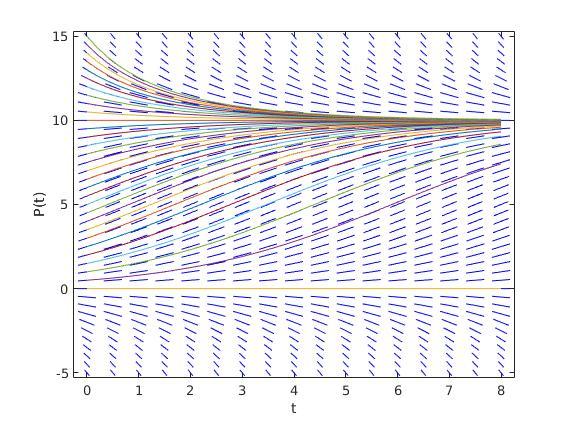
94 Now that we have the solution, let s look at the long term behavior of the solution. The first two terms of the solution will remain finite for all values of t. It is the last term that will determine the behavior of the solution. The exponential will always go to infinity as t goes to infinity, however depending on the sign of the coefficient c ( = y ) is the final behavior. The following analysis gives the long term behavior of the solution for all values of c.

95 Range of c Behavior of solution as c < 0 y c = 0 y finite c > 0 y

96 A graph of several of the solutions is shown below

97 We are now going to start looking at nonlinear first order differential equations. The first type of nonlinear first order differential equations that we will look at is separable differential equations. A separable differential equation is any differential equation that we can write in the following form. or equivalently N(y) dy dx + M(x) = 0 N(y) dy dx = M(x)

98 M(x)dx + N(y)dy = 0 dy dx = M(x) N(y) dy dx = f (x)g(y) Note that in order for a differential equation to be separable all the y s in the differential equation must be multiplied by the derivative and all the x s in the differential equation must be on the other side of the equal sign.

99 Solving a separable differential equation is fairly easy. First of all, we rewrite the differential equation as the following N(y)dy = M(x)dx Then you integrate both sides. N(y)dy = M(x)dx So, after doing the integrations, will have an implicit solution that you can hopefully solve for the explicit solution, y(x). Note that it won t always be possible to solve for an explicit solution.

100 Example 8 Solve the following differential equation and determine the interval of validity for the solution. Solution dy dx = 6y 2 x; y(1) = 1 25 It is clear, that this differential equation is separable. So, let us separate the differential equation and integrate both sides. As with the linear first order officially we will pick up a constant of integration on both sides from the integrals on each side of the equal sign.

101 The two constants can be moved to the same side and absorbed into each other. We will use the convention that puts the single constant on the side with the xs. y 2 dy = 6xdx y 2 dy = 6xdx 1 y = 3x 2 + c Applying initial conditions = 3(1) 2 + c

102 c = 28 Plug this into the general solution and then solve to get an explicit solution. 1 y = 3x 2 28 y(x) = x 2 From the solution we obtained, its natural Domain is < x < 3 ; 3 < x < 3 ; 3 < x <

103 Now, as far as solutions go we ve got the solution. We do need to start worrying about intervals of validity however. The interval must contain the value of the independent variable in the initial condition, x = 1 in this case, and be continuous. However, only one of these will contain the value of x from the initial condition and so we can see that < x < 3 must be the interval of validity for this solution.

104 Here is a graph of the solution.

105 Example 9 Solve the following differential equation and determine the interval of validity for the solution. Solution dy dx = 3x 2 + 4x 4 ; y(1) = 3 2y 4 It is clear, that this differential equation is separable. let us separate the differential equation and integrate both sides. As with the linear first order officially we will pick up a constant of integration on both sides from the integrals on each side of the equal sign.

106 The two can be moved to the same side and absorbed into each other. We will use the convention that puts the single constant on the side with the xs. (2y 4)dy = (3x 2 + 4x 4)dx (2y 4)dy = (3x 2 + 4x 4)dx y 2 4y = x 3 + 2x 2 4x + c Applying initial conditions (3) 2 4(3) = (1) 3 + 2(1) 2 4(1) + c

107 c = 2 Plug this into the general solution and then solve to get an implicit solution. y 2 4y = x 3 + 2x 2 4x 2 We now need to find the explicit solution. This is actually easier than it might look and you already know how to do it. First we need to rewrite the solution a little y 2 4y (x 3 + 2x 2 4x 2) = 0 To solve this all we need to recognize is that this is quadratic in y and so we can use the quadratic formula to solve it.

108 So, upon using the quadratic formula on this we get. y(x) = 4 ± 16 4(1)( (x 3 + 2x 2 4x 2)) 2 y(x) = 4 ± (x 3 + 2x 2 4x 2) 2 y(x) = 2 ± x 3 + 2x 2 4x + 2 Plugging x = 1 into the solution gives. 3 = y(1) = 2 ± = 2 ± 1 = 3, 1

109 In this case it looks like the + is the correct sign for our solution. Note that it is completely possible that the - could be the solution so dont always expect it to be one or the other beforehand. The explicit solution for our differential equation is y(x) = 2 + x 3 + 2x 2 4x + 2 The interval of validity for the solution is given by x : 0 x 3 + 2x 2 4x + 2 x : x

110 Here is graph of the solution.

111 Example 10 Solve the following differential equation and determine the interval of validity for the solution. Solution dy dx = xy 3 ; 1 + x 2 y(0) = 1 First separate and then integrate both sides. y 3 dy = x(1 + x 2 ) 1 2 dx

112 y 3 dy = x(1 + x 2 ) 1 2 dx 1 2y 2 = 1 + x 2 + c Applying initial conditions 1 2 = 1 + c

113 c = 3 2 Plug this into the general solution and then solve to get an implicit solution. 1 2y 2 = 1 + x Now lets solve for y(x). 1 y 2 = x 2 y 2 1 = x 2

114 Solving for y(x) we get. 1 y(x) = ± x 2 Reapplying the initial condition shows us that the minus sign is the correct sign. The explicit solution is then, 1 y(x) = x 2

115 The interval of validity for the solution is given by x : x 2 > 0 x : x 2 < 3 x : 4(1 + x 2 ) < 9 x : (1 + x 2 ) < 9 4

116 x : x 2 < x : 2 < x < 2 And nicely enough, this interval also contains the initial condition x = 0. This interval is therefore our interval of validity.

117 Example 11 Solve the following differential equation and determine the interval of validity for the solution. Solution y = e y (2x 4); y(5) = 0 First separate and then integrate both sides. e y dy = (2x 4)dx

118 e y dy = (2x 4)dx e y = x 2 4x + c Applying initial conditions 1 = e (0) = 5 2 4(5) + c = c

119 c = 4 Plug this into the general solution and then solve to get an implicit solution. e y = x 2 4x 4 Now lets solve for y(x). y = ln(x 2 4x 4)

120 Finding the interval of validity is the last step that we need to take. Recall that we can t plug negative values or zero into a logarithm, so we need to solve the following inequality x : x 2 4x 4 > 0 The two roots of x 2 4x 4 = 0 are: x = 2 ± 2 2 and after a simple analysis we found that, the possible intervals of validity are < x < or < x <

121 From the graph of the quadratic we can see that the second one contains x = 5, the value of the independent variable from the initial condition. Therefore the interval of validity for this solution is < x <

122 Example 12 Solve the following differential equation and determine the interval of validity for the solution. Solution dr dθ = r 2 θ ; r(1) = 2 First separate and then integrate both sides. 1 r 2 dr = 1 θ dθ

123 1 1 r 2 dr = θ dθ 1 r = ln θ + c Applying initial conditions 1 2 = ln 1 + c

124 c = 1 2 Plug this into the general solution and then solve to get an implicit solution. 1 r = ln θ 1 2 Now lets solve for r(θ). 1 r(θ) = 1 2 ln θ

125 Now, there are two problems for our solution here. First we need to avoid θ = 0 because of the natural log. Notice that because of the absolute value on the θ we dont need to worry about θ being negative. We will also need to avoid division by zero. In other words, we need to avoid the following points. θ : 1 2 ln θ = 0 θ : ln θ = 1 2 θ : θ = e 1 2

126 θ : θ = ±e 1 2 So, these three points break the number line up into four portions, each of which could be an interval of validity. θ : < θ < e 1 2 θ : e 1 2 < θ < 0 θ : 0 < θ < e 1 2 θ : e 1 2 < x <

127 The interval that will be the actual interval of validity is the one that contains θ = 1. Therefore, the interval of validity is. θ : 0 < θ < e 1 2

128 Example 13 Solve the following differential equation and determine the interval of validity for the solution. Solution dy dt = ey t sec(y)(1 + t 2 ); y(0) = 0 First separate and then integrate both sides. dy dt = ey e t cos(y) (1 + t2 ) e y cos(y)dy = e t (1 + t 2 )dt

129 e y cos(y)dy = e t (1 + t 2 )dt e y 2 (sin(y) cos(y)) = e t (t 2 + 2t + 1) + c Applying initial conditions 1 2 = 3 + c

130 c = 5 2 Therefore, the implicit solution is: e y 2 (sin(y) cos(y)) = e t (t 2 + 2t + 1) It is not possible to find an explicit solution for this problem and so we will have to leave the solution in its implicit form. Finding intervals of validity from implicit solutions can often be very difficult.

131 We now move into one of the main applications of differential equations. is the process of writing a differential equation to describe a physical situation. Almost all of the differential equations that you will use in your job are there because somebody, at some time, modeled a situation to come up with the differential equation that you are using. This section is designed to introduce you to the process of modeling and show you what is involved in modeling.

132 Mixing Problems In these problems we will start with a substance that is dissolved in a liquid. Liquid will be entering and leaving a holding tank. The liquid entering the tank may or may not contain more of the substance dissolved in it. Liquid leaving the tank will of course contain the substance dissolved in it. If Q(t) gives the amount of the substance dissolved in the liquid in the tank at any time t we want to develop a differential equation that, when solved, will give us an expression for Q(t).

133 Note as well that in many situations we can think of air as a liquid for the purposes of these kinds of discussions and so we dont actually need to have an actual liquid, but could instead use air as the liquid. The main assumption that well be using here is that the concentration of the substance in the liquid is uniform throughout the tank. Clearly this will not be the case, but if we allow the concentration to vary depending on the location in the tank, the problem becomes very difficult.

134 The main equation that well be using to model this situation is : Rate of change of Q(t) = Rate at which Q(t) enters the tank - Rate at which Q(t) exits the tank where, Rate of change of Q(t) = dq(t) dt = Q(t)

135 Rate at which Q(t) enters the tank = (flow rate of liquid entering) x (concentration of substance in liquid entering) Rate at which Q(t) exits the tank = (flow rate of liquid exiting) x (concentration of substance in liquid exiting) Let s take a look at the first problem

136 Example 14 A 1500 gallon tank initially contains 600 gallons of water with 5 lbs of salt dissolved in it. Water enters the tank at a rate of 9 gal/hr and the water entering the tank has a salt concentration of 1 5 (1 + cos(t)) lbs/gal. If a well mixed solution leaves the tank at a rate of 6 gal/hr, how much salt is in the tank when it overflows? We are going to assume that the instant the water enters the tank it somehow instantly disperses evenly throughout the tank to give a uniform concentration of salt in the tank at every point. Again, this will clearly not be the case in reality, but it will allow us to do the problem.

137 Solution Now, to set up the IVP that we will need to solve to get Q(t) we will need the flow rate of the water entering, the concentration of the salt in the water entering, the flow rate of the water leaving (weve got that) and the concentration of the salt in the water exiting (we dont have this ) Since we are assuming a uniform concentration of salt in the tank the concentration at any point in the tank and hence in the water exiting is given by, Concentration = (Amount of salt in the tank at any time t) / ( Volume of water in the tank at any time t)

138 The amount at any time t is easy it s just Q(t). The volume is also pretty easy. We start with 600 gallons and every hour 9 gallons enters and 6 gallons leave. So, if we use t in hours, every hour 3 gallons enters the tank, or at any time t there is t gallons of water in the tank. So, the IVP for this situation is, ( ) ( ) 1 Q(t) Q (t) = (9) (1 + cos(t)) 6 Q(0) = t Q (t) = 9 ( ) Q(t) 5 (1 + cos(t)) 2 Q(0) = t

139 This is a linear differential equation. We will show most of the details, but leave the description of the solution process out. ( Q (t) + 2 Q(t) ) = 9 (1 + cos(t)) t 5 Now find the integrating factor: 2 µ(t) = e 200+t dt = e 2ln(200+t) = e ln(200+t)2 = (200 + t) 2 Now, multiply the rewritten differential equation by the integrating factor. ( ) 2Q(t) (200 + t) 2 Q (t) + (200 + t) 2 = (200 + t) 2 9 (1 + cos(t)) t 5

140 ( (200 + t) 2 Q(t) ) = (200 + t) 2 9 (1 + cos(t)) 5 Integrate both sides and solve for the solution. ((200 + t) 2 Q(t) ) dt = 9 5 (200 + t)2 (1 + cos(t)) dt (200 + t) 2 Q(t) = 9 5 [1 3 (200 + t)3 + (200 + t) 2 sin(t) (200 + t)cos(t) 2sin(t)] + c Q(t) = 9 5 ( 1 3 (200 + t)2 + sin(t) + 2cos(t) t 2sin(t) (200 + t) 2 ) + c (200 + t) 2

141 And applying initial conditions 5 = Q(0) = 9 ( (200) + 2 ) + c 200 (200) 2 c = The solution is then, Q(t) = 9 ( (200 + t)2 + sin(t) + 2cos(t) t 2sin(t) ) (200 + t) (200 + t) 2 Now, the tank will overflow at t = 300hrs. The amount of salt in the tank at that time is. Q(300) = lbs

142

143 Example 15 A 1000 gallon holding tank that catches runoff from some chemical process initially has 800 gallons of water with 2 ounces of pollution dissolved in it. Polluted water flows into the tank at a rate of 3 gal/hr and contains 5 ounces/gal of pollution in it. A well mixed solution leaves the tank at 3 gal/hr as well. When the amount of pollution in the holding tank reaches 500 ounces the inflow of polluted water is cut off and fresh water will enter the tank at a decreased rate of 2 gal/hr while the outflow is increased to 4gal/hr. Determine the amount of pollution in the tank at any time t.

144 Solution The pollution in the tank will increase as time passes. If the amount of pollution ever reaches the maximum allowed there will be a change in the situation. This will necessitate a change in the differential equation describing the process as well. In other words, we ll need two IVP s for this problem. One will describe the initial situation when polluted runoff is entering the tank and one for after the maximum allowed pollution is reached and fresh water is entering the tank. Here are the two IVPs ( for this ) problem. Q 1(t) Q1 (t) = (3)(5) 3 Q(0) = t t m

145 ( ) Q 2(t) Q 2 (t) = (2)(0) (t t m ) Q(t m ) = 500 t m t t e The first one is fairly straight forward and will be valid until the maximum amount of pollution is reached. We ll call that time t m. Also, the volume in the tank remains constant during this time so we dont need to do anything fancy with that this time in the second term as we did in the previous example. We will need a little explanation for the second one. First notice that we do not start over at t = 0. We start this one at t m, the time at which the new process starts. Next, fresh water is flowing into the tank and so the concentration of pollution in the incoming water is zero. This will drop out the first term, and thats okay so don t worry about that.

146 Now, notice that the volume at any time looks a little funny. During this time frame we are losing two gallons of water every hour of the process so we need the 2 in there to account for that. However, we cant just use t as we did in the previous example. When this new process starts up there needs to be 800 gallons of water in the tank and if we just use t there we won t have the required 800 gallons that we need in the equation. So, to make sure that we have the proper volume we need to put in the difference in times. In this way once we are one hour into the new process (i.e t - t m = 1) we will have 798 gallons in the tank as required.

147 Finally, the second process can t continue forever as eventually the tank will empty. This is denoted in the time restrictions as t e. We can also note that t e = t m since the tank will empty 400 hours after this new process starts up. Well, it will end provided something doesn t come along and start changing the situation again. Okay, now that we ve got all the explanations taken care of here s the simplified version of the IVP s that we ll be solving.

148 ( ) Q 1(t) 3Q1 (t) = 15 Q(0) = 2 0 t t m 800 ( ) Q 2(t) Q 2 (t) = 2 Q(t m ) = 500 t m t t e 400 (t t m ) The first IVP is a fairly simple linear differential equation so we will leave the details of the solution to you to check.

149 Q 1 (t) = e 3t 800 Now, we need to find t m. We need to do is determine when the amount of pollution reaches 500. So we need to solve. Q 1 (t) = e 3t 800 = 500 t m = So, the second process will pick up at hours. For completeness sake here is the IVP with this information inserted

150 ( ) Q 2(t) Q 2 (t) = t Q(35.475) = t This differential equation is both linear and separable and I will leave the details to you again to check that we should get. Q 2 (t) = ( t)2 320

151 So, a solution that encompasses the complete running time of the process is Q(t) = { e 3t t ( t) t

152 Here is graph of the solution.

153 Example 16 Escape Velocity The model of constant gravitation only works when were close to the surface of the earth, and the distances we re dealing with are small relative to the radius of the earth. If we start to deal with larger distances, then we must take into account that acceleration from gravity is weaker the farther we are away from the earth. Newton s law of universal gravitation tells us that the force from gravity experienced a distance r from the center of the earth will be: F = GmM r 2

154 where m is the mass of the object, M is the mass of the earth, and G is Newtons gravitational constant G = Nm 2 /kg 2. We can use this relation to calculate an objects escape velocity on the surface of the earth. This is the speed at which an object must be moving away from the earth at the earths surface if it is to break free from the gravitational attraction of the earth and continue to move away forever. Well, we note that if we move away from the earth along a line that goes through the earths center, then Newtons second law tells us: m d 2 r dt 2 = GmM r 2

155 By the chain rule we have dv dt = dv dr dr dr dt, and if we note v = dt then we can transform this relation into mv dv dr = GmM r 2 If we integrate both sides with respect to r we get: 1 2 mv 2 = GmM r + c And applying initial conditions, v(r) = v 0, we obtain: ( 1 v 2 = v GM r 1 ) R

156 If the object is to escape from the graviational action of the earth, then its velocity must always be positive as r. This will be the case if 2GM v 0 R For the earth the escape velocity is v 0 = 11, 180m/s

157 Example 17 Escape Velocity Suppose that you are stranded -your rocket engine has failed- on an asteroid of diameter 3 miles, with density equal to that of the earth with radius 3960 miles. If you have enough spring in your legs to jump 4 feet straight up on earth while wearing your space suit, can you blast off from this asteroid using leg power alone? Solution The escape velocity for the Earth is

158 v E = 2GM E R E Solving for M E in this equation we get: M E = v 2 E R E 2G The density of the earth is its mass divided by its volume M E 4 3 πr3 E = 3v 2 E 8πGR 2 E

159 A similar calculation can be done for the asteroid, and given both the asteroid and the Earth have the same density we get: 3v 2 E 8πGR 2 E = 3v 2 A 8πGR 2 A With a little algebra from this we can deduce the ratio: va 2 ve 2 = R2 A R 2 E So, the escape velocity from the asteroid is

160 ( ) ( ) RA 1.5 v A = v E = 11, 180 = 4.24m/s R E 3960 At the begining of the jump, all the energy is initially kinetic, 1 2 mv 2, and at the top of the jump all that energy is converted into potential energy, mgh. So, the final height is given by the equation: v = 2gh Plugging 4 feet in for h we get: v = 2(9.8)(4ft)(1m/3.28ft) = 4.89m/s > 4.24m/s So, yes, you can get off the asteroid!!!!

161 Example 18 Compound Interest Let S be an initial sum of money. Let r represent an interest rate. We can model the growth of an initial deposit with respect to the interest rate r with differential equations. Let s assume that the initial deposit is compounded continuously. If t represents time, then the rate of change of the initial deposit is ds dt, this quantity is equal to the rate at which interest accrues, which is the interest rate r times the current value of the investment S(t). Thus, the model is given by ds dt = rs(t)

162 Suppose that we also know the value of the investment at some particular time, say, S(0) = S 0 Integrating this separable IVP ds dt = rs(t) 1 ds = rdt S 1 S ds = ln S = rt + K rdt

163 S(t) = ce rt and using the initial condition that S(0) = S 0, we have that the constant of integration is c = S 0. Therefore the solution to this initial value problem is: S(t) = S 0 e rt

164 Example 19 Compound Interest Let S be an initial sum of money. Let r represent an interest rate. Assume that the initial deposit is compounded continuously. Let suppose that there may be deposits or withdrawals in addition to the accrual of interest, dividends, or capital gains and the deposits or withdrawals take place at a constant rate k. So the IVP is ds dt = rs(t) + k S(0) = S 0 ( k > 0 for deposits and k < 0 for withdrawals)

165 The above differential equation is a linear one, with integrating factor e rt, so its general solution is: S(t) = ce rt k r and using the initial condition that S(0) = S 0, we have that the constant of integration is c = S 0 + k r. Therefore the solution to this initial value problem is: S(t) = S 0 e rt + k ( e rt 1 ) r

166 Example 20 Newton s Law of Cooling Newton s Law of Cooling states that the temperature of a body changes at a rate proportional to the difference in temperature between its own temperature and the temperature of its surroundings. We can therefore write dt dt = k (T T s)

167 where, T = Temperature of the body at any time t T s = Temperature of the surroundings (also called ambient temperature) T 0 = Initial temperature of the body k = constant of proportionality Integrating this separable differential equation dt dt = k (T T s)

168 1 dt = kdt T T s 1 dt = T T s ln T T s = kt + C T T s = e kt+c kdt

169 T = T s + ce kt ; T > T s (why?) Applying initial conditions T (0) = T 0 c = T 0 T s Thus, the solution is T = T s + (T 0 T s )e kt

170 Theorem 1 (Existence and Uniqueness). Suppose p(t) and g(t) are continuous real-valued functions on an interval (α, β) that contains the point t 0. Then, for any choice of (initial value) y 0, there exists a unique solution y(t) on the whole interval (α, β) to the linear differential equation dy(t) dt for all t (α, β) and y(t 0 ) = yo. + p(t)y(t) = g(t)

171 Theorem 2 (Existence and Uniqueness). Suppose that both f (t, y) and f (t, y) are continuous functions y defined on a region R as R = {(t, y) : t 0 δ < t < t 0 + δ; y 0 ɛ < y < y 0 + ɛ} containing the point (t 0, y 0 ). Then there exists a number δ 1 (possibly smaller than δ) so that a solution y = f (t) to y = f (t, y) y(t 0 ) = y 0 is the unique solution for t 0 δ 1 < t < t 0 + δ 1

172 Example 21 Consider the ODE y = t y + 1; y(1) = 2 In this case, both the function f (t, y) = ty + 1 and its partial derivative f (t, y) = 1 are defined and continuous at all points y (x, y). The Theorem 2 guarantees that a solution to the ODE exists in some open interval centered at 1, and that this solution is unique in some (possibly smaller) interval centered at 1.

173 In fact, an explicit solution to this equation is y(t) = t + e 1t This solution exists (and is the unique solution to the equation) for all real numbers t. In other words, in this example we may choose the numbers δ and δ 1 as large as we please. Example 22 Consider the ODE y = 1 + y 2 ; y(0) = 0

174 In this case, both the function f (t, y) = 1 + y 2 and its partial derivative f (t, y) = 2y are defined and continuous at all points y (t, y). The Theorem 2 guarantees that a solution to the ODE exists in some open interval centered at 0, and that this solution is unique in some (possibly smaller) interval centered at 1. By separating variables and integrating, we derive a solution to this equation of the form y(t) = tan(t)

175 As an abstract function of t, this is defined for all t..., 3π/2, π/2, π/2, 3π/2,... However, in order for this function to be considered as a solution to this ODE, we must restrict the domain. Specifically, the function y(t) = tan(t); π/2 < x < π/2 is a solution to the above ODE. In this example we must choose δ 1 = π/2, although the initial value δ, may be chosen as large as we please.

176 One particular case of a separable equation is the so called Autonomous Equation, which is an equation of the form dy dt = f (y) That is, the right hand side only depends on y and therefore the directional field can be found only analyzing horizontal lines. We will use some concrete examples to see how we can use a qualitative analysis to determine the behavior of the function.

177 Population If P(t) represents a population in a given region at any time t the basic equation that we will use is : Rate of change of P(t) = Rate at which P(t) enters the region - Rate at which P(t) exits the region Here the rate of change of P(t) is still the derivative. For population problems all the ways for a population to enter the region are included in the entering rate. Birth rate and migration into the region are examples of terms that would go into the rate at which the population enters the region.

178 Likewise, all the ways for a population to leave an area will be included in the exiting rate. Therefore things like death rate, migration out and predation are examples of terms that would go into the rate at which the population exits the area. Example 23 A population of insects in a region will grow at a rate that is proportional to their current population. In the absence of any outside factors the population will triple in two weeks time. On any given day there is a net migration into the area of 15 insects and 16 are eaten by the local bird population and 7 die of natural causes. If there are initially 100 insects in the area will the population survive? If not, when do they die out?

179 Solution Let s start out by looking at the birth rate. We are told that the insects will be born at a rate that is proportional to the current population. This means that the birth rate can be written as rp(t) where r is a positive constant that will need to be determined. Now, let s take everything into account and get the IVP for this problem. P (t) = (rp + 15) (16 + 7) P(0) = 100 P (t) = rp 8 P(0) = 100

180 Note that we don t make use of the fact that the population will triple in two weeks time in the absence of outside factors here. In the absence of outside factors means that the only thing that we can consider is birth rate. Nothing else can enter into the picture and clearly we have other influences in the differential equation. So, just how does this tripling come into play? We will use the fact that the population triples in two week time to help us find r. In the absence of outside factors the differential equation would become. P (t) = rp P(0) = 100 P(14) = 300

181 This differential equation is separable and linear and is a simple differential equation to solve. The general solution is : P(t) = ce rt Applying the initial condition gives c = 100. Now apply the second condition. 300 = P(14) = 100e 14r And solving for r, we have r = ln3 14

182 Now, that we have r we can go back and solve the original differential equation. ( ) ln3 P (t) P = 8 P(0) = This is a simple linear differential equation, with integrating fractor given by: µ(t) = e ln3 14 dt = e ln3 14 t And the solution is ( Pe ln3 t) 14 dt = 8 e ln3 14 t dt

183 P(t) = 112 ln3 + ce ln3 14 t And applying the initial condition, we get P(t) = 112 ln3 + ( ) 3 e ln3 14 t = 112 ln3 (1.947) e 14 t ln3 Now, the exponential has a positive exponent and so will go to plus infinity as t increases. Its coefficient, however, is negative and so the whole population will go negative eventually. Since the population cannot be negative, there is a time such that all of them die out

184 112 ln3 t = 50.4 (1.9468) e ln3 14 t = 0 days Thus, the insects will survive for around 7 weeks.

185 Example 24 Logistic Growth Previously we have modeled a population based on the assumption that the growth rate would be a constant A much more realistic model of a population growth is given by the logistic growth equation. Here is the logistic growth equation. ( P = r 1 P ) P K In the logistic growth equation r is the intrinsic growth rate. It is the growth rate that will occur in the absence of any limiting factors. K is called either the saturation level or the carrying capacity.

186 Now, we claimed that this was a more realistic model for a population. Lets see if that in fact is correct. To allow us to sketch a direction field let s pick a couple of numbers for r and K. We will use r = 1/2 and K = 10. For these values the logistics equation is. P = 1 2 ( 1 P 10 ) P First notice that the derivative will be zero at P = 0 and P = 10. Also notice that these are in fact solutions to the differential equation. These two values are called equilibrium solutions since they are constant solutions to the differential equation. Here is the direction field and some solutions sketched in as well.

187