5.8 Laminar Boundary Layers

Size: px

Start display at page:

Download "5.8 Laminar Boundary Layers"

Ezra Anthony
5 years ago
Views:

1 2.2 Marine Hydrodynamics, Fall 218 ecture 19 Copyright c 218 MIT - Department of Mechanical Engineering, All rights reserved Marine Hydrodynamics ecture aminar Boundary ayers δ y U potential flow u, v viscous flow x Uo Assumptions 2D flow: w, z and u x, y), v x, y), p x, y), U x, y). Steady flow: t. For δ <<, use local body) coordinates x, y, with x tangential to the body and y normal to the body. u tangential and v normal to the body, viscous flow velocities used inside the boundary layer). U, V potential flow velocities used outside the boundary layer). 1

2 5.8.2 Governing Equations Continuity Navier-Stokes: u x + v y = 1) u u x + v u y = 1 ρ u v x + v v y = 1 ρ ) p 2 x + ν u x + 2 u 2 y 2 ) p 2 y + ν v x + 2 v 2 y 2 2) 3) Boundary Conditions KBC Inside the boundary layer: No-slip ux, y = ) = No-flux vx, y = ) = Outside the boundary layer the velocity has to match the P-Flow solution. et y y/δ, Y Y/, and x x/, X X/. Outside the boundary layer y but Y. We can write for the tangential and normal velocities ux, y ) = UX, Y ) and vx, y ) = V X, Y ) = No-flux P-Flow In short: ux, y ) = Ux, ) vx, y ) = DBC As y, the pressure has to match the P-Flow solution. The x-momentum equation at y = gives U U x + V U y = 1 dp ρ dx + ν 2 U y 2 dp dx = ρu U x 2

3 5.8.4 Boundary ayer Approximation Assume that R e >> 1, then u, v) is confined to a thin layer of thickness δ x) <<. For flows within this boundary layer, the appropriate order-of-magnitude scaling / normalization is: Variable Scale Normalization u U u = Uu x x = x y δ y = δy v V =? v = Vv Non-dimensionalize the continuity, Equation 1), to relate V to U U ) u + V x δ ) ) v δ = = V = O y U Non-dimensionalize the x-momentum, Equation 2), to compare δ with U 2 u u ) + UV v u ) = 1 p x }{{} δ y ρ x + νu ) δ 2 2 ) u 2 u + δ 2 2 x }{{ 2 y } 2 OU 2 /) ignore The inertial effects are of comparable magnitude to the viscous effects when: U 2 νu δ = δ ν 2 U = 1 << 1 Re The pressure gradient p x must be of comparable magnitude to the inertial effects p x = O ρ U ) 2 3

4 Non-dimensionalize the y-momentum, Equation 3), to compare p y p 2 v UV }{{} O U2 δ ) u v ) + V2 x }{{} δ O U2 The pressure gradient p y δ ) Comparing the magnitude of p x Note: v v ) = 1 y ρ y + νv }{{} 2 O U2 δ 3 3 ) x 2 ) + νv to p x δ 2 }{{} O U2 δ ) 2 v y 2 must be of comparable magnitude to the inertial effects p ρ y = O U ) 2 δ to p y we observe p = O ρ U ) 2 δ while p ρ y x = O U ) 2 = p << p = p y x y = p = px) - From continuity it was shown that V/U Oδ/) v << u, inside the boundary layer. - It was shown that p =, p = px) inside the boundary layer. This means that y the pressure across the boundary layer is constant and equal to the pressure outside the boundary layer imposed by the external P-Flow. ) 4

5 5.8.5 Summary of Dimensional BVP Governing equations for 2D, steady, laminar boundary layer Boundary Conditions KBC Continuity : u x + v y = x-momentum : u u x + v u y = y - momentum : p y = At y= : ux, ) = vx, ) = 1 dp ρ dx }{{} UdU/dx, y= At y/δ : ux, y/δ ) = Ux, ) vx, y/δ ) = +ν 2 u y 2 DBC dp dx U = ρu x or IN the b.l. px) = C 1 2 ρu 2 x, ) }{{} Bernoulli for the P-Flow at y = Definitions Displacement thickness δ 1 u ) dy U Momentum thickness θ u U 1 u ) dy U 5

6 Physical Meaning of δ and θ Assume a 2D steady flow over a flat plate. Recall for steady flow over flat plate dp dx = and pressure p = const. Choose a control volume [, x] [, y/δ ]) as shown in the figure below. y /δ Uo Q 4 CV Uo U o P - Flow 3 1 Boundary ayer x CV for steady flow over a flat plate. 2 uy) Control Volume book-keeping Surface ˆn v v ˆn v v ˆn) pˆn 1 î U o î U o Uo 2î pî 2 ĵ pĵ 3 î ux, y)î + vx, y)ĵ ux, y) u 2 x, y)î + ux, y)vx, y)ĵ pî 4 ĵ U o î + vx, y)ĵ vx, y) vx, y)u o î + v 2 x, y)ĵ pĵ 6

7 Conservation of mass, for steady CV v ˆndS = U o dy Q = U o dy udy = where ) are the dummy variables. Conservation of momentum in x, for steady CV ρ u v ˆn)dS = F x 1234 [ ρ Uo 2 dy + ρ ρ ρ ρu 2 o U 2 o dy + ρ U 2 o dy + ρ u 2 x, y )dy + x ux, y )dy + vx, y)dx = }{{} ) U o u)dy = U o 1 uuo dy Q = U δ }{{} δ x vx, y)u o dx ] = Q pdy x u 2 x, y )dy + ρu o vx, y)dx = F x,friction }{{} Q u 2 x, y )dy + ρu o U o u)dy = F x,friction ) Uo 2 + u 2 + Uo 2 U o u dy = F x,friction u 2 U 2 o u U o )dy = F x,friction ) Fx,friction = ρuo 2 u 1 uuo dy F x,friction = ρuo 2 θ U } o {{} θ pdy + F x,friction 7

8 5.9 Steady Flow over a Flat Plate: Blasius aminar Boundary ayer y U o x Steady flow over a flat plate: BB Derivation of BB Assumptions Steady, 2D flow. Flow over flat plate U = U, V =, dp dx = B governing equations Boundary conditions u x + v y = u u x + v u y = ν 2 u y 2 u = v = on y = v V =, u U o outside the B, i.e., y δ >> 1 ) Solution Mathematical solution in terms of similarity parameters. u U and η y Uo Similarity solution must have the form νx y x = u x, y) = F η) U } o {{} self similar solution 8 η νx y = η Rx U o

9 We can obtain a PDE for F by substituting into the governing equations. The PDE has no-known analytical solution. However, Blasius provided a numerical solution. Once again, once the velocity profile is evaluated we know everything about the flow Summary of BB Properties: δ, δ.99, δ, θ, τ o, D, C f u x, y) = F U o }{{} η) ; evaluated numerically η = y Uo νx ; νx y η ; U o y x = η Rx }{{} local R# νx δ U o δ.99 = 4.9 νx U o, i.e., η.99 = 4.9 δ = 1.72 νx U o, i.e., η = 1.72 δ x, δ 1/ Uo δ ν x U o x = 1 Rx θ νx =.664 U o ) 1/2 τ o τ w =.332ρU 2 Uo x o ν τ o 1 x =.332 ρu 2 o ) R 1/2 x }{{} local R# τ o U 3/2 o 9

10 Total drag on plate x B D = B }{{} width ) 1/2 τ o dx =.664 ) ρuo 2 Uo B) ν }{{} Re 1/2 D, D U 3/2 Friction drag) coefficient: D C f = 1 ρu 2 2 o ) B) = C f 1, C f 1 Re U.8 C f Blasius aminar Boundary ayer C f Re Turbulent Boundary ayer Turbulent Boundary ayer C f for flat plate JNN 2.3) Rex ~ 3 1 Transition at Reδ ~ 6 5 Re Skin friction coefficient as a function of R e. A look ahead: Turbulent Boundary ayers Observe form the previous figure that the function C f, laminar R e ) for a laminar boundary layer is different from the function C f, turbulent R e ) for a turbulent boundary layer for flow over a flat plate. Turbulent boundary layers will be discussed in proceeding ecture. 1

11 5.1 aminar Boundary ayers for Flow Over a Body of General Geometry The velocity profile given in BB is the exact velocity profile for a steady, laminar flow over a flat plate. What is the velocity profile for a flow over any arbitrary body? In general it is dp/dx and the boundary layer governing equations cannot be easily solved as was the case for the BB. In this paragraph we will describe a typical approximative procedure used to solve the problem of flow over a body of general geometry. 1. Solve P-Flow outside B B 2. Solve boundary layer equations with P term) get δ x) 3. From B + δ B 4. Repeat steps 1) to 3) until no change U y B x P U const. von Karman s zeroth moment integral equation τ ρ = d U 2 x)θx) ) + δ x)ux) du dx dx 4) Approximate solution method due to Pohlhausen for general geometry dp/dx ) using von Karman s momentum integrals. The basic idea is the following: we assume an approximate velocity profile e.g. linear, 4 th order polynomial,...) in terms of an unknown parameter δx). From the velocity profile we can immediately calculate δ, θ and τ o as functions of δx) and the P-Flow velocity Ux). Independently from the boundary layer approximation, we obtain the P-Flow solution outside the boundary layer Ux), du dx. Upon substitution of δ, θ, τ o, Ux), du in von Karman s moment integral equations) dx we form an ODE for δ in terms of x. 11

12 Example for a 4 th order polynomial Pohlhausen velocity profile Pohlhausen profiles - a family of profiles as a function of a single parameter Λx) shape function factor). Assume an approximate velocity profile, say a 4 th order polynomial: u x, y) U x, ) = a x) y y ) 2 y ) 3 y ) 4 δ + b x) + c x) + d x) 5) δ δ δ There can be no constant term in 5) for the no-slip BC to be satisfied y =, i.e, ux, ) =. We use three BC s at y = δ u U = 1, u y =, 2 u =, at y = δ 6) y2 From 6) in 5), we re-write the coefficients ax), bx), cx) and dx) in terms of Λx) a = 2 + Λ/6, b = Λ/2, c = 2 + Λ/2, d = 1 Λ/6 To specify the approximate velocity profile ux,y) in terms of a single unknown Ux,) parameter δ we use the x-momentum equation at y =, where u = v = u u x + v u y = U U + ν 2 u x }{{} y 2 b = 1 ) du δ 2 Λx) = du δ 2 x) }{{ y= 2 dx ν dx ν } 1 dp ρ dx ν 2bU δ 2 Observe: Λ du { Λ > : favorable pressure gradient dx Λ < : adverse pressure gradient Putting everything together: u x, y) U x, ) = 2 y ) y ) 3 y ) δ δ δ + du [ δ 2 1 y ) 1y dx ν 6 δ 2 δ ) y δ ) ] y ) 4 δ 12

13 Once the approximate velocity profile ux,y) is given in terms of a single unknown Ux,) parameter δx), then δ, θ and τ o are evaluated Notes: δ = θ = δ 1 u ) 3 dy = δ U 1 1 du 12 dx δ 2 ) ) ν u 1 u ) 37 dy = δ U U du 945 dx τ o = µ u y = µu y= δ du 6 dx δ 2 ) ) ν δ 2 ) 1 du ν 972 dx ) δ 2 ) 2 ν - Incipient flow τ o = ) for Λ = 12. However, recall that once the flow is separated the boundary layer theory is no longer valid. - For du = Λ = Pohlhausen profile differs from Blasius B only by a dx few percent. After we solve the P-Flow and determine Ux), du we substitute everything into dx von Karman s momentum integral equation 4) to obtain dδ dx = 1 du U dx gδ) + d2 U/dx 2 du/dx hδ) where g, h are known rational polynomial functions of δ. This is an ODE for δ = δx) where U, du, d2 U are specified from the P-Flow dx dx 2 solution. General procedure: 1. Make a reasonable approximation in the form of 5), 2. Apply sufficient BC s at y = δ, and the x-momentum at y = to reduce 5) as a function a single unknown δ, 3. Determine Ux) from P-Flow, and 4. Finally substitute into Von Karman s equation to form an ODE for δx). Solve either analytically or numerically to determine the boundary layer growth as a function of x. 13

14 Appendix A 14

15 15

16 16

17 17

18 18

19 19

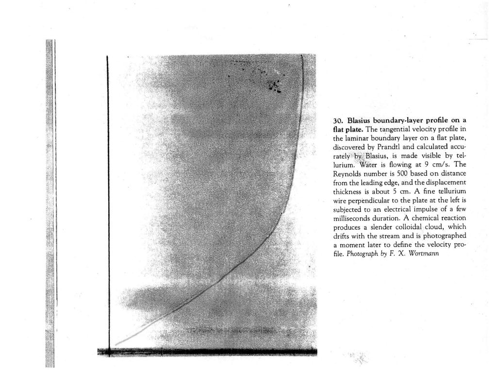
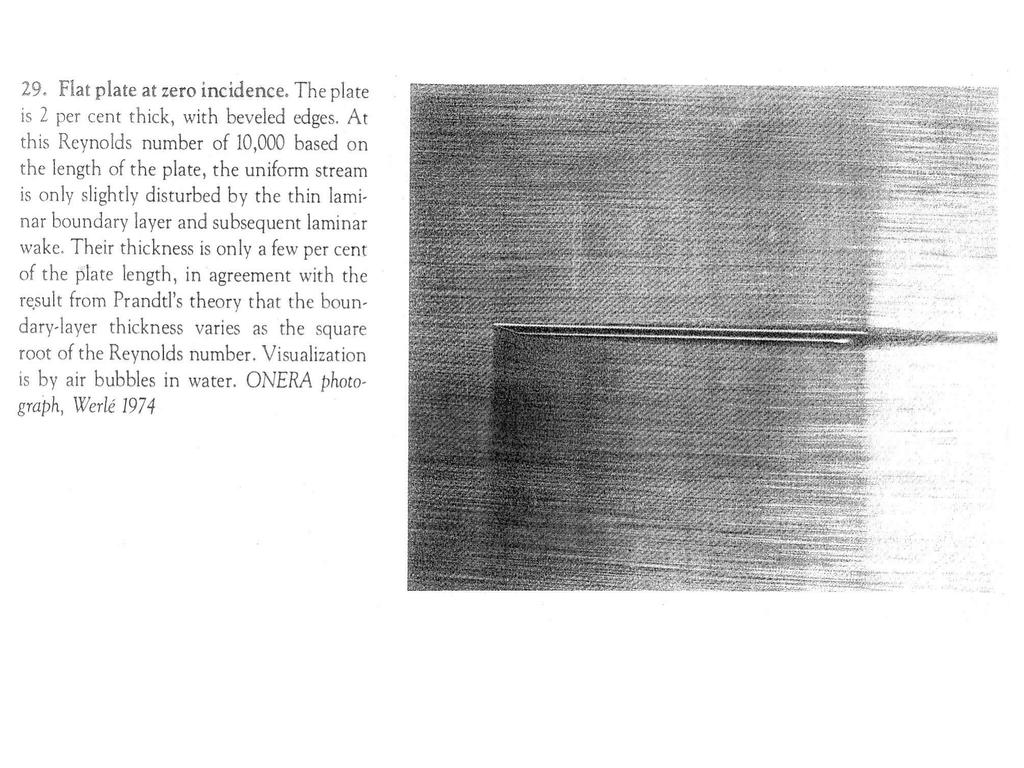
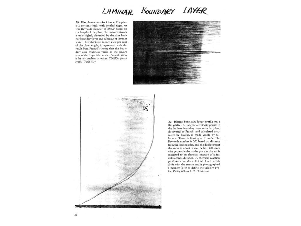
9. Boundary layers. Flow around an arbitrarily-shaped bluff body. Inner flow (strong viscous effects produce vorticity) BL separates

9. Boundary layers. Flow around an arbitrarily-shaped bluff body. Inner flow (strong viscous effects produce vorticity) BL separates 9. Boundary layers Flow around an arbitrarily-shaped bluff body Inner flow (strong viscous effects produce vorticity) BL separates Wake region (vorticity, small viscosity) Boundary layer (BL) Outer flow