Computational Explorations in Cognitive Neuroscience Chapter 5: Error-Driven Task Learning

Transcription

1 Computational Explorations in Cognitive Neuroscience Chapter 5: Error-Driven Task Learning 1

2 5.1 Overview In the previous chapter, the goal of learning was to represent the statistical structure of the input space (environment). A different learning goal is to represent the mapping of an input pattern to an output pattern. This is similar to stimulus-response learning. It is also called task learning. Unfortunately, the CPCA Hebbian learning rule does not perform well for this type of learning. 2

3 However, there is an alternative rule that can handle it, called the delta rule. This rule involves supervised learning because it supervises the learning to adjust weights according to discrepancies (errors) between the actual output and a target output. It is also called error-driven because it uses these errors in task performance to adjust weights. When the delta rule is generalized to multiple layers, it is called backpropagation because errors are propagated backward from higher layers to lower layers, transforming weights in multiple layers in a consistent fashion that brings the network closer to solving the task. A backpropagation algorithm that uses bi-directional activation propagation to communicate error signals is called generalized recirculation (GeneRec). 3

4 5.2 Exploration of Hebbian Task Learning There are 2 simulations in this section, one involving an easy input-output mapping, and one involving a hard one. The network has 4 input units and 2 output units. The task is defined in terms of learning the relationship between activation patterns over the input layer and the target values of the output units. This network is called a pattern associator because it tries to associate input and output patterns. A training epoch consists of presenting each of the 4 events. Training input-output relations involves clamping the input and output units to their values corresponding to the events in the environment. At the end of each epoch, a testing phase is run. In the testing phase, all 4 events are presented to the network, without the output units being clamped, and the output activations are computed based on the inputs and the weights that were trained. 4

5 Network performance is tested by computing the summed squared error (SSE), which is based on the difference between the actual output activation (o k ) and the target value (t k ). The SSE is defined as: ( ) 2 k k (5.1) k SSE = t o where the summation is over all k output units. The difference in this equation is the basis for error-driven learning. It requires a target value which has to be provided by the outside teacher or supervisor. The difference is squared to remove the sign, since we aren t concerned with whether o k is above or below t k, just how different they are. SSE goes to zero when all the outputs exactly match their targets for all events in the environment (also called the training set). If the actual output activation matches the target value, then the error is eliminated, SSE is zero, and the task has been learned. 5

6 The first simulation is a pattern associator task that categorizes two inputs as left and two as right. Pre-training weights to each receiving unit are randomly distributed across the input units: 6

7 There are 4 training events that associate the left 2 input units with the left receiving unit and the right 2 input units with the right receiving unit. 7

8 The network is trained by clamping both the input and output units to their corresponding values from the events in the environment, and CPCA Hebbian learning is performed on the resulting activations. 8

9 The network is able to easily learn this task: Test grid log Receiving weights 9

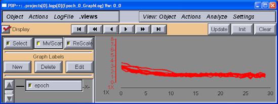
10 The SSE quickly goes to 0 after a couple of epochs: Training graph log 10

11 Question 5.1: For the easy environment, the Hebbian learning rule works well because the input-output mapping is based on the correlation structure of the input space. This means that the task can be solved simply by learning the features of the environment, something we have already seen that Hebbian learning is good at. 11

12 For the hard environment, there is nothing about the correlation structure of the input space that can be used to successfully learn the correct input-output mapping. 12

13 Question 5.2: (a) For the hard environment, the network is never able to solve the task, and SSE never goes to zero. (b) The sums of the thresholded SSE measure (across all events) for several runs: 2.05, 1.65, 2.05, 2.25,

14 5.3 Using Error to Learn: The Delta Rule We want to derive a learning rule that will make direct use of errors in task performance to adjust weights. For any given output unit and input event, we want to change the weight in such a way that the error will be reduced. The error is given by the SSE: ( ) 2 k k SSE = t o There is now a second summation over all events, indexed by t. t Our goal is to find a learning rule that will determine how a weight should be changed so as to minimize SSE. We would like this rule to change the weight in a way that reduces, and eventually minimizes, the error. A way to find this rule is based on the local slope of the relation between error and weight. To reduce the error means that we must change the weight in the direction opposite to the sign of the slope, with a magnitude equal to the absolute value of this local slope. k 14

15 Criteria for a error-driven learning rule 1) When the slope is large and positive, the rule should decrease w ik by a relatively large amount. 2) When the slope is large and negative, the rule should increase it by a relatively large amount. 3) As the slope gets smaller as it approaches zero, the rule should change w ik by a correspondingly small amount. 15

16 To satisfy these criteria: Δw ik b g ΔSSE Δ tk o 2 k = = Δw Δw ik ik For an arbitrarily small weight change, this is expressed as a derivative: Δw ik SSE = w ik b g 2 k tk o = w ik Using the chain rule: Δw ik SSE = w ik b g 2 k tk o = o k o w k ik Using the chain rule again: Δw ik SSE = w ik b b tk ok = t o k g2 g k b t k o o k k g o w k ik 16

17 Now, solving for the first expression on the RHS: Δw ik We have now derived: SSE = w ik b ga f b g k ik ok = 2 tk ok 1 = 2 tk o w o w k ik b t o g 2 k k = SSE = 2 b tk o g k o o k k (5.5*) o w k We must next solve for. ik We can do this by using a simple linear activation function for the output unit: where s i is the activity of a sending unit. o = s w (5.6) k i ik i 17

18 The derivative of this output function with respect to the weight is: o s w = = s k i ik i wik w (5.7) ik Putting 5.5* and 5.7 together, we get: ( t o ) k k Δ w = = 2( t o ) s w ik k k i ik Since the 2 is an arbitrary constant, we can substitute a learning rate parameter (ε) as before. Therefore we get the following learning rule: which is called the delta rule. ( ) Δ wik = ε tk ok si (5.9) 2 18

19 How will the delta learning rule adjust the weights to reduce the error? A weight will change as a function of: (1) the local error for the individual output unit (i.e. t k - o k ), increasing the weight when the actual output activation is less than the target value and decreasing it when it is greater; and (2) the activation of the sending unit (i.e. s i ). 19

20 Credit (Blame) Assignment Those sending units that are most active when a big error is made will get most of the blame for this error. Assigning them blame will reduce their ability to cause this error again in the future. How is blame assigned? Example 1: if an output unit is active when it shouldn t be, then (t k - o k ) is negative and the weights will be decreased to the output unit from those input units that are active (in proportion to their activity levels). This will reduce future errors because the output unit will be less active to the same input pattern. Example 2: if an output unit is not active when it should be, then (t k - o k ) is positive and the weights will be increased to the output unit from those input units that are active (in proportion to their activity levels). This will reduce future errors because the output unit will be more active to the same input pattern. 20

21 The process of adjusting weights in proportion to the sending unit activations is called credit (blame) assignment. Credit assignment can be seen within the framework of constraint satisfaction, i.e. errordriven learning is the result of multiple credit satisfaction. This type of constraint satisfaction, though, is fundamentally different than in Hebbian learning. The representations do not reflect the strongest correlations of the input space. Rather, they reflect the solutions that best satisfy the desired input-output mapping. 21

22 5.3.2 Learning Bias Weights The bias weight (β i ) can be used with task learning to provide an additional input to a receiving unit. Furthermore, it can be trained by considering it to come from an additional input unit that is always on (i.e. s i = 1). That is: ( t o ) Δ βk = ε k k (5.10) The bias weight will provide additional correction for the receiving unit so that its error is decreased. Any relatively constant error caused by the unit being too active or too inactive will be corrected. 22

23 5.4 Error Functions, Weight Bounding, and Activation Phases There are 3 problems with using the delta rule: 1. It is based on a linear activation function, but our network units use the point-neuron activation function described in Chapter 2 (Box 2.2). 2. It allows weights to switch sign and take on any value, violating the biological intuition that weights should be bounded. 3. It uses target output values, a device that violates intuitions about neurobiological reality. (i.e. what sets such targets in the brain?) 23

24 5.4.1 Cross Entropy Error To address the first problem with the delta rule requires that we use a different error function; one which takes into account the saturation property of the sigmoid activation function. The new error function is called cross entropy. In general, entropy is defined as: = b g i i b g i HX ( ) px log px Where X is a random variable and P(X) is a probability density function on X. Cross entropy is similarly defined as: c h i log( i ) ( ) m( x ) p x i where p and m are two probability density functions on X. 24

25 Here we use the cross entropy as an error function. We treat t k and o k as probability functions, and sum together two cross entropy terms: ( 1 ) log( 1 ) CE = tk log ok + tk ok (5.11) t k We summate these terms over both t (events) and k (output units). Note that, since the target activation t k is either 0 or 1, only one of these cross entropy terms is in effect at any given time. Hence: 1. When t k is 1, the 1 st term on the RHS is in effect and the 2 nd term is 0. In this case, the error depends on -log(o k ), decreasing (becoming more negative) as o k increases. 2. When t k is 0, the 1 st term is 0 and the 2 nd term is in effect. Then, the error depends on -log(1- o k ), increasing (becoming less negative) as o k increases. In Figure 5.5 the target value is 1. If the activity level (o k ) is at the target value, its maximum value, then CE is zero. CE increases as o k decreases. As o k nears 0, CE grows exponentially large. 25

26 To derive the weight update rule for the CE error function, we can determine how the error changes for an arbitrarily small weight change. Thus, we again take the derivative of the error with respect to the weight (and use the chain rule): CE CE ok ηk = w o η w (5.14) ik k k ik where the net input to the output unit is: η = sw (5.12) k i ik i and the activity level of the output unit is: o k 1 = + (5.13) e η 1 k 26

27 Solving for the first term on the RHS of Equation 5.14: ( 1 o ) ( t log o ( 1 t ) log ( 1 o )) ( t log o ) ( 1 t ) log( 1 o ) + = = o o o o CE k k k k k k k k k k k k ( ) ( ) ( ) ( ) ( ) ( ) t k t t o t o t o k = = + = o 1 o o 1 o o 1 o o 1 o tk ok = o k k k k k k k k k k k k k k k k (5.15) For the 2 nd term, we accept the derivation given on p. 155: o ( 1 o ) = o k k k η (5.16) k For the 3 rd term, the derivative of the net input is the same as the derivative of the output of the simple linear activation derived before: η = s k i w (5.17) ik 27

28 Putting these 3 together, we get: CE w ik ( ) = tk ok si (5.18) which (taking the negative) gives the same delta rule as Eq. 5.9: ε ( ) Δ w = t o s. ik k k i We thus see that by using the CE error function instead of the SSE error function, the activation function can be sigmoidal instead of linear, and the delta rule still applies. 28

29 5.4.2 Soft Weight Bounding Here we deal with the second problem with the delta rule. As discussed in Section 4.5.3, CPCA has natural soft weight bounding, meaning that the weights saturate at the upper and lower bounds. As was noted, soft weight bounding is biologically consistent in that LTP/LTD has the same property. The basic delta rule lacks this property. However, it can be imposed by the following transformation: b g (5.19) Δw = Δ 1 w + Δ w ik ik + ik ik ik where: w ik is the weight value, Δ ik is the weight change computed by the error-driven algorithm, [x] + means return x if x > 0 and 0 otherwise, and [x] - means return x if x < 0 and 0 otherwise. This transformation causes the weight change to decrease more and more as it gets closer to 1 or 0; thus the weight values approach their 0 and 1 limits exponentially slowly. 29

30 5.4.3 Activation Phases in Learning We now turn to the third problem with the delta rule the target signal. A biologically plausible interpretation of the target value (t k ) is that it is an activation state that corresponds to an observed outcome of an event in the world. If so, the activation state of the output unit (o k ) may be interpreted as an expectation of the outcome. In the previous simulation, we trained the network with the Hebbian update rule during the training phase and tested the network performance during the testing phase. In the next simulation, we will train the network with the delta update rule. There will still be two phases, but we will give them different meanings, and their temporal ordering will be different. The two phases for every input event: 1) The first (minus) phase does not have the output unit values clamped. The output units are activated according to the inputs and the weights. This gives the expectation, now called o k -. 2) The second (plus) phase has the output unit values clamped. This gives the outcome, now called o k +. 30

31 After we run the minus phase followed by the plus phase, we then use the difference between the two outputs to adjust the weights: εc h (5.20) + Δw = o o s ik k k i Note that the expression for the delta rule is modified to reflect the minus and plus phase activations. This form of the delta rule will only be of value if it allows us to implement the rule in a more biologically realistic way. We will see that this is true further down when we encounter the GeneRec algorithm. 31

32 5.5 Exploration of Delta Rule Task Learning The network and environment are the same as in the previous simulations, but the delta rule is now used. With the step_level parameter set to STEP_SETTLE, you can see each phase of processing. The first time an input pattern is presented, the actual activation produced by the network weights in response to the input pattern is seen. This is the minus phase. The second time it is presented, the clamped target activation is seen. This is the plus phase. The weights are updated by the delta rule after the plus phase. The network is able to learn both the easy and hard environments using the delta rule. 32

33 Easy: Weights before training Weights after training 33

34 Activation at start Activation at end Error log 34

35 Hard: Activation at start Activation at end Error log 35

36 Impossible: 36

37 Question 5.3: (a) Using the delta rule, the weights always tend to be evenly distributed across the input units for each output unit. The 1 st input unit tends to be most often weighted to the left output unit, whereas the 2 nd input unit tends to be most often weighted to the right. The bias weights tend to be almost always weighted toward the right output unit. Using the Hebbian rule, the 1 st and 4 th input units do not contribute very much to the left output unit, with all the emphasis put on the middle two input units. This is because the two input patterns that are targeted to activate the left output unit share the middle two input units as a feature. By contrast, the right output unit has little weight from the 1 st input unit, greatest weight from the 2 nd input unit, and minor weights from the 3 rd and 4 th input units. This is because the 1 st input unit does not contribute to the right output unit, the 2 nd input unit is common to both its input patterns, and the 3 rd and 4 th input units each partially contribute. (b) The Hebbian rule is unsuccessful because it learns that the middle two input units are the feature of the left output unit, but this feature also codes for the right output unit in event_3. Also, it learns that the 2 nd input unit is a feature of the right output unit, but this feature also codes for the left output unit in event_0 and event_1. 37

38 The delta rule is successful because it learns that the 1 st input unit being on predicts the left output unit being the target. It also learns that when the 1 st input unit is off, the other 3 being on also predicts the left output unit being the target, and a combination of 2 predicts the right output unit. The bias weights favor the right output unit, which needs to be boosted up since its inputs only have 2 active units as compared to the left output unit, which has 3 active inputs. The third environment in this simulation is labeled impossible because the delta rule cannot learn to solve this task. Each unit in this environment is active equally often when the output units are active as when they are inactive. No input unit sends an unambiguous message about what the output should do. Since the input patterns are clearly different for the two outputs, something more powerful than the delta rule is required. 38

39 5.6 The Generalized Delta Rule: Backpropagation The limitation of the delta rule that we have seen demonstrated only applies to networks with two layers. This limitation can be overcome by using a network that has a hidden layer between the input and output layers. When the delta rule is generalized for networks with hidden layers, it is called backpropagation. With enough hidden units, backprop can learn any function that uniquely maps input patterns to output patterns. The hidden layer transforms the input patterns in a way that emphasizes some of their aspects at the expense of others. This transformation is a way of re-representing the task so that the output layer has an easier job. Consider a three-layer network with feedforward connectivity and sigmoidal activation functions. The goal of backprop is to minimize the cross entropy error function of the output layer. [the input layer index is i, the hidden layer index is j, and the output layer index is k]. 39

40 The weights from the hidden units to the output units can be trained using the simple delta rule previously derived: b Δw = ε t o h = εδ h g jk k k j k j (5.21*) whereδ k = bt k okg is the delta error term of output unit k, hj is the activity of hidden unit j, and ε is the learning rate parameter. Note that this rule retains the basis credit assignment property of the delta rule: the weights from the hidden to output layers are adjusted in proportion to the hidden (sending) unit activation. 40

41 The new question is how to train the weights from the input to the hidden units. The main idea behind backprop is that the error at the output layer can constrain the weight change at any lower layer. We can train the weights from the input to the hidden layer by minimizing the change in error at the output layer with respect to changes of those weights. Thus, we examine the derivative of the error at the output layer with respect to the weight from the input to the hidden layer. We express this derivative as a sum across the output layer, and, using the chain rule, we interject the derivative of the hidden unit activation: CE CE h w h w j = ij k j (5.25) ij This expression tells how the change in error on the output layer is affected by the change in a weight from the input to the hidden layer. It is the product of two terms: (1) the change in error due to a change in the hidden unit activation; and (2) the change in the hidden unit activation due to the change in the weight from the input unit. 41

42 We examine the two terms on the RHS of 5.25 in order. i) First term on RHS of 5.25: the change in output error with respect to the change in a hidden unit activation can be expressed as the sum (over k output units) of the product of 3 terms: CE dce dok ηk = h do dη h (5.26) j k k k j The first two of these 3 terms are the same as used in the derivation of the delta rule. As before: dce do ( t o ) k k k dok dη = (5.15 & 5.16) k The third term is the derivative of the net input to the output unit with respect to the activation of the hidden unit. It is: 42

43 j jk ηk j h j hw = = h j w jk Finally, taking the product of these three terms together, we get: CE = ( ) = h j k t o w δ w k k jk k jk (5.27) k where δ k is the delta error term of output unit k, and w jk is the weight of the connection from hidden unit j to output unit k. This equation tells us that the contribution to the overall output error (CE) from a hidden unit (h j ) is equal to the sum of the errors of all output units to which it projects (δ k ), weighting those errors by the strength of the contribution from that hidden unit (w jk ). 43

44 ii) Second term on RHS of 5.25: the change in activation of a hidden unit with respect to a change in the weight from an input unit can be expressed using the chain rule and substituting the results from Eqs 5.16 & 5.17 (with j replacing k and with h j replacing o k ): h dh η ( 1 ) j j j = = hj hj si wij dη j w (5.28) ij Putting together the two results (i and ii) on the RHS of 5.25 gives: CE CE h ( ( 1 )) j = = δ kwjk hj hj si = δ jsi wij hj wij k (5.29) δ j = δkwjk ( hj( 1 h k where j)) is the delta error term of hidden unit j. Eq says that the change in overall output error with respect to changes in the weight from an input unit (i) to a hidden unit (j) is the product of the activity level of the input unit (s i ) times the contribution to the overall error at the output layer from the hidden unit (δ j ). 44

45 Taking the negative of the expression in 5.29 tells us how to adjust the weights from input to hidden units in order to minimize the output error: Δ w = εδ s ij j i (Box 5.2) However, we already know that the weights from the hidden units to the output units can be trained using the simple delta rule previously derived, which is of this same form. The general backpropagation weight adjustment rule has the form: Δ w = εδ x lm m l where x l is the activation of a unit in one layer, δ m is the contribution of a unit in the next higher layer to the overall error at the output layer, and w lm is the weight from the unit in the lower layer to the unit in the higher layer. 45

46 Note that the layer above m may be a hidden layer, in which case δ m depends on the errors at the next higher level up (using the delta error term for hidden unit j 5.31). It may also refer to the output layer, in which case δ m depends on the difference between the output unit activation and its target value (using 5.23). Thus, the errors in each layer depend on the layers above it, and ultimately depend on the errors at the output layer. In this way, the output layer errors are propagated down through successive hidden layers to the input layer. Remember also that the rule retains the credit assignment property of the delta rule by adjusting the weights in proportion to the activations of sending units. 46

47 5.6.2 Generic Recursive Formulation Now we compare δ k, the delta error term of output unit k, with δ j, the delta error term of hidden unit j. δ k, the contribution of the output unit to the overall error of the network, depends on the difference between the output unit activation and its target value. The contribution of the hidden unit to the overall network error, δ j, is composed of the product of 2 terms: ( ( 1 )) δ = δ w h h j k jk j j (5.31) k The first term passes back the δ k terms from the output layer in a similar fashion to the passing forward of activation values, i.e. as a weighted sum over the output units. That is, the hidden unit delta error term depends on a net input from a higher layer. The second term equals the derivative of the activation function of the hidden unit (see Eq. 5.16). 47

48 Multiplying the two terms on the RHS of Eq is like passing the higher layer inputs through the derivative of the hidden layer sigmoidal activation function. Consider that the derivative of the activation function [h j (1 h j )] is maximal in the midrange of the hidden unit s activity (e.g., h j =.5:.5(1-.5)=.25), and minimal at the extremes (e.g., h j =.99:.99(1-.99)=.0099 or h j =.01:.01(1-.01)=.0099). This means that learning is focused on those hidden units that are most labile, i.e. capable of change. Thus, error backpropagation involves passing the output layer error through the derivative of a sigmoidal activation function, somewhat similar to passing the net input from the input layer through the sigmoidal activation function in the forward direction. It is roughly the inverse of forward activation propagation. It is worth noting that this same basic formulation can be applied to any number of hidden unit layers. 48

49 5.6.3 The Biological Implausibility of Backpropagation In what way could backpropagation actually be instantiated in the cortex? Can the backpropagation equations be reformulated in a more biologically plausible form, so that error propagation occurs using normal activation signals? 49

50 5.7 The Generalized Recirculation Algorithm An algorithm called recirculation (Hinton & McClelland 1988) provided a way for backprop to be implemented in a more biologically plausible manner. The generalized recirculation algorithm (GeneRec) provides a realistic task-based learning algorithm. GeneRec uses the minus and plus activation phases described earlier (Figure 5.9). Minus phase: external input patterns are given to the input units; outputs represent the expectation of the network. Plus phase: external input patterns are again (or still) given to the input units; external input is also applied to the output units, providing target output activations. Full bidirectional propagation (bottom-up & top-down) occurs during each phase. Hidden units need top-down activation from the output states in both phases to determine their contribution to the output error. The difference between the phases lies in whether the output units are updated from the network or set to target values. 50

51 Two important ideas derived from the recirculation algorithm are used in GeneRec: 1) bidirectional connectivity: this allows output error to be communicated to a hidden unit in terms of the difference in its activation states during plus and minus activation phases, rather than in terms of the δ s multiplied by the synaptic weights in the other direction. This avoids the problem with backprop of sending error terms in the backward direction. 2) the difference in activation state of a hidden unit during plus and minus phases: this serves as a good approximation to the product of: (a) the difference in net input to the hidden unit during plus and minus phases; and (b) the derivative of the activation function. This avoids the problem with backprop of having to explicitly compute the activation function derivative. The difference-of-activation-states approximation is like an implicit computation of the activation function derivative. This derivative does not have to be computed explicitly. We will now examine this issue in more detail. 51

52 First, consider the equation defining δ j : ( ) ( ) ( 1 ) δ ( ( 1 )) δ = t o w h h = w h h j k k jk j j k jk j j (5.30) k k Remember that this represents the passing of error information at the output layer (t k o k ) back to the hidden layer, where it is multiplied by the feedforward weights (w jk ) and by the derivative of the sigmoidal activation function [h j (1-h j )]. This is somewhat implausible, neurobiologically speaking. 52

53 However, this interpretation can be avoided by converting the computation of error term multiplied by weights into a computation of the net input to the hidden units. To see this, assume symmetric bidirectional connectivity, i.e. w jk = w kj. [This assumption is only for mathematical convenience. The argument does not require exact symmetry. We will return to this issue below.] Then: δ ( ) = ( t o ) w h ( 1 h ) j k k kj j j k ( ) + ( ηj ηj ) hj( 1 hj) ( ( 1 )) = tw ow h h k k kj k kj j j k = (5.34) where η j is the top-down net input into hidden layer unit j, and the + and signs represent the two activation phases. 53

54 Next, the derivative of the sigmoidal activation function with respect to the net top-down input can be approximated as the difference in activation states of h j (in the plus & minus phases) with respect to the difference in the net top-down input in those 2 phases: h j ( 1 hj) + ( hj hj ) + ( ) dhj Δhj = = dη Δη η η (5.16) j j j j 54

55 In Figure 5.11, we see graphically that the difference in net top-down input in the 2 phases multiplied by the local slope of the activation function is approximately equal to the difference in activation values in the 2 phases. Through this approximation, the expression for the error of the hidden unit (5.34) becomes: ( ) ( + h ) j h + j + δ j ηj ηj = ( hj hj ) + η η (5.35 & 5.36) ( j j ) Thus, this approximation allows the hidden unit error term to be expressed by the difference in the hidden unit s activation states. This approximation has the advantage of eliminating the need to explicitly compute the derivative of the activation function. Rather, the derivative is implicitly computed as the difference of activation states. 55

56 We can now use this approximation to δ j to re-express the weight update rule (Box 5.2 ) as: + ( ) Δ wij = εδ jsi = ε hj hj si (5.37) In more general terms, the GeneRec learning rule becomes: + ( ) Δ w = εδ x = ε y y x lm m l m m l [A problem here is that we have not yet specified which phase should be used for the sending activation (x l ), i.e. plus or minus. We will return to this issue below.] The important lesson now is that the GeneRec learning rule is the delta rule, and it is essentially the same for all units in the network. This rule now allows hidden units to compute the information necessary to minimize error, as in backprop, but using only locally available activity signals. The difference between the two phases of activation states is an indication of the unit s contribution to the overall error signal. (Of course, the unit somehow must have some record of both phases of activation available at the time of learning.) Since GeneRec is based on an approximation of the error term, it is not guaranteed to always give the same result as the true backprop algorithm. However, the approximation has been shown to work well in multi-layer networks. 56

57 To summarize the advantages of GeneRec: 1) GeneRec allows an error signal occurring anywhere in the network to be used to drive learning everywhere: an error introduced anywhere in the network will be propagated in such a way that the entire network learns from it. 2) This form of learning depends on the bidirectional connectivity known to exist in the cerebral cortex; thus, it has all the computational advantages of this type of connectivity that we previously studied. 3) The subtraction of activations implicitly computes the derivative of the activation function; thus, any arbitrary activation function can be used without having to explicitly take its derivative. 57

58 5.7.2 Symmetry, Midpoint, and CHL Two issues relating to the GeneRec learning rule remain to be resolved. 1) First is the ambiguity about which phase to use for the sending unit activation. The midpoint method uses the average activation of the sending unit x l over both the minus and plus phases: + + x + xl lm εδ m l ε m m l ( ) 2 Δ w = x = y y (5.38) 58

59 2) The second issue is the assumption we made that w lm = w ml. The mathematical derivation of the basic GeneRec algorithm required this symmetry, but the weights changes are actually computed independently in the two directions, and thus the weights as computed thus far are not symmetric. However, it may be desirable to make the weight changes symmetric. Then, any existing weight symmetry is preserved & initially asymmetric weights will become symmetric. The weight changes can be made symmetric by taking the average of the weight updates for the different weight directions: 1 Δ wij = ε yj yj + xi xi = ε x y x y ( ) ( + ) ( ) ( + x y ) i + xi j + y + + j + + i j i j (5.39) 59

60 This weight update rule is thus based on the difference between the co-products of sending and receiving activations in the minus and plus phases. Notice that these coproducts now have a Hebbian nature, i.e. they are sender-receiver products. Interestingly, this algorithm is identical to a procedure called the contrastive Hebbian learning (CHL) algorithm. This algorithm was named to reflect this same principle, i.e. taking the difference between 2 Hebbian products. 60

61 GeneRec, CHL and other Algorithms The CHL algorithm was originally derived from the deterministic Boltzmann machine learning algorithm for networks called Boltzmann machines, for which the activation states are described by probability distributions. Deriving the CHL algorithm from the backprop algorithm via GeneRec for deterministic (non-stochastic) units gives it more support. CHL is powerful when combined with kwta inhibition and the CPCA Hebbian learning rule. 61

62 5.8 Biological Considerations for GeneRec Now we consider whether GeneRec is a neurobiologically realistic mechanism. The most neurobiologically plausible aspect of GeneRec: 1. It implements error backpropagation using locally available activation variables, which can be mapped onto neural variables such as time-averaged membrane potential or spiking rate. Issues that suggest implausibility: 1. It requires weight symmetry. 2. It requires separate plus and minus activation states. 3. These activation states must somehow be able to influence synaptic modification according to the learning rule. We now examine each of these 3 issues to see if they might actually be resolved in terms of the know neurobiology. 62

63 5.8.1 Weight Symmetry in the Cortex The CHL version of GeneRec assumes bidirectional connectivity. When CHL is used in combination with soft weight bounding, it produces symmetric weights. This means that if the brain uses CHL AND has bidirectional connectivity, then the weight values of those connections will naturally take on symmetric values. In fact, bidirectional connectivity is a common feature of inter-areal cortical connectivity. Thus, symmetric weight values will occur if the brain uses CHL. Bidirectional connectivity in the cortex occurs at the population level, not between individual units. This is not a problem for CHL. Individual unit bidirectional connectivity is not required for CHL. CHL has been proven effective even when bidirectional connections were asymmetric between individual unit connections, but were symmetric at the layer level. Conclusion: CHL GeneRec only requires rough bidirectional connectivity, and that is supported by neurobiological evidence. But does the brain actually use CHL GeneRec? This remains an open question. 63

64 5.8.2 Phase-Based Activations in the Cortex The most basic problem with error-driven learning algorithms is the nature of the teaching signal. Where does it come from? The GeneRec algorithm poses two activation phases (minus and plus) occurring fairly rapidly in succession so that a record of both activations exists. The network must undergo a transition from one phase to the other. The authors give 4 possible scenarios for this 2-phase activation scheme in Fig. 5.12, postulating different forms of error signal. These are very sketchy and all involve an external teaching signal presented through a sensory modality. Another scenario in which the teaching signal is internally generated may be as follows: A lower-level cortical area receives sensory input at its input layer and processes the input information up to its output layer ( actual output in the minus phase). The output layer transmits activity to the input layer of a higher-level cortical area. The higher-level area sends feedback activity to the output layer of the first area ( external target in the plus phase). The target signal is provided by the higher-level area as top-down feedback following sensory activation of the lower-level area. 64

65 Another scenario that the authors mention is that sensory input is received at a cortical area in a first sensory modality. It processes input information up to its output layer ( actual output in the minus phase). Then, this same output layer receives input from an area in a second sensory modality ( external target in the plus phase) that has concurrently processed information in that second modality. The target signal is provided by the second-modality area as cross-modality feedback to the first-modality area. 65

66 5.8.3 Synaptic Modification Mechanisms The nature of the relation of CHL to synaptic modification mechanisms is highly speculative. Table 5.1 compares the expected outcome of CHL with that of CPCA. It was previously argued that LTP/LTD is consistent with CPCA. Therefore, CHL should be consistent with CPCA in order to be consistent with LTP/LTD. However, the authors will argue in Chapter 6 that CHL operates in combination with CPCA. This means that when one of them shows no change in Table 5.1, the other one is in effect. However, the combination should still be consistent with CPCA. CPCA does not have phase-based variables. It is assumed that CPCA acts only in the plus phase because it makes more sense to learn the correlation structure in the plus phase than the minus phase. The outcomes of all three kinds of learning (i.e. CPCA, CHL, and their combination) agree when there is no activity in the minus phase (top row in Table 5.1). When there is an active sending-receiving co-product for the minus phase and an active co-product for plus phase (lower right in Table 5.1), CHL disagrees with CPCA, but when combined with CPCA, it does agree with CPCA alone. 66

67 Thus, the combination is generally consistent with CPCA learning in three of the four cells. However, there is still a problem when there is an active sending-receiving coproduct for the minus phase and not for plus phase (lower left in Table 5.1). Thus, the lower left in Table 5.1 is an oddball condition. We examine this further. When there is an active sending-receiving co-product for the minus phase and an inactive co-product for plus phase (lower left in Table 5.1): a) CPCA alone predicts no change (0 in Table 5.1) b) CHL predicts a lowering of synaptic weights (LTD) (- in Table 5.1), even when combined with CPCA This is called the error correction case because it represents an incorrect expectation (product = 1 in the minus phase) that should be suppressed through error-driven learning (product = 0 in the plus phase). We would want the CHL rule to be in effect for this case because the network needs to correct a faulty expectation or output by lowering the weights. In fact, the most important contribution of error-driven learning is to the error correction case because it allows the network to correct a faulty expectation or output. Therefore, some mechanism is required that will yield LTD in the error correction case. 67

68 Artola et al (1990) proposed a relationship between intracellular calcium concentration and the direction of synaptic modification. According to this idea, there are 2 thresholds for synaptic modification. If the concentration goes above the higher threshold, synaptic modification is LTP. When it is below the higher threshold but above the lower one, LTD results. 68

69 Based on this proposed mechanism, minus phase synaptic activity (x i - y j - ) that is not followed by similar or greater levels of plus phase activity (x i + y j + ) is not persistent enough to build up intracellular calcium to that needed for LTP, but only to that needed for LTD (see Fig 4.2). Thus, minus phase activations alone are not persistent enough to produce LTP (increase weights), but only produce LTD (decrease weights). If this mechanism is actually in play, then Hebbian learning would actually cause a decreased weight change in the error correction case. Another interesting possibility is that some neuromodulator such as dopamine could serve as a plus-phase signal. Midbrain dopaminergic cells fire when there is a mismatch between expectation and outcome. Dopamine release in the cortex could control when synaptic modification occurs. 69

70 5.9 Exploration of GeneRec-Based Task Learning Using the GeneRec learning algorithm with a 3-layer network (having bidirectional connectivity between hidden and output layers) allows the impossible environment (Fig. 5.7) to be learned quickly. The same network with Hebbian CPCA learning cannot learn this environment. There are 4 events in the impossible environment. The network consists of 3 layers. The hidden layer has 3 units. There are only feedforward connections from the input to the hidden layer, but there are bidirectional connections between the hidden and output layers. 70

71 An epoch is one set of trainings on the 4 events. The testing grid log is updated after every 10 epochs of training. The training stops automatically after it gets the entire training set correct 5 epochs in a row. 71

72 Question 5.4: Provide a general characterization of how many epochs it took for your network to learn (e.g., slowest, fastest, rough average). Slowest: 50 epochs Fastest: 11 epochs Mean: 24 +/- 10 epochs The learning is erratic the error goes up and down in large jumps. The number or epochs required is highly variable, with greater than 4:1 ratio between slowest and fastest. Very sensitive to initial weight values. 72

73 Question 5.5: (a) Explain what the hidden units represent to enable the network to solve this impossible task (make specific reference to this problem, but describe the general nature of the hidden unit contributions across multiple runs). The hidden units re-represent and transform the input patterns to allow the output units to detect and distinguish these re-represented patterns. In some runs, one of the three hidden units emerges to recognize both split input cases (where two separated input units are on either the left or right, i.e. events 0 and 1). Which hidden unit does this job varies from run to run. Other hidden units emerge to recognize the two units together patterns (left event 2, right event 3). On some runs, Events 2 and 3 are each represented by their own hidden units, and Events 0 and 1 are also each represented by their own hidden units. However, there are only three hidden units, not four. Events 1 and 2 might be represented by the same hidden unit! How can this be? The complete patterns over the 3 hidden units are different for Events 1 and 2. The network utilizes this difference to correctly separate the assignments in the output layer. The particular configurations of hidden units that emerge to do these jobs on different runs depend on the random initial weights. Unlike Hebbian learning, error-driven learning is able to learn that these combinations correspond to the desired target outputs. 73

74 (b) Use the weight values as revealed in the network display (including the bias weights) to explain why each hidden unit is activated as it is. Be sure to do multiple runs, and extract the general nature of the network s solution. Your answer should just discuss qualitative weight values, e.g., one hidden unit detects the left two inputs being active, and sends a strong weight to the right output unit. In a typical example, weights from the two left input units activate the middle hidden unit and the strongest input to the right output unit is from the middle hidden unit. Thus, the desired target effect of Event 2 activating the right output unit occurs by the stronger weight from the middle hidden unit to the right output unit. The contrast between weights is not large, however. For example, the weight from the left hidden unit to the right output unit is almost as large. For the left hidden unit, there are strong weights from the two right-hand input units (Event 3). The right hidden unit is activated by both Events 0 and 1, and thus has weights from all 4 input units. This right hidden unit has a strong weight to the left output unit, so that output unit represents Events 0 and 1. 74

75 (c) Extrapolating from this specific example, explain in more general terms why hidden units can let networks solve difficult problems that could not otherwise be solved. Hidden units enable networks to solve more difficult problems because they re-represent the input patterns into hidden intermediate patterns that can be learned and discriminated by the output layer. Hidden unit layers can provide multiple levels of abstraction, dividing the input space into multiple compartments to facilitate discrimination by higher-level units. Re-representation by hidden units provides greater flexibility to network learning by allowing different activation functions to apply to different parts of the input space. The hidden layer provides an expansion of the number of entities that can be represented and learned by a given number of units. Small hidden-to-output weight differences are amplified into large activation differences at the output layer. The weights from hidden units that feed an output unit that is activated are given reinforcement from the active output unit. This reinforcement continues to strengthen those weights until the weights saturate and the network settles in. This effect also works from the hidden layer down to the input layer, causing small initial feedforward differences to be amplified with learning. 75

76 Question 5.6: How fast does GeneRec learn this EASY task compared to the Hebbian rule? Be sure to run several times in both, to get a good sample. Hebbian learning completely fails on the impossible task. However, GeneRec is much slower (5-8 epochs) than Hebbian learning (2 epochs) on the EASY task. 76