NUMERICAL ANALYSIS I. MARTIN LOTZ School of Mathematics The University of Manchester. May 2016

Transcription

1 NUMERICAL ANALYSIS I by MARTIN LOTZ School of Mathematics The University of Manchester May 06

2 Contents Contents ii Week. Computational Complexity Accuracy Week 7. Lagrange Interpolation Interpolation Error Week Newton s divided differences Convergence An alternative form Week Integration and Quadrature The Trapezium Rule Simpson s Rule Week The Runge phenomenon revisited Composite integration rules Week Numerical Linear Algebra The Jacobi and Gauss Seidel methods Week Vector Norms Week Matrix norms ii

3 Week Convergence of Iterative Algorithms Gershgorin s circles Week The Condition Number Nonlinear Equations Week and 7. Fixed-point iterations Rates of convergence Newton s method in the complex plane

4

5 Week Since none of the numbers which we take out from logarithmic and trigonometric tables admit of absolute precision, but are all to a certain extent approximate only, the results of all calculations performed by the aid of these numbers can only be approximately true. C.F. Gauss, Theoria motus corporum coelestium in sectionibus conicis solem ambientium, 809 Classical mathematical analysis owes its existence to the need to model the natural world. The study of functions and their properties, of differentiation and integration, has its origins in the attempt to describe how things move and behave. With the rise of technology it became increasingly important to get actual numbers out of formulae and equations. This is where numerical analysis comes into the scene: to develop methods to make mathematical models based on continuous mathematics effective. In practice, one often cannot simply plug numbers into formulae and get all the exact results. Most problems require an infinite number of steps to solve, but one only has a finite amount of time available; most numerical data also requires an infinite amount of storage (just try to store π on a computer!), but a piece of paper or a computer only has so much space. These are some of the reasons that lead us to work with approximations. An algorithm is a sequence of instructions to be carried out by a computer (machine or human), in order to solve a problem. There are two guiding principles to keep in mind when designing and analysing numerical algorithms.. Computational complexity: algorithms should be fast;. Accuracy: solutions should be good. The first aspect is due to limited time; the second due to limited space. In what follows, we discuss these two aspects in some more detail. In discrete mathematics and combinatorics, approximation also becomes a necessity, albeit for a different reason, namely computational complexity. Many combinatorial problems are classified as NP-hard, which makes them computationally intractable.

6 . Computational Complexity An important consideration in the design of numerical algorithms is efficiency; we would like to perform computations as fast as possible. Considerable speed-ups are possible by clever algorithm design that aims to reduce the number of arithmetic operations needed to perform a task. The measure of computation time we use is the number of basic (floating point) arithmetic operations (+,,, /) needed to solve a problem, as a function of the input size. The input size will be typically the number of values we need to specify the problem. Example... (Horner s Algorithms) Take, for example, the problem of evaluating a polynomial p n (x) = a 0 + a x + a x + + a n x n for some x R and given a 0,..., a n. A naive strategy would be as follows:. Compute x, x,..., x n,. Multiply a k x k for k =,..., n, 3. Add up all the terms. If each of the x k is computed individually from scratch, the overall number of multiplications is n(n+)/. This can be improved to n multiplications by computing the powers x k, k n, iteratively. An even smarter way, that also uses less intermediate storage, can be derived by observing that the polynomial can be written in the following form: p n (x) = a 0 + x(a + a x + a 3 x + + a n x n ) = a 0 + xp n (x). The polynomial in brackets has degree n, and once we have evaluated it, we only need one additional multiplication to have the value of p(x). In the same way, p n (x) can be written as p n (x) = a + xp n (x) for a polynomial p n (x) of degree n, and so on. This suggests the possibility of recursion, leading to Horner s Algorithm. This algorithms computes a sequence of numbers b n = a n b n = a n + x b n.. b 0 = a 0 + x b, where b 0 turns out to be the value of the polynomial evaluated at x. In practise, one would not compute a sequence but overwrite the value of a single variable at each step. The following MATLAB and Python code illustrates how the algorithm can be implemented. Note that MATLAB encodes the coefficients a 0,..., a n as a vector with entries a(),..., a(n + ).

7 f u n c t i o n p = h o r n e r ( a, x ) n = l e n g t h ( a ) ; p = a ( n ) ; f o r k=n : : p = a ( k )+ x p ; end MATLAB def h o r n e r ( polynomial, x ) : r e s u l t = 0 f o r c o e f f i c i e n t in p o l y n o m i a l : r e s u l t = r e s u l t x+ c o e f f i c i e n t return r e s u l t Python This algorithm only requires n multiplications. Horner s Method is the standard way of evaluating polynomials on computers. Here we are less concerned with the precise numbers, but with the order of magnitude. Thus we will not care so much whether a computation procedure uses.5n operations (n is the input size) or 0n, but we will care whether the algorithm needs n 3 as opposed to n log(n) arithmetic operations to solve a problem. To conveniently study the performance of algorithms we use the big-o notation. Given two functions f(n) and g(n) taking integer arguments, we say that f(n) O(g(n)) or f(n) = O(g(n)), if there exists a constant C > 0 and n 0 > 0, such that f(n) < C g(n) for all sufficiently large n > n 0. For example, n log(n) = O(n ) and n n O(n 3 ). Example... (*) Consider the problem of multiplying a matrix with a vector: Ax = b, where A is an n n matrix, and x and b are n-vectors. Normally, the number of multiplications needed is n, and the number of additions n(n ) (verify this!). However, there are some matrices, for example the one with the n-th roots of unity a ij = e πij/n as entries, for which there are algorithms (in this case, the Fast Fourier Transform) that can compute the product Ax in O(n log n) operations. This example is of great practical importance, but will not be discussed further at the moment. An interesting and challenging field is algebraic complexity theory, which deals with lower bounds on the number of arithmetic operations needed to perform certain computational tasks. It also asks questions such as whether Horner s method and other algorithms are optimal, that is, can t be improved upon.. Accuracy In the early 9th century, C.F. Gauss, one of the most influential mathematicians of all time and a pioneer of numerical analysis, developed the method of least squares in order to predict the reappearance of the recently discovered asteroid Ceres. He was well aware of the limitations of numerical computing, as the quote at the beginning of this lecture indicates.

8 Measuring errors To measure the quality of approximations, we use the concept of relative error. Given a quantity x and a computed approxiamtion ˆx, the absolute error is given by while the relative error is given as E abs (ˆx) = x ˆx, E rel (ˆx) = x ˆx. x The benefit of working with relative errors is clear: they are scale invariant. On the other hand, absolute error can be meaningless at time. For example, an error of one hour is irrelevant when estimating the age of Stan the Tyrannosaurus rex at Manchester Museum, but it is crucial when determining the time of a lecture. That is because in the former one hour corresponds to a relative error is of the order 0, while in the latter it is of the order 0. Floating point and significant figures Nowadays, the established way of representing real numbers on computers is using floating-point arithmetic. In the double precision version of the IEEE standard for floating-point arithmetic, a number is represented using 64 bits. A number is written x = ±f e, where f is a fraction in [0, ], represented using 5 bits, and e is the exponent, using bits (what is the remaining 64th bit used for?). Two things are worth noticing about this representation: there are largest possible numbers, and there are gaps between representable numbers. The largest and smallest numbers representable in this form are of the order of ±0 308, enough for most practical purposes. A bigger concern are the gaps, which means that the results of many computations almost always have to be rounded to the closest floating-point number. Throughout this course, when going through calculations without using a computer, we will usually use the terminology of significant figures (s.f.) and work with 4 significant figures in base 0. For example, in base 0, 3 equals.73 to 4 significant figures. To count the number of significant figures in a given number, start with the first non-zero digit from the left and, moving to the right, count all the digits thereafter, counting final zeros if they are to the right of the decimal point. For example,.048,.040, , and 04.0 all have 5 significant figures (s.f.). In rounding or truncation of a number to n s.f., the original is replaced by the closest number with with n s.f. An approximation ˆx of a number x is said to be correct to n significal figures if both ˆx and x round to the same n s.f. number 3. A bit is a binary digit, that is, either 0 or. 3 This definition is not without problems, see for example the discussion in Section. of Nicholas J. Higham, Accuracy and Stability of Numerical Algorithms, SIAM 00

9 Remark... Note that final zeros to left of the decimal point may or may not be significant: the number has a least 4 significant figures, but without any more information there is no way of knowing whether or not any more figures are significant. When is rounded to 5 significant figures to give 04000, an explanation that this has 5 significant figures is required. This could be made clear by writing it in scientific notation: In some cases we also have to agree whether to round up or round down: for example,.5 could equal. or.3 to two significant figures. If we agree on rounding up, then to say that a =.048 to 5 s.f. means that the exact value of a satisfies.0475 a < Example... Suppose we want to find the solution to the quadratic equation ax + bx + c = 0. The two solutions to this problem are given by x = b + b 4ac a, x = b b 4ac. (..) a In principle, to find x and x one only needs to evaluate the expressions for given a, b, c. Assume, however, that we are only allowed to compute to four significant figures, and consider the particular equation x x = 0. Using the formula.., we have, always rounding to four significant figures, a =, b = 39.7, c = 0.3, b = = 576 (to 4 s.f.), 4ac = 0.5 (to 4 s.f.), b 4ac = = 575 (to 4 s.f.), b 4ac = Hence, the computed solutions (to 4 significant figures) are given by The exact solutions, however, are x = 0.005, x = x = , x = The solution x is completely wrong, at least if we look at the relative error: x x x = While the accuracy can be increased by increasing the number of significant figures during the calculation, such effects happen all the time in scientific computing and

10 the possibility of such effects has to be taken into account when designing numerical algorithms. Note that it makes sense, as in the above example, to look at errors in a relative sense. An error of one mile is certainly negligible when dealing with astronomical distances, but not so when measuring the length of a race track. By analysing what causes the error it is sometimes possible to modify the method of calculation in order to improve the result. In the present example, the problems are being caused by the fact that b b 4ac, and therefore b + b 4ac a = causes what is called catastrophic cancellation. A way out is provided by the observation that the two solutions are related by x x = c a. (..) When b > 0, the calculation of x according to (..) shouldn t cause any problems, in our case we get to four significant figures. We can then use (..) to derive x = c/(ax ) = Sources of errors As we have seen, one can get around numerical catastrophes by choosing a clever method for solving a problem, rather than increasing precision. So far we have considered errors introduced due to rounding operations. There are other sources of errors:. Overflow. Errors in the model 3. Human or measurements errors 4. Truncation or approximation errors The first is rarely an issue, as we can represent numbers of order on a computer. The second two are important factors, but fall outside the scope of this lecture. The third has to do with the fact that many computations are done approximately rather than exactly. For computing the exponential, for example, we might use a method that gives the approximation e x + x + x. As it turns out, many practical methods give approximations to the true solution.

11 Week How do we represent a function on a computer? If f is a polynomial of degree n, f(x) = p n (x) = a 0 + a x + + a n x n then we only need to store the n + coefficients a 0,..., a n. In fact, one can approximate an arbitrary continuous function on a bounded interval by a polynomial. Recall that C k ([a, b]) is the set of functions that are k times continuously differentiable [a, b]. Theorem.0. (Weierstrass). For any f C([0, ]) and any ε > 0 there exists a polynomial p(x) such that max f(x) p(x) ε. 0 x Given pairs (x j, y j ) R, 0 j n, with distinct x j, the interpolation problem consists of finding a polynomial p of smallest possible degree such that p(x j ) = y j, 0 j n. (.0.) Figure.: The interpolation problem. 7

12 Example.0.. Let h = /n, x 0 = 0, and x i = ih for i n. The x i subdivide the interval [0, ] into segments of equal length h. Now let y i = ih/ for 0 i n. Then the points (x i, y i ) all lie on the line p (x) = x/, as is easily verified. It is also easy to see that p is the unique polynomial of degree at most that goes through these points. In fact, we will see that it is the unique polynomial of degree at most n that passes through these points! We will first describe the method of Lagrange interpolation, which also helps to establish the existence and uniqueness of an interpolation polynomial satisfying (.0.). We then discuss the quality of approximating polynomials by interpolation, the question of convergence, as well as other methods such as Newton interpolation.. Lagrange Interpolation The next lemma shows that it is indeed possible to find a polynomial of degree at most n satisfying (.0.). We denote by P n the set of all polynomials of degree at most n. Note that this also includes polynomials of degree smaller than n, and in particular constants, since we allow coefficients such as a n in the representation a 0 + a x + + a n x n to be zero. Lemma... Let x 0, x,..., x n be distinct real numbers. Then there exist polynomials L k P n such that { j = k, L k (x j ) = 0 j k Moreover, the polynomial p n (x) = n L k (x)y k k=0 is in P n and satisfies p n (x j ) = y j for 0 j n. Proof. Clearly, if L k exists, then it is a polynomial of degree n with n roots at x j for j k. Hence, it factors as L k (x) = C k (x x j ) = C k (x x 0 ) (x x j )(x x j+ ) (x x n ) j k for a constant C k. To determine C k, set x = x k. Then L k (x k ) = = C k j k (x k x j ) and therefore C k = j k (x k x j ). Note that we assumed the x j to be distinct, otherwise we would have to divide by zero and cause a disaster. We therefore get the representation j k L k (x) = (x x j) j k (x k x j ).

13 This proves the first claim. Now set p n (x) := n y k L k (x). k=0 Then p n (x j ) = n k=0 y kl k (x j ) = y j L j (x j ) = y j. Since p n (x) is a linear combinations of the various L k, it lives in P n. This completes the proof. We have shown the existence of an interpolating polynomial. We next show that this polynomial is uniquely determined. The important ingredient is the Fundamental Theorem of Algebra, a version of which states that A polynomial of degree n with complex coefficients has exactly n complex roots. Theorem.. (Lagrange Interpolation Theorem). Let n 0. Let x j, 0 j n, be distinct real numbers and let y j, 0 j n, be any real numbers. Then there exists a unique p n (x) P n such that p n (x j ) = y j, 0 j n. (..) Proof. The case n = 0 is clear, so let us assume n. In Lemma.. we constructed a polynomial p n (x) of degree at most n satisfying the conditions (..), proving the existence part. For the uniqueness, assume that we have two such polynomials p n (x) and q n (x) of degree at most n satisfying the interpolating property (..). The goal is to show that they are the same. By assumption, the difference p n (x) q n (x) is a polynomial of degree at most n that takes on the value p n (x j ) q n (x j ) = y j y j = 0 at the n + distinct x j, 0 j n. By the Fundamental Theorem of Algebra, a non-zero polynomial of degree n can have no more than n distinct real roots, from which it follows that p n (x) q n (x) 0, or p n (x) = q n (x). Definition..3. Given n + distinct real numbers x j, 0 j n, and n + real numbers y j, 0 j n, the polynomial p n (x) = n L k (x)y k (..) k=0 is called the Lagrange interpolation polynomial of degree n corresponding to the data points (x j, y j ), 0 j n. If the y k are the values of a function f, that is, if f(x k ) = y k, 0 k n, then p n (x) is called the Lagrange interpolation polynomial associated to f and x 0,..., x n. Remark..4. Note that the interpolation polynomial is uniquely determined, but that the polynomial can be written in different ways. The term Lagrange interpolation

14 polynomial thus referes to to the particular form (..) of this polynomial. For example, the two expressions q (x) = x, p (x) = x(x ) + x(x + ) define the same polynomial (as can be verified by multiplying out the terms on the right), and thus both represent the unique polynomial interpolating the points (x 0, y 0 ) = (, ), (x, y ) = (0, 0), (x, y ) = (, ), but only p (x) is in the Lagrange form. (*) A different take on the uniqueness problem can be arrived at by translating the problem into a linear algebra one. For this, note that if p n (x) = a 0 +a x+ +a n x n, then the polynomial evaluation problem at the x j, 0 j n, can be written as a matrix vector product: y 0 x 0 x n 0 a 0 y x x n a. y n = x n x n n or y = Xa. If the matrix X is invertible, then the interpolating polynomial is uniquely determined by the coefficient vector a = X y. The matrix X is invertible if and only if det(x) 0. The determinant of X is the well-known Vandermonde determinant: x 0 x n 0 x x n det(x) = det = (x j x i ). x n x n j>i n Clearly, this determinant is different from zero if and only if the x j are all distinct, which shows the importance of this assumption. Example..5. Consider the function f(x) = e x on the interval [, ], with interpolation points x 0 =, x = 0, x =. The Lagrange basis functions are. a n, L 0 (x) = (x x )(x x ) (x 0 x )(x 0 x ) = x(x ), L (x) = x, L (x) = x(x + ). The Lagrange interpolation polynomial is therefore given by p (x) = x(x )e + ( x )e 0 + x(x + )e = + x sinh() + x (cosh() ).

15 Figure.: Lagrange interpolation of e x at, 0,.. Interpolation Error If the data points (x j, y j ) come from a function f(x), that is, if f(x j ) = y j, then the Lagrange interpolating polynomial can look very different from the original function. It is therefore of interest to have some control over the interpolation error f(x) p n (x). Clearly, without any further assumption on f the difference can be arbitrary. We will therefore restrict to function f that are sufficiently smooth, as quantified by belonging to some class C k ([a, b]) for sufficiently large k. Example... All polynomials belong to C k ([a, b]) for all bounded intervals [a, b] and any integer k 0. However, f(x) = /x C([0, ]), as f(x) for x 0 and the function is therefore not continuous there. Now that we have established the existence and uniqueness of the interpolation polynomial, we would like know how well it approximates the function. Theorem... Let n 0 and assume f C n+ ([a, b]). Let p n (x) P n be the Lagrange interpolation polynomial associated to f and distinct x j, 0 j n. Then for every x [a, b] there exists ξ = ξ(x) (a, b) such that f(x) p n (x) = f (n+) (ξ) (n + )! π n+(x), (..) where π n+ (x) = (x x 0 ) (x x n ). For the proof of Theorem.. we need the following consequence of Rolle s Theorem.

16 Lemma..3. Let f C n ([a, b]), and suppose f vanishes at n+ points x 0,..., x n. Then there exists ξ (a, b) such that the n-th derivative f (n) (x) satisfies f (n) (ξ) = 0. Proof. By Rolle s Theorem, for any two x i, x j there exists a point in between where f vanishes, therefore f vanishes at (at least) n points. Repeating this argument, it follows that f (n) vanishes at some point ξ (a, b). Proof of Theorem... Assume x x j for 0 j n (otherwise the theorem is clearly true). Define the function ϕ(t) = f(t) p n (t) f(x) p n(x) π n+ (t). π n+ (x) This function vanishes at n + distinct points, namely t = x j, 0 j n, and x. Assume n > 0 (the case n = 0 is left as an exercise). By Lemma..3, the function ϕ (n+) has a zero ξ (a, b), while the (n + )-st derivative of p n vanishes (since p n is a polynomial of degree n). We therefore have from which we get This completes the proof. 0 = ϕ (n+) (ξ) = f (n+) (ξ) f(x) p n(x) (n + )!, π n+ (x) f(x) p n (x) = f (n+) (ξ) (n + )! π n+(x). Theorem.. contains an unspecified number ξ. Even though we can t find this location in practise, the situation is not too bad as we can sometimes upper-bound the (n + )-st derivative of f on the interval [a, b]. Corollary..4. Under the conditions as in Theorem.., where Proof. By assumption we have the bound so that f(x) p n (x) M n+ (n + )! π n+(x), M n+ = max a x b f (n+) (x). f (n+) (ξ) M n+, f (n+) (ξ)π n+ (x) f(x) p n (x) (n + )! M π n+ (x) n+ (n + )!. This completes the proof.

17 Example..5. Suppose we would like to approximate f(x) = e x by an interpolating polynomial p P at points x 0, x [0, ] that are separated by a distance h = x x 0. What h should we choose to achieve From Corollary..4, we get p (x) e x 0 5, x 0 x x. p (x) e x M π (x), where M = max x0 x x f () (x) e (because x 0, x [0, ] and f () (x) = e x ) and π (x) = (x x 0 )(x x ). To find the maximum of π (x), first write for θ [0, ]. Then x = x 0 + θh, x = x 0 + h. π (x) = θh(h θh) = h θ( θ). By taking derivatives with respect to θ we find that the maximum is attained at θ = /. Hence, π (x) h ( ) = h 4. We conclude that p (x) e x h e 8. In order to achieve that this falls below 0 5 we require that h /e = This gives information on how big the spacing of points needs to be for linear interpolation to achieve a certain accuracy.

18

19 Week 3 While the interpolation polynomial of degree at most n for a function f and n + points x 0,..., x n is unique, it can appear in different forms. The one we have seen so far is the Lagrange form, where the polynomial is given as a linear combination of the Lagrange basis functions: n p(x) = L k (x)f(x k ), k=0 or some modifications of this form, such as the barycentric form (see Section 3.3). A different approach to constructing the interpolation polynomial is based on Newton s divided differences. 3. Newton s divided differences A convenient way of representing an interpolation polynomial is as p(x) = a 0 + a (x x 0 ) + + a n (x x 0 ) (x x n ). (3..) Provided we have the coefficients a 0,..., a n, evaluating the polynomial only requires n multiplications using Horner s Method. Moreover, it is easy to add new points: if x n+ is added, the coefficients a 0,..., a n don t need to be changed. Example 3... Let x 0 =, x = 0, x = and x 3 =. Then the polynomial p 3 (x) = x 3 can be written in the form (3..) as p 3 (x) = x 3 = + (x + ) + (x + )x(x ). A pleasant feature of the form (3..) is that the coefficients a 0,..., a n can be computed easily using divided differences. The divided differences associated to the function f and distinct x 0,..., x n R are defined recursively as f[x i ] := f(x i ), f[x i, x i+ ] := f[x i+] f[x i ] x i+ x i, f[x i, x i+,..., x i+k ] : = f[x i+, x i+,..., x i+k ] f[x i, x i+,..., x i+k ] x i+k x i. 5

20 The divided differences can be computed from a divided difference table, where we move from one column to the next by applying the rules above (here we use the shorthand f i := f(x i )): x 0 f 0 f[x 0, x ] x f f[x 0, x, x ] f[x, x ] f[x 0, x, x, x 3 ] x f f[x, x, x 3 ] f[x, x 3 ] x 3 f 3 From this table we also see that adding a new pair (x n+, f n+ ) would require an update of the table that takes O(n) operations. Theorem 3... Let x 0,..., x n be distinct points. Then the interpolation polynomial for f at points x i,..., x i+k is given by p i,k (x) = f[x i ] + f[x i, x i+ ](x x i ) + f[x i, x i+, x i+ ](x x i )(x x i+ ) + + f[x i,..., x i+k ](x x i ) (x x i+k ). In particular, the coefficients in Equation (3..) are given by the divided differences a k = f[x 0,..., x k ], and the interpolation polynomial p n (x) can therefore be written as p n (x) = p 0,n (x) = f[x 0 ] + f[x 0, x ](x x 0 ) + f[x 0, x, x ](x x 0 )(x x ) + + f[x 0,..., x n ](x x 0 ) (x x n ). Before going into the proof, observe that the divided difference f[x 0,..., x n ] is the highest order coefficient, that is, the coefficient of x n, of the interpolation polynomial x n. This observation is crucial in the proof. Proof. The proof is by induction on k. For the case k = 0 we have p i,0 (x) = f[x i ] = f(x i ), which is the unique interpolation polynomial of degree 0 at (x i, f(x i )), so the claim is true in this case. Assume the statement holds for k > 0, which means that the interpolation polynomial p i,k (x) for the pairs (x i, f(x i )),..., (x i+k, f(x i+k )) is given as in the theorem. We can now choose a value a k+ such that p i,k+ (x) = p i,k (x) + a k+ (x x i )... (x x i+k ) (3..) interpolates f at x i,..., x i+k+. In fact, note that p i,k+ (x j ) = f(x j ) for i j i + k, so that we only require a k+ to be chosen so that p i,k+ (x i+k+ ) = f(x i+k+ ). Moreover, note that a k+ is the coefficient of highest order of p i,k+ (x), that is, we can write p i,k+ (x) = a k+ x k+ + lower order terms.

21 The only thing that needs to be shown is that a k+ = f[x i,..., x i+k+ ]. For this, we define a new polynomial q(x), show that it coincides with p i,k+ (x) by being the unique interpolation polynomial of f at x i,..., x i+k+, and then show that the highest order coefficient of q(x) is precisely f[x i,..., x i+k+ ]. Define q(x) = (x x i)p i+,k (x) (x x i+k+ )p i,k (x) x i+k+ x i. (3..3) This polynomial has degree k +, just like p i,k+ (x). Moreover: q(x i ) = p i,k (x i ) = f(x i ) q(x i+k+ ) = p i+,k (x i+k+ ) = f(x i+k+ ) q(x j ) = (x j x i )f(x j ) (x j x i+k+ )f(x j ) x i+k+ x i = f(x j ), i + j i + k. This means that q(x) also interpolates f at x i,..., x i+k+, and by the uniqueness of the interpolation polynomial, must equal p i,k+ (x). Let s now compare the coefficients of x k+ in both polynomials. The coefficient of x k+ in p i,k+ is a k+, as can be seen from (3..). By the induction hypothesis, the polynomials p i+,k (x) and p i,k (x) have the form p i+,k (x) = f[x i+,..., x k+i+ ]x k + lower order terms, p i,k (x) = f[x i,..., x k+i ]x k + lower order terms. By plugging into (3..3), we see that the coefficient of x k+ in q(x) is f[x i+,..., x i+k+ ] f[x i,..., x i+k ] x i+k+ x i = f[x i,..., x i+k+ ]. This coefficient has to equal a k+, and the claim follows. Example Let s find the divided difference form of a cubic interpolation polynomial for the points (, ), (0, ), (3, 8), (, 39). The divided difference table would look like j x j f j f[x j, x j+ ] f[x j, x j+, x j+ ] f[x 0, x, x, x 3 ] ( ) = = ( ) = = = (3..4)

22 The coefficients a j = f[x 0,..., x j ] are given by the upper diagonal, the interpolation polynomial is thus p 3 (x) = a 0 + a (x x 0 ) + a (x x 0 )(x x ) + a 3 (x x 0 )(x x )(x x ) = + 5x(x + ) + 7x(x + )(x 3). Now suppose we add another data point (4, 80). This amounts to adding only one new term to the polynomial. The new coefficient a 4 = f[x 0,..., x 4 ] is calculated by adding a new line at the bottom of Table (3..4) as follows: f 4 = 80, f[x 3, x 4 ] = 40, f[x, x 3, x 4 ] = 96, f[x,..., x 4 ] =, f[x 0,..., x 4 ] = a 4 = 3. The updated polynomial is therefore p 4 (x) = + 5x(x + ) + 7x(x + )(x 3) + 3x(x + )(x 3)(x + ). Evaluating this polynomial can be done conveniently using Horner s method, using only four multiplications. + x(0 + (x + )(5 + (x 3)(7 + 3(x + )))), Another thing to notice is that the order of the x i plays a role in assembling the Newton interpolation polynomial, while the order did not play a role in Lagrange interpolation. Recall the characterisation of the interpolation polynomial in terms of the Vandermonde matrix from Week. The coefficients a i of the Newton divided difference form can also be derived as the solution of a system of linear equations, this time in convenient triangular form: f a 0 f x x a f = x x (x x 0 )(x x ) 0 a,. f n x n x 0 (x n x 0 )(x n x ) 3. Convergence j<n (x n x j ) For a given set of points x 0,..., x n and function f, we have a bound on the interpolation error. Is it possible to make the error smaller by adding more interpolation points, or by modifying the distribution of these points? The answer to this question can depend on two things: the class of functions considered, and the spacing of the points. Let p n (x) denote the Lagrange interpolation polynomial of degree n for f at the points x 0,..., x n. The question we ask is whether lim max p n(x) f(x) 0. n a x b Perhaps surprisingly, the answer is negative, as the following famous example, known as the Runge Phenomenon, shows.. a n

23 Example 3... Consider the interval [a, b] and let x j = a + j (b a), 0 j n, n be n + uniformly spaced points on [a, b]. Consider the function on the interval [, ]. f(x) = + 5x This function is smooth and it appears unlikely to cause any trouble. However, when interpolating at various equispaced points for increasing n, we see that the interpolation error seems to increase. The reason for this phenomenon lies in the behaviour of the complex function z /( + z ). The problem is not one of the interpolation method, but has to do with the spacing of the points. Example 3... Let us revisit the function /( + 5x ) and try to interpolate it at Chebyshev points: x j = cos(jπ/n), 0 j n. Calculating the interpolation error for this example shows a completely different result as the previous example. In fact, plotting the error and comparing it with the case of equispaced points shows that choosing the interpolation points in a clever way can be a huge benefit.

24 Equal spacing Chebyshev spacing Figure 3.3: Interpolation error for equispaced and Chebyshev points. It can be shown (see Part A of problem sheet 3) that the interpolation error at Chebyshev points in the interval [, ] can be bounded as f(x) p n (x) M n+ n (n + )!. This is entirely due to the behaviour of the polynomial π n+ (x) at these points. To summarise, we have the following two observations. To estimate the difference f(x) p n (x) we need assumptions on the function f, for example, that it is sufficiently smooth.. The location of the interpolation points x j, 0 j n, is crucial. Equispaced points can lead to unpleasant results! 3.3 An alternative form The representation as Lagrange interpolation polynomial p n (x) = n L k (x)f(x k ) k=0 has some drawbacks. On the one hand, it requires O(n ) operations to evaluate. Besides this, adding new interpolation points requires the recalculation of the Lagrange basis polynomials L k (x). Both of these problems can be remedied by rewriting the Lagrange interpolation formula. Provided x x j for 0 j n, the Lagrange interpolation polynomial can be written as p(x) = n w k k=0 n k=0 x x k f(x k ) w k, (3.3.) x x k where w k = / j k (x k x j ) are called the barycentric weights. Once the weights have been computed, the evaluation of this form only takes O(n) operations, and

25 updating it with new weights also only takes O(n) operations. To derive this formula, define L(x) = n k=0 (x x k) and note that p(x) = L(x) n k=0 w k/(x x k )f(x k ). Noting also that = n k=0 L k(x) = L(x) n k=0 w k/(x x k ) and dividing by this intelligent one, Equation (3.3.) follows. Finally, it can be shown that the problem of computing the barycentric Lagrange interpolation is numerically stable at points such as Chebyshev points.

26

27 Week 4 4. Integration and Quadrature We are interested in the problem of computing an integral b a f(x) dx. If possible, one can compute the antiderivative F (x) (the function such that F (x) = f(x)) and obtain the integral as F (b) F (a). However, it is not always possible to compute the antiderivative, as in the cases 0 e x dx, π 0 cos(x ) dx. More prominently, the standard normal (or Gaussian) probability distribution amounts to evaluating the integral z π e x dx, which is not possible in closed form. Even if it is possible in principle, evaluating the antiderivative may not be numerically the best thing to do. The problem is then is to approximate such integrals numerically as good as possible. 4. The Trapezium Rule The Trapezium Rule seeks to approximate the integral, interpreted as area under the curve, by the area of a trapezium defined by the graph of the function. Assume we want to approximate the integral between a and b, and that b a = h. Then the trapezium approximation is given by b a f(x) dx I(f) = h (f(a) + f(b)), 3

28 One step Trapezium Rule as can be easily verified. The Trapezium Rule can be interpreted as integrating the linear interpolant of f at the points x 0 = a and x = b. The linear interpolant is given as p (x) = x b a b f(a) + x a b a f(b) Integrating this function gives rise to the representation as area of a trapezium: b a p (x) dx = h (f(a) + f(b)). Using the interpolation error, we can derive the integration error for the Trapezium Rule. We claim that b a f(x) dx = b a p (x) dx h3 f (ξ) for some ξ (a, b). To derive this, recall that the interpolation error is given by f(x) = p (x) + (x a)(x b) f (ξ(x))! for some ξ (a, b). We can therefore write the integral as b a f(x) dx = b a p (x) dx + b a (x a)(x b)f (ξ(x)) dx. By the Integral Mean Value Theorem, there exists a ξ (a, b) such that b a (x a)(x b)f(ξ(x)) dx = f (ξ) b a (x a)(x b) dx.

29 Using integration by parts, we get b [ (x a)(x b) dx = (x a) ] b a (x b) a For the whole expression we therefore get = 6 (a b)3 = 6 h3. b a (x b) dx as claimed. b a f(x) dx = b a p (x) dx h3 f (ξ), Example 4... Let s compute the integral + x dx. The antiderivative is ln( + x), so we get the exact expression ln(.5) for this integral. Using the Trapezium Rule we get I = (f() + f()) = ( + ) = 5 3 = to four significant figures. The trapezium rule is an example of a quadrature rule. A quadrature rule seeks to approximate an integral as a weighted sum of function values b a f(x) dx n w k f(x k ), where the x k are the quadrature nodes and the w k are called the quadrature weights. k=0 4.3 Simpson s Rule Simpson s rule uses three points x 0 = a, x = b, and x = (a + b)/ to approximate the integral. If h = (b a)/, then it is defined by b a f(x) dx I (f) = h 3 (f(x 0) + 4f(x ) + f(x )). Example For the function f(x) = /( + x) from to, Simpson s rule gives the approximation I (f) = ( ) This is much closer to the true value than what the trapezium rule provides.

30 Example For the function f(x) = 3x x + and interval 0, (that is, h = 0.5), Simpson s rule gives the approximation I (f) = ( + 4(3 4 6 ) + ) + 3 = 3/. The antiderivative of this polynomial is x 3 x / + x, so the true integral is / + = 3/. In this case, Simpson s rule gives the exact value of the integral! As we will see, this is the case for any quadratic polynomial. Simpson s rule is a special case of a Newton-Cotes quadrature rule. A Newton- Cotes scheme of order n uses the Lagrange basis functions to construct the interpolation weights. Given nodes x k = a + kh, 0 k n, where h = (b a)/n, the integral is approximated by the integral of the Lagrange interpolant of degree n at these points. If n p n = L k f(x k ), then b a f(x) dx I n (f) := k=0 b a p n (x) dx = n w k f(x k ), where w k = b a L k(x) dx. We now show that Simpson s rule is indeed a Newton-Cotes rule of order. Let x 0 = a, x = b and x = (a + b)/. Define h := x x 0 = (b a)/. The quadratic interpolation polynomial is given by p = (x x )(x x ) (x 0 x )(x 0 x ) f(x 0)+ (x x 0)(x x ) (x x 0 )(x x ) f(x )+ (x x )(x x 0 ) (x x 0 )(x x ) f(x ). We claim that I (f) = b a k=0 p (x) dx = h 3 (f(x 0) + 4f(x ) + f(x )). To show this, we make use of the identities x = x 0 + h, x = x 0 + h, to get the representation (we use f i := f(x i )) p = f 0 h (x x )(x x ) + f h (x x 0)(x x ) + f h (x x )(x x 0 ). Using integration by parts or otherwise, we can evaluate the integral x x 0 (x x )(x x ) dx = 3 h3, Using this, we get x x x 0 (x x 0 )(x x ) dx = 4 3 h3, x x 0 (x x 0 )(x x ) dx = 3 h3. x 0 p dx = h 3 (f 0 + 4f + f ). This shows the claim. As with the Trapezium rule, we can bound the error for Simpson s rule.

31 Theorem Let f C 4 ([a, b], R), h = (b a)/ and x 0 = a, x = x 0 +h, x = b. Then there exists a ξ (a, b) such that as E(f) := b a f(x) dx h 3 (f(x 0) + 4f(x ) + f(x )) = h5 90 f (4) (ξ). Note that is some places in the literature, the bound is written in terms of (b a) (b a)5 E(f) = 880 f (4) (ξ). This is equivalent, noting that h = (b a)/. Proof. (*) The proof is based on Chapter 7 of Süli and Mayers, An Introduction to Numerical Analysis. Consider the change of variable x(t) = x + ht, t [, ]. Define F (t) = f(x(t)). Then dx = hdt, and x x 0 f(x) dx = h F (τ) dτ. In terms of this function, the integration error is written as b a Define f(x) dx h ( 3 (f 0+4f +f ) = h F (τ) dτ ) 3 (F ( ) + 4F (0) + F ()). G(t) = t t F (τ) dτ t (F ( t) + 4F (0) + F (t)) 3 for t [, ]. In particular, hg() is the integration error we are trying to estimate. Consider the function H(t) = G(t) t 5 G(). Since H(0) = H() = 0, by Rolle s Theorem there exists a ξ (0, ) such that H (ξ) = 0. Since also H (0) = 0, there exists ξ (0, ) such that H () (ξ ) = 0. Since also H () (0) = H (3) = 0, we can applying Rolle s Theorem repeatedly to find that there exists a µ (0, ) such that H (3) (µ) = 0. Note that the third derivative of G is given by G (3) (t) = t 3 (F (3) (t) F (3) ( t)), from which it follows that H (3) (µ) = µ 3 (F (3) (µ) F (3) ( µ)) 60µ G() = 0.

32 We can rewrite this equation as 3 µ F (3) (µ) F (3) ( µ) (µ ( µ) = 3 µ 90G(). Using that µ 0, we can divide both sides by µ /3. By the Mean Value Theorem there exists a ξ ( µ, µ) such that 90G() = F (4) (ξ), from which we get for the error (after multiplying with h), hg() = h 90 F (4) (ξ). Now note that, using the substitution x = x + th we did at the beginning, F ( 4)(t) = d4 d4 f(x) = dt4 dt 4 f(x + ht) = h 4 f (4) (x). This finishes the (slightly tricky) proof. From this derive the error bound b E (f) = f(x) dx I (f) 90 h5 M 4, a where M 4 is an upper bound on the absolute value of the fourth derivative on the interval [a, b]. One step Trapezium Rule One step Simpson Rule

33 Week 5 5. The Runge phenomenon revisited So far we have seen numerical integration methods that rely on linear interpolation (trapezium rule) and quadratic interpolation (Simpson s rule), with error bounds: E (f) h3 M, E (f) h5 90 M 4, where E (f) is the absolute error for the trapezium rule, E (f) the absolute error for Simpson s rule, h is the distance between two nodes, and M k the maximum absolute value of the k-th derivative of f. In particular, it follows that the trapezium rule has error 0 for polynomials of degree at most one, and Simpson s rule for polynomials of degree at most three. One may wonder if increasing the degree of the interpolating polynomial decreases the integration error. Example 5... Consider the infamous function f(x) = + x on the interval [ 5, 5]. Then integral of this function is given by x dx = arctan(x) 5 5 = Now let s comptute the Newton-Cotes quadrature I n (f) = 5 5 p n (x) dx, where p n (x) is the interpolation polynomial at n + equispaced points between 5 and 5. The Figure 5.4 shows the absolute error for n from to 5. It turns out that in some cases (such as I (f) = 0.394), the numerical approximation to the integral is negative, which is absurd. The reason is that some of the weights in the quadrature rule turn out to be negative. As the example shows, increasing the degree may not always be a good choice, and we have to think of other ways to increase the precision of numerical integration. 9

34 8 7 6 Newton Cotes True value 6 5 Absolute error Figure 5.4: Integration error for Newton-Cotes rules 5. Composite integration rules The trapezium rule uses only two points to approximate an integral, certainly not enough for most applications. There are different ways to make use of more points and function values in order to increase precision. One way, as we have just seen with the Newton-Cotes scheme and Simpson s rule, is to use higher-order interpolants. A different direction is to subdivide the interval into smaller intervals and use lower-order schemes, like the trapezium rule, on these smaller intervals. For this, we subdivide the integral b n xj+ f(x) dx = f(x) dx, a j=0 where x 0 = a, x j = a + jh for 0 j n. The composite trapezium rule approximates each of these integrals using the trapezium rule: b a x j f(x) dx h (f(x 0) + f(x )) + h (f(x ) + f(x )) + + h (f(x n ) + f(x n )) ( = h f(x 0) + f(x ) + f(x n ) + ) f(x n). Example 5... Let s look again at the function f(x) = /( + x) and apply the composite trapezium rule with h = 0. on the intervale [, ] (that is, with n = 0). Then ( dx 0. + x ) = Recall that the exact integral was , and that Simpson s rule also gaven an approximation of

35 Theorem 5... If f C (a, b) and a = x 0 < < x n = b, then there exists a µ (a, b) such that b a ( f(x) dx = h f(x 0) + f(x ) + + f(x n ) + ) f(x n) h (b a)f (µ). In particular, if M = max a x b f (x), then the absolue error is bounded by h (b a)m. Proof. Recall from the error analysis of the trapezium rule that, for every j and some ξ j (x j, x j+ ), b a n ( h f(x) dx = (f(x j) + f(x j+ )) ) h3 f (ξ j ) j=0 ( = h f(x 0) + f(x ) + + f(x n ) + ) f(x n) n h3 f (ξ j ). Clearly the values f (ξ j ) lie between the minimum and maximum of f on the interval (a, b), and so their average is also bounded by min f (x) n f (ξ j ) max x [a,b] n f (x). x [a,b] j=0 Since the function f is continuous on [a, b], it assumes every value between the minimum and the maximum, and in particular also the value given by the average above (this is the statement of the Intermediate Value Theorem). In other words, there exists µ (a, b) such that the average above is attained: n f (ξ j ) = f (µ). n j=0 Therefore we can write the error term as n h3 f (ξ j ) = h (nh)f (µ) = h (b a)f (µ), j=0 where we used that h = (b a)/n. This is the claimed expression for the error. Example Consider the function f(x) = e x /x and the integral e x x dx. j=0

36 What choice of parameter h will ensure that the approximation error of the composite trapezium rule will by below 0 5? Let M denote an upper bound on the second derivative of f(x). The approximation error for the composite trapezium rule with step length h is bounded by E(f) (b a)h M. We can find out M by calculating the derivatives of f: f (x) = e x ( x + x ) f (x) = e x ( x + x + x 3 ). The second derivative f (x) has a maximum at x =, and the value is M.84. In the interval [, ] we therefore have the bound E(f).84h ( ) = 0.533h. If we choose, for example, h = (this corresponds to taking n = 00 steps), then the error is bounded by To derive the composite version of Simpson s rule, we subdivide the interval [a, b] into m intervals and set h = (b a)/m, x j = a + jh, 0 j m. Then, for j m, b m xj f(x) dx = f(x) dx. a x j Applying Simpson s rule to each of the integrals, we arrive at the expression j= h 3 (f(x 0) + 4f(x ) + f(x ) + 4f(x 3 ) + + 4f(x m 3 ) + f(x m ) + 4f(x m ) + f(x m )), where the coefficients of the f(x i ) alternate between 4 and for i m. Using an error analysis similar to the case of the composite trapezium rule, one obtains an error bound b a 80 h4 M 4, where M 4 is an upper bound on the absolute value of the fourth derivative of f on [a, b]. Example Having an error of order h means that, every time we halve the stepsize (or, equivalently, double the number of points), the error decreases by a factor of 4. More precisely, for n = k we get an error E(f) k. Looking at the example function f(x) = /( + x) and applying the composite Trapezium rule, we get the following relationship between the logarithm of the number of points log n and the logarithm of the error. The fitted line has a slope of.9935, as expected from the theory.

37 6 Error for composite trapezium rule 8 0 log of error log of number of steps Summarising, we have seen the following integration schemes with their corresponding error bounds: Trapezium: (b a)3 M Composite Trapezium: h (b a)m Simpson: 880 (b a)5 M 4 Composite Simpson: 80 h4 (b a)m 4. Note that we expressed the error bound for Simpson s rule in terms of (b a) rather than h = (b a)/. The h in the bounds for the composite rules corresponds to the distance between any two nodes, x j+ x j. We conclude the section on chapter with a definition of the order of precision of a quadrature rule. Definition A quadrature rule I(f) has degree of precision k, if it evaluates polynomials of degree at most k exactly. That is, I(x j ) = b a x j dx = j + (bj+ a j+ ), 0 j k. For example, it is easy to show that the Trapezium rule has degree of precision (it evaluates and x exactly), while Simpson s rule has degree of precision 3 (rather than as expected!). In general, Newton-Cotes quadrature of degree n has degree of precision n if n is odd, and n + if n is even.

38

39 Week 6 6. Numerical Linear Algebra Problems in numerical analysis can often be formulated in terms of linear algebra. For example, the discretization of partial differential equations leads to problems involving large systems of linear equations. The basic problem in linear algebra is to solve a system of linear equations where Ax = b, (6..) a a n A =..... a m a mn is an m n matrix with real numbers as entries, and x = x. x n, b = b. b m are vectors. We will often deal with the case m = n. There are two main classes of methods for solving such systems.. Direct methods attempt to solve (9..) using a finite number of operations. An example is the well-known Gaussian elimination algorithm.. Iterative methods generate a sequence x 0, x,... of vectors in the hope that x k converges (in a sense to be made precise) to a solution x of (9..) as k. Direct methods generally work well for dense matrices and moderately large n. Iterative methods work well with sparse matrices, that is, matrices with very few non-zero entries a ij, and large n. Example 6... Consider the differential equation u xx = f(x) 35

40 with boundary conditions u(0) = u() = 0, where u is a twice differentiable function on [0, ], and u xx = u/ x denotes the second derivative in x. We can discretize the interval [0, ] by setting x = /(n + ), x j = j x, and u j := u(x j ), f j := f(x j ). The second derivative can be approximated by a finite difference u xx u i u i + u i+ ( x). At any one point x j, the differential equation thus translates to u i u i + u i+ ( x) = f j. Making use of the initial conditions u(0) = u() = 0, we get the system of equations u u f u 3 f ( x) u 4 f 3 = u n f n f u n n The matrix is very sparse, it has only 3n non-zero entries, out of n possible! This form is typical for matrices arising from partial differential equations, and is well-suited for iterative methods that exploit the specific structure of the matrix. 6. The Jacobi and Gauss Seidel methods In the following, we assume our matrices to be square (m = n). We will also use the following bit of notation: upper indices are used to identify individual vectors in a sequence of vectors, for example, x 0, x,..., x i. Individual entries of a vector x are denoted by x i, so, for example, the i-th entry of a k-th vectors would be written as x (k) i or simply x k i. A template for iteratively solving a linear system can be derived as follows. Write the matrix A as a difference A = A A, where A and A are somewhat simpler to handle than the original matrix. Then the system of equations Ax = b can be written as A x = A x + b. This motivates the following approach: start with a vector x 0 and successively compute x k+ from x k by solving the system A x k+ = A x k + b. (6..) Note that at after the k-th step, the right-hand side is known, while the unknown to be found is the vector x k+ on the left-hand side.

41 Jacobi s Method Decompose the matrix A as A = L + D + U, where a a 3 a (n ) a n a a 3 a (n ) a n a 3 a a 3(n ) a 3n L =......, U = a (n ) a (n ) a (n ) a (n )n a n a n a n3 a n(n ) are the lower and upper triangular parts, and a a 0 D = diag(a,..., a nn ) := a nn is the diagonal part. Jacobi s method chooses A = D and A = (L + U). The corresponding iteration (9..) then looks like Dx k+ = (L + U)x k + b. Once we know x k, this is a particularly simple system of equations: the matrix on the left is diagonal! Solving for x k+, x k+ = D (b (L + U)x k ). (6..) Note that since D is diagonal, it is easy to invert: just invert the individual entries. Example 6... For a concrete example, take the following matrix with its decomposition in diagonal and off-diagonal part: ( ) ( ) ( ) 0 0 A = = Since ( ) ( ) 0 / 0 = = 0 0 / we get the iteration scheme x k+ = ( ) 0 / x k + / 0 b. ( ) 0, 0 We can also write the iteration (6..) in terms of individual entries. If we denote x (k) x k :=., x (k) n

42 i.e., we write x (k) i for the i-th entry of the k-th iterate, then the iteration (6..) becomes x (k+) i = b i a ij x (k) j. (6..3) a j i for i n. Let s try this out with b = (, ), to see if we get a solution. Let x 0 = 0 to start with. Then ( ) ) 0 / x = / 0 ( x 0 / = / 0 ( x 3 0 / = / 0 ) 0 + ( ) x + ( ) x + ( = ( ) ( 0 / = / 0 ) ( 0 / = / 0 ) ( ) ( ) + ( ) + ( ) ) ( 3 ) = ( 7 ) = We see a pattern emerging: in fact, one can show (do this!) that in this example, ( ) x k k = k. In particular, as k the vectors x k approach (, ), which is easily verified to be a solution of Ax = b.

43 Week 7 We saw that a general approach to finding an approximate solution to a system of linear equations Ax = b is to generate a sequence of vectors x (k) for k 0 by some procedure x (k+) = T x (k) + c, in the hope that the sequence approaches a solution. In the case of the Jacobi method, we had the iteration x (k+) = D (b (L + U)x (k) ), with L, D and U the lower, diagonal, and upper triangular part of A. That is, T = D (L + U), c = D b. Next, we discuss a refinedment of this method and will also address the issue of convergence. Gauss-Seidel In the Gauss-Seidel method, we use a different decomposition, leading to the following system (D + L)x k+ = Ux k + b. (7.0.) Though the right-hand side is not diagonal, as in the Jacobi method, the system is still easily solved for x k+ when x k is given. To derive the entry-wise formula for this method, we take a closer look at (7.0.) a 0 0 x (k+) b 0 a a n x (k) a a 0 x (k+) = b. 0 0 a n x (k) a n a n a nn x (k+) b n n x (k) n 39

44 Writing out the equations, we get ( ) a x (k+) = b a x (k) + + a n x (k) n ( ) a x (k+) + a x (k+) = b a 3 x (k) a n x n (k) a i x (k+) + + a ii x (k+) i = b i Rearranging this, we get the formula x (k+) i = b i a ii j<i. ( ) a ii+ x (k) i+ + + a inx (k) n a ij x (k+) j j>i a ij x (k) j for the k + -th iterate of x i. Note that in order to compute the k + -th iterate of x i, we already use values of the k + -th iterate of x j for j < i. Note how this differs from the Jacobi form, where we only resort to the k-th iterate. Both methods have their advantages and disadvantages. While Gauss-Seidel may require less storage (we can overwrite each x (k) i by x (k+) i as we don t need the old value subsequently), Jacobi s method can be used easier in parallel (that is, all the x (k+) i can be computed by different processors for each i). Example Consider a simple system of the form 0 x =. 0 Note that this is the kind of system that arises in the discretisation of a partial differential equation. Although for matrices of this size we can easily solve the system directly, we will illustrate the use of the Gauss-Seidel method. The Gauss-Seidel iteration has the form x k+ = 0 0 x k If we choose the starting point x 0 = (0, 0, 0), then x = 0 0 x 0 + = The system is easily solved to find x = (/, 3/4, 7/8). Continuing this process we get x, x 3,... until we are satisfied with the accuracy of the solution. Alternatively, we can also solve the system using the coordinate-wise interpretation.

45 7. Vector Norms We have seen in previous examples that the sequence of vectors x k generated by the Jacobi method approaches the solution of the system of equations A as we keep going. In order to make this type of convergence precise, we need to be able to measure distances between vectors and matrices. Definition 7... A vector norm on R n is a real-valued function that satisfies the following conditions:. For all x R n : x 0 and x = 0 if and only if x = 0.. For all α R: αx = α x. 3. For x, y R n : x + y x + y (Triangle Inequality). Example 7... The typical examples are the following:. The -norm x = n / x i (x x) =. i= This is just the usual notion of Euclidean length.. The -norm x = n x i. i= 3. The -norm x = max i n x i. A convenient way to visualise these norms is via their unit circles. If we look at the sets {x R : x p = } for p =,,, then we get the following shapes:

46 Now that we have defined a way of measuring distances between vectors, we can talk about convergence. Definition A sequence of vectors x k R n, k = 0,,,..., converges to x R n with respect to a norm, if for all ε > 0 there exists an N > 0 such that for all k N: x k x < ε. In words: we can get arbitrary close to x by choosing k sufficiently large. We sometimes write lim k xk = x or x k x to indicate that a sequence x 0, x,... converges to a vector x. If we want to indicate the norm with respect to which convergence is measured, we sometimes write x k x, x k x, x k x to indicate convergence with respect to the -, -, and -norms, respectively. The following lemma implies that for the purpose of convergence, it doesn t matter whether we take the - or the -norm. Lemma For x R n, x x n x. Proof. Let M := x = max i n x i. Note that x = M ( n i= x i M ) M n = x n, because x i /M for all i. This shows the second inequality. For the first one, note that there is an i such that M = x i. It follows that This completes the proof. x = M ( n i= x i M ) M = x. A similar relationship can be shown between the -norm and the -norm, and also between the -norm and the -norm. Corollary Convergence in the -norm is equivalent to convergence in the -norm: x k x x k x. In words: if x k x with respect to the -norm, then x k x with respect to the -norm, and vice versa.

47 Proof. Assume that x k x with respect to the -norm and let ε > 0. Since x k converges with respect to the -norm, there exists N > 0 such that for all k > N, x k x < ε. Since x k x x k x, we also get convergence with respect to the -norm. Now assume conversely that x k converges with respect to the -norm. Then given ε > 0, for ε = ε/ n there exists N > 0 such that x k x < ε for k > N. But since x k x n x k x < nε = ε, it follows that x k also converges with respect to the -norm. The benefit of this type of result is that some norms are easier to compute than others. Even if we are interested in measuring convergence with respect to the -norm, it may be easier to show that a sequence converges with respect to the -norm, and once this is shown, convergence in the -norm follows automatically by the above corollary. Example Let s look at the vector x =. The different norms are x = 3, x = 3, x =.

48

49 Week 8 Recall that we introduced vector norms x as a way of measuring convergence of a sequence of vectors x (0), x (),.... One important property of such norms is that they can be related to each other, as the following lemma shows. Lemma For x R n, x x n x. Proof. Let M := x = max i n x i. Note that x = M ( n i= x i M ) M n = x n, because x i /M for all i. This shows the second inequality. For the first one, note that there is an i such that M = x i. It follows that This completes the proof. x = M ( n i= x i M ) M = x. A similar relationship can be shown between the -norm and the -norm, and also between the -norm and the -norm. The importance of such a result is that when showing convergence of a sequence, it does not matter which norm we use! Corollary Convergence in the -norm is equivalent to convergence in the -norm: x k x x k x. In words: if x k x with respect to the -norm, then x k x with respect to the -norm, and vice versa. Proof. Assume that x k x with respect to the -norm and let ε > 0. Since x k converges with respect to the -norm, there exists N > 0 such that for all k > N, x k x < ε. Since x k x x k x, we also get convergence with 45

50 respect to the -norm. Now assume conversely that x k converges with respect to the -norm. Then given ε > 0, for ε = ε/ n there exists N > 0 such that x k x < ε for k > N. But since x k x n x k x < nε = ε, it follows that x k also converges with respect to the -norm. The benefit of this type of result is that some norms are easier to compute than others. Even if we are only interested in measuring convergence with respect to the -norm, it may be easier to show that a sequence converges with respect to the -norm, and once this is shown, convergence in the -norm follows automatically by the above corollary. 8. Matrix norms To study the convergence of iterative methods we also need norms for matrices. Recall that the Jacobi and Gauss-Seidel methods generate a sequence x k of vectors by the rule x k+ = T x k + c for some matrix T. The hope is that this sequence will converge to a vector x such that x = T x + c. Given such an x, we can subtract x from both sides of the iteration to obtain x k+ x = T x k + c x = T (x k x). That is, the difference x k+ x arises from the previous difference x k x by multiplication with T. For convergence we want x k x to become smaller as k increases, or in other words, we want multiplication with T to reduce the norm of a vector. In order to quantify the effect of a linear transformation T on the norm of a vector, we introduce the concept of a matrix norm. Definition 8... A matrix norm is a non-negative function on the set of real n n matrices such that, for every n n matrix A,. A 0 and A = 0 if and only if A = 0.. For all α R, αa = α A. 3. For all n n matrices A, B: A + B A + B. 4. For all n n matrices A, B: AB A B. Note that parts -3 just state that a matrix norm also is a vector norm, if we think of the matrix as a vector. Part 4 of the definition has to do with the matrix-ness of a matrix. The most useful class of matrix norms are the operator norms induced by a vector norm.

51 Example 8... If we treat a matrix as a big vector, then the -norm is called the Frobenius norm of the matrix, n A F = a ij. i,j= The properties -3 are clearly satisfied, since this is just the -norm of the matrix considered as a vector. Property 4 can be verified using the Cauchy-Schwarz inequality, and is left as an exercise. The most important matrix norms are the operator norms associated to certain vector norms, which measure the extent by which a vector x is stretched by the matrix A with respect to a given norm. Definition Given a vector norm, the corresponding operator norm of an n n matrix A is defined as A = max x 0 Ax x = max Ax. x R n x = Remark To see the second inequality, note that for x 0 we can write Ax x = A x x = Ay, with y = x/ x, where we used Property () of the definition of a vector norm. The vector y = x/ x is a vector with norm y = x/ x =, so that for every x 0 there exists a vector y with y = such that Ax x = Ay. In particular, minimizing the left-hand side over x 0 give the same result as minimizing the right-hand side over y with y =. First, we have to verify that the operator norm is indeed a matrix norm. Theorem The operator norm corresponding to a vector norm is a matrix norm. Proof. Properties -3 are easy to verify from the corresponding properties of the vector norms. For example, A 0 because by the definition, there is no way it could be negative. To show the property 4, namely, AB A B

52 for n n matrices A and B, we first note that for any y R n, and therefore Ay y max x 0 Ax x Ay A y. Now let y = Bx for some x with x =. Then = A, ABx A Bx A B. As this inequality holds for all unit-norm x, it also holds for the vector that maximises ABx, and therefore we get This completes the proof. Example Consider the matrix AB = max ABx A B. x = A = ( ). The matrix norm A gives the maximum length Ax among all x with x =. If we draw the circle C = {x : x = } and the ellipse E = {Ax : x = }, then A is the length of the longest axis of the ellipse. x Ax Even though the operator norms with respect to the various vector norms are of immense importance in the analysis of numerical methods, they are hard to compute or even estimate from their definition alone. It is therefore useful to have alternative characterisations of these norms. The first of these characterisations is concerned with the norms and, and provides an easy criterion to compute these. Lemma For an n n matrix A, the operator norms with respect to the -norm and the -norm are given by n A = max a ij (maximum absolute column sum), j n A = max i= i n j= n a ij (maximum absolute row sum).

53 Proof. (*) We will proof this for the -norm. We first show the inequality A max n i n j= a ij. Let x be a vector such that x =. That means that all the entries have absolute value x i. It follows that n Ax = max i n a ij x j j= n max a ij x j i n j= max i n j= n a ij, where the inequality follows from writing out the matrix vector product, interpreting the -norm, using the triangle inequality for the absolute value, and the fact that x j for j n. Since this holds for arbitrary x with x =, it also holds for the vector that maximises max x = Ax = A, which concludes the proof of one directions. In order to show A max n i n j= a ij, let i be the index at which the maximum of the sum is attained: n n max a ij = a ij. i n j= Choose y to be the vector with entries y j = if a ij > 0 and y j = if a ij < 0. This vector satisfies y = and, moreover, n y j a ij = j= by the choice of the y j. We therefore have A = This finishes the proof. j= n a ij, j= max Ax Ay = x = n a ij = max j= Example Consider the matrix 7 3 A = The operator norms with respect to the - and -norm are i n j= n a ij. A = max{3, 3, 6} = 3, A = max{,, 0} =.

54 How do we characterise the matrix -norm A of a matrix? The answer is in terms of the eigenvalues of A. Recall that a (possibly complex) number λ is an eigenvalue of A, with associated eigenvector u, if Au = λu. Definition The spectral radius of A is defined as ρ(a) = max{ λ : λ eigenvalue of A}. Theorem For an n n matrix A we have A = ρ(a A). Proof. (*) Note that for a vector x, Ax = x A Ax. We can therefore express the squared -norm of A as A = max x = Ax = max x = x A Ax. As a continuous function over a compact set, f(x) = x A Ax attains a unique maximum u on the unit sphere {x: x = }. By the Lagrange multiplier theorem (see the appendix), there exist a parameter λ such that To compute the gradient f(x), set B = A A, so that f(x) = x Bx = f(u) = λu. (8..) n b ij x i x j = i,j= n b ii x i + b ij x i x j, i<j where the last inequality follows from the symmetry of B (that is, b ij = b ji ). Then i= f = b kk x k + b ki x i = x k i k n b ki x i. But this expression is just the two times the k-th row of Bx, so that Using this in Equation (0..), we find i= f(x) = Bx = A Ax. A Au = λu, so that λ is an eigenvalue of A A. Using that u u = u =, we also have u A Au = λu u = λ, and since u was a maximiser of the left-hand function, it follows that λ is the maximal eigenvalue of A A, λ = ρ(a A). Summarising, we have A = ρ(a A), what was to be shown.

55 Example 8... Let 0 A = 0. The eigenvalues are the roots of the characteristic polynomial λ 0 p(λ) = det(a λ) = det 0 λ. λ Evaluating this determinant, we get the equation ( λ)(λ λ + 4) = 0. The solutions are given by λ = and λ,3 = ± 3i. The spectral radius of A is therefore ρ(a) = max{,, } =.

56

57 Week 9 We introduced the spectral radius of a matrix, ρ(a), as the maximum absolute value of an eigenvalue of A, and characterized the -norm of A as A = ρ(a A). Note that the matrix A A is symmetric, and therefore has real eigenvalues. For symmetric matrices A, that is, matrices such that A = A, the situation is simpler: the -norm is just the spectral radius. Lemma If A is symmetric, then A = ρ(a). Proof. Let λ be an eigenvalue of A with corresponding eigenvector u, so that Au = λu. Then A Au = A λu = λa u = λau = λ u. It follows that λ is eigenvalue of A A with corresponding eigenvector u. In particular, A = ρ(a A) = max{λ : λ eigenvalue of A} = ρ(a). Taking square roots on both sides, the claim follows. Example We compute the eigenvalues, and thus the spectral radius and the -norm, of the finite difference matrix A =

58 Let h = /(n + ). We first claim that the vectors u k, k n, defined by sin(kπh) u k =. sin(nkπh) are the eigenvectors of A, with corresponding eigenvalues This can be verified by checking that λ k = ( cos(kπh)). Au k = λ k u k. In fact, for k n, the left-hand side of the j-th entry of the above product is given by sin(jkπh) sin((j )kπh) sin((j + )kπh). Using the trigonometric identity sin(x + y) = sin(x) cos(y) + cos(x) sin(y), we can write this as sin(jkπh) (cos(kπh) sin(jkπh) cos(jkπh) sin(kπh)) (cos(kπh) sin(jkπh) + cos(jkπh) sin(kπh)) = ( cos(kπh)) sin(jkπh). Now sin(jkπh) is just the j-th entry of u k as defined above, so the coefficient in front must equal the corresponding eigenvalue. The argument for k = and k = n is similar. The spectral radius is the maximum modulus of such an eigenvalue, ρ(a) = max k n λ k = ( cos ( nπ n + )). As the matrix A is symmetric, this is also equal to the matrix -norm A: ( ( )) nπ A = cos. n + 9. Convergence of Iterative Algorithms In this section we focus on algorithms that attempt to solve a system of equations Ax = b (9..) by starting with some vector x 0 and then successively computing a sequence x k, k, by means of a rule x k+ = T x k + c (9..) for some matrix T and vector c. The hope is that the resulting sequence will converge to a solution x of Ax = b.

59 Example 9... The Jacobi and Gauss-Seidel methods fall into this framework. Recall the decomposition A = L + D + U, where L is the lower triangular, D the diagonal and U the upper triangular part. Then the Jacobi method corresponds to the choice T = T J = D (L + U), c = D b, while the Gauss-Seidel method corresponds to T = T GS = (L + D) U, c = (L + D) b, Lemma 9... Let T and c be the matrices in the iteration scheme (9..) corresponding to either the Jacobi method or the Gauss-Seidel method, and assume that D and L + D are invertible. Then x is a solution of the system of equations (9..) if and only if x is a fixed point of the iteration (9..), that is, x = T x + c. Proof. We write down the proof for the case of Jacobi s method, the Gauss-Seidel case being similar. We have This shows the claim. Ax = b (L + D + U)x = b Dx = (L + U)x + b x = D (L + U)x + D b x = T x + c. The problem of solving Ax = b is thus reduced to the problem of finding a fixed point to an iteration scheme. The following important result shows how to bound the distance of an iterate x k from the solution x in terms of the operator norm of T and an initial distance of x 0. Theorem Let x be a solution of Ax = b, and x k, k 0, be a sequence of vectors such that x k+ = T x k + c for an n n matrix T and a vector c R n. Then, for any vector norm and associated matrix norm, we have for all k 0. x k+ x T k+ x 0 x.

60 Proof. We proof this by induction on k. Recall that for every vector x, we have T x T x. Subtracting the identity x = T x + c from x k+ = T x k + c and taking norms we get x k+ x = T (x k x) T x k x. (9..3) Setting k = 0 gives the claim of the theorem for this case. If we assume that the claim holds for k, k, then x k x T k x k x by this assumption, and plugging this into (9..3) finishes the proof. Corollary Assume that in addition to the assumptions of Theorem 9..3, we have T <. Then the sequence x k, k 0, converges to a fixed point x with x = T x + c with respect to the chosen norm. Proof. Assume x 0 x (otherwise there is nothing to prove) and let ε > 0. Since T <, T k 0 as k. In particular, there exists an integer N > such that for all k > N, T k ε < x 0 x. It follows that for k > N we have x k x < ε, which completes the convergence proof. Recall that for the Gauss-Seidel and Jacobi methods, a fixed point of T x + c was the same as a solution of Ax = b. It follows that the Gauss-Seidel and Jacobi methods converge to a solution (with respect to some norm) provided that T <. Note also that either one of T < or T < will imply convergence with respect to both the -norm and the -norm. The reason is the equivalence of norms x x n x, which implies that if the sequence x k, k 0, converges to x with respect to one of these norms, it also converges with respect to the other one. Such an equivalence can also be shown between the - and the -norm. So far we have seen that the condition T < ensures that an iterative scheme of the form (9..) converges to a vector x such that x = T x + c as k. The converse is not true, there are examples for which T but the iteration (9..) converges nevertheless. Example Recall the finite difference matrix A =

61 and apply the Jacobi method to compute a solution of Ax = b. The Jacobi method computes the sequence x k+ = T x k + c, where c = b and T = T J = D (L + U) = We have T =, so the convergence criterion doesn t apply for this norm. However, one can show that all the eigenvalues satisfy λ <. Since the matrix T is symmetric, we have T = ρ(t ) <, where ρ(t ) denotes the spectral radius. It follows that the iteration (9..) does converge with respect to the -norm, and therefore also with respect to the -norm, despite having T =. It turns out that the spectral radius gives rise to a necessary and sufficient condition for convergence. Theorem The iterates x k of (9..) converge to a solution x of x = T x + c for all starting points x 0 if and only if ρ(t ) <. Proof. (*) Let x 0 be any starting point, and define, for all k 0, z k = x k x. Then z k+ = T z k, as is easily verified. The convergence of the sequence x k to x is then equivalent to the convergence of z k to 0. Assume T has n eigenvalues λ k (possibly 0), k n. We will only prove the claim for case where the eigenvectors u k form a basis of R n (equivalently, that T is diagonalisable), and mention below how the general case can be deduced. We can write n z 0 = α j u j (9..4) j=

62 for some coefficients α j. For the iterate we get z k+ = T z k = T k+ z 0 n = T k+ α j u j = = j= n α j T k+ u j j= n j= α j λ k+ j u j. Now assume ρ(t ) <. Then λ j < for all eigenvalues λ j, and therefore λ k+ j 0 as k. Therefore, z k+ 0 as k and x k+ x. If, on the other hand, ρ(t ), then there exists an index j such that λ j. If we choose a starting point x 0 such that the coefficient α j in (9..4) is not zero, then α j λ k+ j α j for all k and we deduce that z k+ does not converge to zero. If T is not diagonalisable, then we still have the Jordan normal form J = P T P, where P is an invertible matrix and J consists of Jordan blocks λ i 0 0 λ i λ i on the diagonal for each eigenvalue λ i. Rather than considering a basis of eigenvectors, we take one consisting of generalized eigenvectors, that is, solutions to the equation (A λ i ) k = 0, where k <= m and m is the geometric multiplicity of λ i. 9. Gershgorin s circles So far we have seen that an iterative method x k+ = T x k + c converges to a fixed point x = T x + c if and only if the spectral radius ρ(t ) <. Since the eigenvalues are in general not easy to compute, the question is whether there is a convenient way to estimate ρ(t ). One way to bound the size of the eigenvalues is by means of Gershgorin s Theorem. Recall that eigenvalues of a matrix A can be complex numbers. Theorem 9... Every eigenvalue of an n n matrix A lives in one of the circles C,..., C n, where C i has centre at the diagonal a ii and radius r i = a ij. j i

63 Example 9... Consider the matrix 0 A = The centres are given by, 4, 8, and the radii by r =, r =, r 3 =. Figure 9.5: Gershgorin s circles. Proof. Let λ be an eigenvalue of A, with associated eigenvector u, so that The i-th row of this equation looks like Au = λu. λu i = n a ij u j. j= Bringing a ii to the left, this implies the inequality λ a ii j i a ij u j u i. If the index i is such that u i is the component of u with largest absolute value, then the right-hand side is bounded by r i, and we get λ a ii r i, which implies that λ lies in a circle of radius r i around a ii. Gershgorin s Theorem has implications on the convergence of Jacobi s method. To state these implications, we need a definition. Definition A matrix A is called diagonally dominant, if for all indices i we have a ii > r i.

64 Corollary Let A be diagonally dominant. Then the Jacobi method converges to a solution of the system Ax = b for any starting point x 0. Proof. We need to show that if A is diagonally dominant, then ρ(t J ) <, where T J = D (L + U) is the iteration matrix of Jacobi s method. The i-th row of T J is a ii ( ai a ii 0 a ii+ a in ). By Gershgorin s Theorem, all the eigenvalues of T J lie in a circle around 0 of radius r i = a ii a ij. It follows that if A is diagonally dominant, then r i <, and therefore λ < for all eigenvalues λ of T J. In particular, ρ(t J ) < and Jacobi s method converges for any x 0. j i

65 Week 0 0. The Condition Number In this section we discuss the sensitivity of a system of equations Ax = b to perturbations in the data. This sensitivity is quantified by the notion of condition number. We begin by illustrating the problem with a small example. Example 0... Let s look at the system of equations with A = ( ) ε, b = 0 ( ) + δ, where 0 < ε, δ << (that is, much smaller than ). The solution of Ax = b is ( δ ) x = ε. We can think of δ as caused by rounding error. Thus δ = 0 would give us an exact solution, while if δ is small and ε << δ, then the change of x due to δ 0 can be large! The following definition is deliberately vague, and will be made more precise in light of the condition number. Definition 0... A system of equations Ax = b is called ill-conditioned, if small changes in the system cause big changes in the solution. To measure the sensitivity of a solution with respect to perturbations in the system, we introduce the condition number of a matrix. Definition Let be a matrix norm and A an invertible matrix. The condition number of A is defined as cond(a) = A A. We write cond (A), cond (A), cond (A) for the condition number with respect to the, and norms. 6

66 Let x be the true solution of a system of equations Ax = b, and let x c = x+ x be the solution of a perturbed system A(x + x) = b + b, (0..) where b is a perturbation of b. We are interested in bounding the relative error in terms of b / b. We have x x b = A(x + x) b = A x, from which we get x = A b and x = A b A b. On the other hand, b = Ax A x, and combining these estimates, we get we get x x A A b b = cond(a) b b. (0..) The condition number therefore bounds the relative error in the solution in terms of the relative error in b. We can also derive a similar bound for perturbations A in the matrix A. Note that a small condition number is a good thing, as it implies a small error. The above analysis can also be rephrased in terms of the residual of a computed solution. Suppose we have A and b exactly, but solving the system Ax = b by a computational method gives a computed solution x c = x + x that has an error. We don t know the error, but we have access to the residual r = Ax c b. We can rewrite this equations as in ( 0..), with r instead of b, so that we can interpret the residual as a perturbation of b. The condition number bound (0..) therefore implies x r cond(a) x b. We now turn to some examples of condition numbers. Example Let The inverse is given by A = A = ε ( ) ε. 0 ( ). 0 ε The condition numbers with respect to the, and norms are easily seen to be ( + ε) cond (A) =, cond (A) = ε ε, cond ( + ε) (A) =. ε If ε is small, the condition numbers are large and therefore can t guarantee small errors.

67 Example A well-known example is the Hilbert matrix. Let H n by the n n matrix with entries h ij = i + j for i, j n. This matrix is symmetric and positive definite (that is, Hn = H n and x H n x > 0 for all x 0). For example, for n = 3 the matrix looks as follows H 3 = Examples such as the Hilbert matrix are not common in applications, but they serve as a reminder that one should keep an eye on the conditioning of a matrix n cond (H n ) Conditioning of Hilbert matrix 0 log 0 (cond (H)) n Figure 0.6: Condition number of Hilbert s matrix. It can be shown that the condition number of the Hilbert matrix is asymptotically cond(h n ) ( + ) 4n+4 5/4 πn for n. To see the effect that this conditioning has to solving systems of equations, let s look at a system H n x = b,

68 with entries b i = n j= j i+j. The system is constructed such that the solution is x = (,..., ). For n = 0 we get, solving the system using Matlab, a solution x + x with differs considerably from x. The relative error x x What that means is that the computed solution is useless. Example An important example is the condition number of the omnipresent finite difference matrix A = It can be shown that the condition number of this matrix is given by cond (A) = 4 π h, where h = /(n + ). If follows that the condition number increases with the number of discretisation steps n. Example What is the condition number of a random matrix? If we generate random matrices with normally distributed entries and look at the frequency of the logarithm of the condition number, then we get the following: It should be noted that a random matrix is not the same as any old matrix, and equally not the same as a typical matrix arising in applications, so one should be careful in interpreting statements about random matrices! Computing the condition number can be difficult, as it involves computing the inverse of a matrix. In many cases one can find good bounds on the condition number, which can, for example, be used to tell whether a problem is ill-conditioned. Example Consider the matrix ( ) ( ) A =, A = The condition number with respect to the -norm is given by cond (A) = We would like to find an estimate for this condition number without having to invert the matrix A. To do this, note that for any x and b = Ax we have Ax = b x = A b x A b,

69 400 Distribution of log of condition number Frequency log(cond (A)) Figure 0.7: Condition number of random matrix. and we have the lower bound A x b. Choosing x = (, ) in our case, we get b = (0, 0.000) and the estimate cond (A) = A A x b A 0 4. This estimate is of the right order of magnitude (in particular, it shows that the condition number is large), and no inversion was necessary. To summarise: A small condition number is a good thing, as small changes in the data lead to small changes in the solution. Condition numbers may depend on the problem the matrix arises from and can be very large. A large condition number is a sign that the matrix at hand is close to being non-invertible. Condition numbers also play a role in the convergence analysis of iterative matrix algorithms. We will not discuss this aspect here and refer to more advanced lectures on numerical linear algebra and matrix analysis.

70 0. Nonlinear Equations Given a function f : R R, we would like to find a solution to the equation f(x) = 0. (0..) f(x) x For example, if f is a polynomial of degree, we can write down the solutions in closed form (though, as seen in Lecture, this by no means solves the problem from a numerical point of view!). In general, we will encounter functions for which a closed form does not exist, or is not convenient to write down or evaluate. The best way to deal with (0..) is then to find an approximate solution using an iterative method. Here we will discuss two methods: The bisection method. Newton s method. The bisection method only requires that f be continuous, while Newton s method also requires differentiability but is faster. The bisection method Let f : R R be a continuous function on an interval [a, b], a < b. Assume that f(a)f(b) < 0, that is, the function values at the end points have different signs. By the intermediate value theorem (or common sense) there exists an x with a < x < b such that f(x) = 0. The most direct method of finding such a zero x is by divide and conquer: determine the half of the interval [a, b] that contains x and shrink the interval to that half, then repeat until the boundary points are reasonably close to x. This approach is called the bisection method.

71 Iteration: 0, x = , f(x) = Iteration:, x = 0.500, f(x) = Iteration:, x = , f(x) = Iteration: 3, x = , f(x) = Figure 0.8: The bisection method. To be more precise, starting with [a, b] such that f(a)f(b) < 0, we construct a series of decreasing intervals [a n, b n ], n, each containing x. At each step, we calculate the midpoint p n = (a n + b n )/ and evaluate f(p n ). If f(p n )f(a n ) < 0 we set [a n+, b n+ ] = [a n, p n ], else [a n+, b n+ ] = [p n, b n ]. We stop whenever b n a n < TOL for some predefined tolerance TOL, for example, 0 4, and return the value p n. In Matlab this would look like: while ( b a >= TOL) p = ( a+b ) / ; % C a l c u l a t e m i d p o i n t i f f ( a ) f ( p ) <0 % Change o f s i g n d e t e c t e d b = p ; % S e t r i g h t boundary t o p e l s e a = p ; % S e t l e f t boundary t o p end end x = p ; % Computed s o l u t i o n Example 0... Let s look at the polynomial x 6 x on the interval [, ] with tolerance TOL = 0. (that is, we stop when we have located an interval of length 0. containing the root x). Note that no closed form solution exists for polynomials of degree 5. The bisection method is best carried out in form of a table. At each

72 step the midpoint p n is obtained, and serves as next left or right boundary, depending on whether f(a n )f(p n ) < 0 or not. n a n f(a n ) b n f(b n ) p n f(p n ) We see that b 4 a 4 = 0.5 < TOL, so we stop there and declare the solution p 4 =.875. The following result shows that the bisection method indeed approximates a zero of f to arbitrary precision. Lemma 0... Let f : R R be a continuous function on an interval [a, b] and let p n, n, be the sequence of midpoints generated by the bisection method on f. Let x be such that f(x) = 0. Then In particular, p n x as n. p n x b a. n A convergence of this form is called linear. Proof. Let x [a, b] be such that f(x) = 0. Since p n is the midpoint of [a n, b n ] and x [a n, b n ], we have p n x b n a n. By bisection, each interval has half the length of the preceding one: Therefore, This completes the proof. b n a n = b n a n. p n x b n a n = b n a n = = n b a = b a. n

73 Newton s method If the function f : R R is differentiable, and we know how to compute f (x), then we can (under certain conditions) find the root of f much quicker by Newton s method. The idea behind Newton s method is to approximate f at a point x n by its tangent line, and calculate the next iterate x n+ as the root of this tangent line. 0.5 Iteration: 0, x = , f(x) = Iteration:, x = 0.489, f(x) = Iteration:, x = , f(x) = Iteration: 3, x = , f(x) = Figure 0.9: Newton s method Given a point x n with function value f(x n ), we need to find the zero-crossing of the tangent line at (x n, f(x n )): Solving this for x, we get y = f (x n )(x x n ) + f(x n ) = 0. x = x n f(x n) f (x n ), which is defined provided f (x n ) 0. Formally, Newton s method is as follows: Start with x [a, b] such that f (x ) 0. At each step, compute a new iterate x n+ from x n as follows: x n+ = x n f(x n) f (x n ).

74 Stop if x n+ x n < TOL for some predefined tolerance. Example Consider again the function f(x) = x 6 x. The derivative is f (x) = 6x 5. We apply Newton s method using a tolerance TOL = We get the sequence: x = x = x f(x ) f (x ) =. x 3 = x f(x ) f (x ) =.436 x 4 =.349 x 5 =.347. The difference x 5 x 4 is below the given tolerance, so we stop and declare x 5 to be our solution. We can already see that in just four iterations we get a better approximation that using the bisection method. We will see that the error of Newton s method is bounded as x n+ x k x n x for a constant k, provided we start sufficiently close to x. This will be shown using the theory of fixed point iterations, discussed in the next lecture. Newton s method is not without difficulties. One can easily come up with starting points where the method does not converge. One example is when f (x ) 0, in which case the tangent line at (x, f(x )) is almost horizontal and takes us far away from the solution. Another one would be where the iteration oscillates between two values, as in the following example. 6 y=x 3 x f(x) x Figure 0.0: Newton s method fails

75 Week and. Fixed-point iterations A root of a function f : R R is a number x R such that f(x) = 0. A fixed-point is a root of a function of the form f(x) = g(x) x. Definition... A fixed-point of a function g : R R is a number x such that g(x) = x. In Newton s method we have g(x) = x f(x) f (x), where x is a fixed-point of g if and only if x is a root of f. A feature of the fixed-point formulation is that we may generate a sequence x n, n, by means of x n+ = g(x n ) and hope that it converges to a fixed-point of g. We will study conditions under which this happens. Example... Let f(x) = x 3 + 4x 0. There are several ways to rephrase the problem f(x) = 0 as a fixed-point problem g(x) = x.. Let g (x) = x x 3 4x + 0. Then g (x) = x if and only if f(x) = 0, as is easily seen.. Let g (x) = 0. ( 0 x 3 ) /. Then g (x) = x x = 4 (0 x3 ) f(x) = 3. Let g 3 (x) = ( 0 4+x) /. Then it is also not difficult to verify that g3 (x) = x is equivalent to f(x) = 0. Example..3. We briefly discuss a more intriguing example, the logistic map g(x) = rx( x) 7

76 0.7 r =.8000 r = r = with a parameter r [0, 4]. Whether the iteration x n+ = g(x n ) converges to a fixed-point, and how it converges, depends on the value of r. Three examples are shown below. If we record the movement of x n for r ranging between 0 and 4, the following picture emerges: Logistic map x = r x( x) x r It turns out that for small values of r we have convergence (which, incidentally, does not depend on the starting value), for values slightly above 3 oscillation between two, then four values, while for larger r we have chaotic behaviour. In that region, the trajectory of x n is also highly sensitive to perturbations of the initial value x. The precise behaviour of such iterations is studied in dynamical systems. Given a fixed-point problem, the all important question is when the iteration x n+ = g(x n ) converges. The following theorem gives an answer to this question.

77 Theorem..4. (fixed-point theorem) Let g be a smooth function on [a, b]. Assume. g(x) [a, b] for x [a, b], and. g (x) < for x [a, b]. Then there exists a unique fixed-point x = g(x) in [a, b] and the sequence {x n } defined by x n+ = g(x n ) converges to x. Moreover, for some λ <. x n+ x λ n x x Proof. Let f(x) = g(x) x. Then by (), f(a) = g(a) a 0, and f(b) = g(b) b 0. By the intermediate value theorem, there exists an x [a, b] such that f(x) = 0. Hence, there exists x [a, b] such that g(x) = x, showing the existence of a fixed-point. Next, consider x n+ = g(x n ) for n, and let x = g(x) be a fixed-point. Then x n+ x = g(x n ) g(x). Assume without lack of generality x n > x. By the mean value theorem there exists a ξ (x, x n ) such that g (ξ) = g(x n) g(x), x n x and hence x n+ x = g (ξ)(x n x). Since ξ [a, b], assumption () gives g (ξ) λ for some λ <. Hence, x n+ x λ x n x λ n x x. This proves the convergence. To show uniqueness, assume x, y are two distinct fixedpoints of g with x < y. By the mean value theorem and assumption (), there exists ξ (x, y) such that g(x) g(y) = g (ξ) <. x y But since both x and y are fixed-points, we have g(x) g(y) x y =, so we have a contradiction and x = y. Example..5. Let s look at the functions from the example (..) to see for which one we have convergence.

78 Then. g (x) = x x 3 4x + 0 on [a, b] = [, ]. Note that g() = 6 [, ], therefore assumption () is violated.. g (x) = (0 x3 ) /. The derivative is given by g (x) = 3x 4(0 x 3 ) /, and therefore g () =.. Condition () fails. 3. The third formulation is The derivative is given by g 3 (x) = g 3(x) = ( 0 ) / 4 + x 5 (4 + x) 3/ 0, and therefore the function is strictly decreasing on [, ]. Since g 3 () = 5/3 and g 3 () = are both in [, ], condition () is satisfied. Furthermore, g 3 (x) / 0 < for x [, ], so condition () is also satisfied. It follows that the iteration x n+ = g 3 (x n ) converges to a fixed-point of g 3. We can try this out: x =.5, x =.3484, x 3 =.3674, x 4 =.3665,... We can apply the fixed-point theorem to Newton s method. Let g(x) = x f(x) f (x). g (x) = f (x) f (x) + f(x)f (x) f (x) = f(x)f (x) f (x). Let α be a root of f. Then f(α) = 0 and f (α) 0, so that g (α) = 0. Hence, g (α) < at the fixed-point. Now let ε > 0 be small and a = α ε, b = α + ε. Then, by continuity, for x [a, b], and () holds. Furthermore, g (x) < g(x) α = g (ξ) x α x α < ε

79 for x [a, b]. Hence, g(x) [a, b] and () holds. It follows that in a small enough neighbourhood of a root of f(x), Newton s method converges to that root (provided f (x) = 0 at that root). Note that the argument with ε illustrates a key aspect of Newton s method: it only converges when the initial guess x is close enough to a root of f. What close enough means is often not so clear. Recall that the fixed-point theorem guarantees convergence of an iteration x n+ = g(x n ) to a unique fixed-point of g in an interval [a, b] if g(x) [a, b] for x [a, b], and g (x) < on [a, b]. We can apply this to show that Newton s method converges if we start with an x that is sufficiently close to a root of f(x) 4. Newton s method for finding a root of a continuously differentiable function f(x) is a fixed-point iteration with The derivative is g(x) = x f(x) f (x). g (x) = f (x) f (x) + f(x)f (x) f (x) = f(x)f (x) f (x). If α is a root of f, that is, f(α) = 0, and if f (α) 0, then g (α) = 0. Since g (x) is continuous, for every δ > 0 there exists an ε > 0 such that g (x) < δ for x α < ε. In particular, g (x) < / in a small interval [a, b] with a = α ε, b = α + ε. By the mean value theorem there exists ξ (a, b) such that g(x) α = g (ξ) x α x α < ε for x [a, b]. Hence, g(x) [a, b] and both conditions of the fixed-point theorem are satisfied. Newton s method, interpreted as fixed-point iteration, converges. In the next section we derive a stronger result for Newton s method, namely that it converges quadratically if the starting point is close enough.. Rates of convergence The speed of iterative numerical methods is characterised by the rate of convergence. Definition... The sequence x n, n 0, converges to α with order one, or linearly, if x n+ α k x n α 4 Sufficiently close means that there exists an interval around the root such that the method converges for any starting point in that interval.

80 for some 0 < k <. The sequence converges with order r, r, if x n+ α k x n α r with k > 0. If the sequence converges with order r =, it is said to converge quadratically. Example... Consider the sequence x n = / rn for r >. Then x n 0 as n. Note that x n+ = = ( ) r rn+ rn r = = x r n, rn and therefore x n+ 0 x n 0 r. We have convergence of order r. For example, if a sequence converges quadratically, then if x n α 0., in the next step we have x n+ α k 0.0. We would like to show that Newton s method converges quadratically to a root of a function f if we start the iteration sufficiently close to that root. Theorem..3. Let g be continuously differentiable in the neighbourhood of a fixed point α. The fixed-point iteration x n+ = g(x n ) converges quadratically to α, if g (α) = 0 and the starting point x is sufficiently close to α. Again, sufficiently close means that there exists an interval [a, b] for which this holds. Proof. (*) Consider the Taylor expansion around α: g(x) = g(α) + g (α)(x α) + g (α)(x α) + R, where R is a remainder term of order O((x α) 3 ). Assume g (α) = 0. Then g(x) g(α) = g (α)(x α) + R. Assume that x α < ε. Since R is proportional to (x α) 3, we can also write g(x) g(α) = g (α)(x α) ( + g (α) R ), where R = R/(x α) = O((x α)) Cε for a constant C. Taking absolute values, we get g(x) g(α) k x α. for a constant k. Set x = x n, x n+ = g(x n ), α = g(α). Then g(x) g(α) = x n+ α and x n+ α k x n α. This shows quadratic convergence.

81 Corollary..4. Newton s method converges quadratically if we start sufficiently close to a root. In summary, we have the following points worth noting about the bisection method and Newton s method. The bisection method requires that f is continuous on [a, b], and that f(a)f(b) < 0. Newton s method requires that f is continuous and differentiable, and moreover requires a good starting point x. The bisection method converges linearly, while Newton s method converges quadratically. There is no obvious generalisation of the bisection method to higher dimension, while Newton s method generalises easily..3 Newton s method in the complex plane Before discussing Newton s method in higher dimensions, we present yet another example illustrating the intricate behaviour of fixed-point iterations, this time over the complex numbers. Example.3.. Consider the function f(z) = z 3. This function has exactly three roots, the roots of unity z k = e πik 3 for k = 0,,. As in the real case, Newton s method z n+ = z n f(z n) f (z n ) converges to one of these roots of unity if we start close enough. But what happens at the boundaries? The following picture illustrates the behaviour of Newton s method for this function in the complex plane, where each col or indicates to which root a starting value converges: If we look at the speed of convergence, we get the following picture:

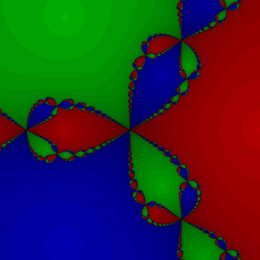
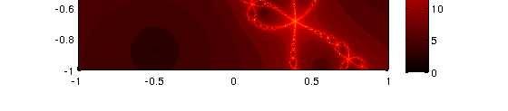
82