FALL UNIVERSITY OF NEVADA, LAS VEGAS DEPARTMENT OF MECHANICAL ENGINEERING MEG 421 Automatic Controls Design Project

Transcription

1 FALL UNIVERSITY OF NEVADA, LAS VEGAS DEPARTMENT OF MECHANICAL ENGINEERING MEG 421 Automatic Controls Design Project Objective: The design project will give everyone in the class an opportunity to apply the knowledge gained in class in a reasonably realistic setting. We will analyze plants, their dynamics and other properties, and explore design strategies by which we can create a good controller while considering the existing constraints. General Rules for all Reports As Seniors, you will be graduating soon. Prepare the reports as you would for a supervisor at your place of employment. Make the report as clear and transparent as possible. Graphs and Figures * Figure 1 DC Motor with limiter Every graph must have a descriptive Title. Label and Scale All axes. If a plot contains multiple lines, you must add a legend explaining each curve. Add handwritten legends if needed. Do NOT paste Matlab Scope images into the report, since they do not contain proper labeling. VisSim or Simulink Models: Avoid overlapping and crossing lines a much as possible. Re-arrange the icons so that a clear path from left to right is visible.

2 The schedule below lists due dates and assignments for the individual parts of the project. Due dates are Wednesdays of the week listed, before class. Due Week Topic date 7 Wed. 10/19 Report #1 Part 1: Model the plant assigned to you. Each plant has one input and one output variable. Choose state variables, create free-body diagrams, and determine the plant s differential equation in state variable form, see examples on pages 10 and 11. Express the plant model in transfer function form (by hand or better in Mathcad), and compute all plant poles. If your model is nonlinear, e.g. the independent variable comprises sinusoidal or quadratic terms, linearize the model equation about its operating point. Part 2: Model the complete linear open-loop system including the plant. Specify input and output variables, disturbances, and transfer functions. The complete open-loop system begins with a controller (model initially as gain K), followed by an amplifier (with limiter in the nonlinear case), the actuator = DC motor (see also second lab handout File: lab2v.pdf or the DC motor discussion in the textbook, Chapter 2), and the system being controlled. No sensor is specified. Assume that the controlled directly available to the controller. Select an appropriately sized DC servomotor (see instructions below) and amplifier to drive the plant. Part 3: Create a Linear open-loop computer model as seen in Fig. 1 below, where the plant is represented as the transfer function of part 1. Use VisSim or Simulink. Do not yet define the nonlinear elements (Limiter and Coulomb friction) shown in Fig. 1. Submit: 1. The complete validated model of your plant, including all free-body diagrams used to derive the state equations. Validation: Show that your plant is stable, i.e. that it has NO poles in the right half of the s-plane, see below. 2. The plant model in transfer function format, see example below. If you compute the transfer function and plant poles in Mathcad (RECOMMENDED) please include your Mathcad model in the report. 3. Verify that the model is open-loop stable by computing all plant poles. Submissions containing unstable plant poles are not accepted. List the Plant transfer function and all plant poles. Any undamped oscillators in the plant will result in imaginary axis pole pairs. However, if you discover unstable poles in the right half of the s-plane, please review your plant model for errors. All assigned plants are open-loop stable and therefore cannot have poles in the right half of the s-plane. 4. Validated VisSim or Matlab model, 5. a plot of the open-loop step response, in VisSim or Matlab. Please select the time scales so that both the transition and the steady state are visible. Again: Submissions containing system models with rhp poles will not be accepted.

3 10 11/02 Report #2 Part 1: Using the validated plant model of report 1, create a Nonlinear model VisSim or Simulink model only. Place the limiter after the amplifier, see Fig. 1. If a limiter is not explicitly given in the manufacturer s motor data sheet, choose it such that it limits the actuator output at approx. 70% of its maximum current. Part 2: Using a unit step reference input, design a P-controller for approx. 20% overshoot (if your plant is too poorly damped, document this fact and design for a larger overshoot. If your plant has imaginary axis poles, the closed loop may be unstable with P-control for any gain K. If the closed loop is unstable, demonstrate this fact by plotting the plant s root locus). Simulate and plot the feedback system step response with P-control for two scenarios: (a) Linear Model : No Limiter (b) Nonlinear Model with Limiter. Show the complete block diagram of both linear and nonlinear feedback systems. Verify that the loop has negative feedback. Also, compute and plot the closed loop system response to an appropriately sized disturbance step (r = 0). Place the disturbance between servo amplifier output and plant input, see Fig. 1.

4 Notes on defining the Limiter: Physical significance: The limiter models the fact that no real actuator can deliver infinite power. Check your motor specifications sheet for the input voltage range (typically +/- 10 Volts DC or similar). These values constitute the VOLTAGE LIMITER in Fig. 1. Your servo-amplifier will also have a current limit (max. current spec.) which you can enter in the model of Fig. 1 as a CURRENT LIMITER. Model the limiter in Matlab Simulink or VisSim. Limiter Dynamics: Try the limiter at different load levels. You ll observe that the control loop will be linear as long as the voltage input to the amplifier is within the the input voltage range (typically +/- 10 Volts DC or similar). Only when the voltage exceeds the limits will you see clipping. Run your simulations at step sizes large enough that clipping is visible. Graphing with Simulink: Use the SCOPE feature only while designing your control loop. For submission, connect the variables you wish to plot to a SIMOUT block (located in sinks). plot the results using the plot command. Please add a descriptive title to each plot, label all axes, and add legends whenever you plot multiple variables in the same plot. Use the Matlab legend or gtext command to label curves. Here is a Matlab code example that plots two responses from a simulink model ContinDiscrete.mdl. sim('contindiscrete') figure(1) plot(ycd(:,1),ycd(:,2),':') hold on plot(ycd(:,1),ycd(:,3)) xlabel('time (sec)'); ylabel(' responses'); title(' Responses of Continuous vs. Discrete Control') gtext('continuous controller') gtext('discrete controller, T =.07') grid on

5 1.4 Responses of Continuous vs. Discrete Control 1.2 continuous controller discrete controller, T =.07 1 responses Time (sec) Submit: Plant mathematical model and both VisSim or Matlab models (a) and (b) Plots: 1. Closed loop step responses for (a) and (b) in the same graph. 2. Closed loop disturbance responses for (a) and (b) in the same graph. For both plots, select the time scales so that both the transition and the steady state are visible. Re. Assignment #3: Show detail in all Root Locus plots, see examples below:

6 Never submit this: The poles and zeros near the origin are invisible. Better: Zoom in to show detail: 11 11/09 Report #3 Objective: Your task is to optimize your controller design to meet the following goals: reduce the steady state error as much as possible. Raise damping ζ to an optimum. Ideally ζ should be in the range from 0.5 to 0.7. Minimize the response time to reach the steady state value. You ll find that a compromise between these multiple goals will be necessary, and in some cases, you may not be able to meet all goals. Document your design choices and explain how you arrived at your final design. Procedure: Analyze the plant root locus, and design a compensator for the plant. The compensator may consist of any combination of the following: lead, lag, allpass filter. Simulate the feedback system step response with your compensator. The allpass filter can be of use to move conjugate complex pole pairs away from the imaginary axis. Important: Use the Matlab SISOTOOL to design lead, lag, and allpass filters. Design not merely for the specified overshoot, but also ensure that the steady state error is as small as possible. Start with the lead and/or allpass first. You can combine several

7 compensators, but remember that the number of compensator zeros must never exceed the number of compensator poles. Only after completing the lead/allpass design, add a lag filter if this is beneficial, i.e. if lag reduces the steady state error further. The lag pole should be close to the origin. Document the final design in your report, list all compensator poles and zeros, list the compensator transfer function, and plot the closed loop step response of the final design. Note: If your plant has two imaginary axis pole pairs, and if you cannot stabilize the closed loop with an allpass filter, you may add damping up to ζ = 0.2 to one of the pole pairs. Example: The model below contains two imaginary axis pole pairs in the first and third row equations. M1 s 2 + K x ( s) s x2 Fs ( ) ( s) 2 x3 0 M2 + K2 Add damping up to ζ = 0.2 to ONE row only. If you choose to add damping to the first row, compute damping coefficient B according to Chapter 3 (e.g. Equation 3.64). In the case of the row-1 pole pair, the equivalences are ω n = K 1 /M 1, and B/M 1 = 2ζ ω n, allowing the computation of B. The modified model would then result as: M1 s 2 + Bs + K1 10 s s s 2 M2 + K2 If you choose to alter the damping of one pole pair, document all steps of the process, compute the altered transfer function, including its open-loop poles and zeros. You should now be able to control the remaining single pole pair on the imaginary axis with a lead compensator. Describe and document clearly: plant and compensator transfer functions, definition of limiter, closed loop block diagrams. Document clearly the process by which you arrived at your choice of (lead and/or lag) compensator. Design the linear system first and document results in the first two plots. After completion of the compensator design, analyze the closed loop with the limiter and compare, in the third plot, the effect of the finite amplifier power on closed loop performance. Submit: - Plant mathematical model and VisSim or Matlab models - Plant transfer function and all plant poles. Plots: root locus of linear system incl. the final compensator Comparison: closed loop step responses with P-control (from project 2) vs. new compensator, both in same graph.. closed loop step responses (a)(linear) and (b)(nonlinear), both in same graph /16 Report #4 Analyze Plant Frequency response, design lead and/or lag and/or allpass compensator for the plant in the Bode plot. Simulate the feedback system step response with lead and/or lag control. Important: Use the Matlab SISOTOOL to design lead, lag, and allpass filters. Design not merely for the specified overshoot, but also ensure that the steady state error is as small as possible. Design using the lead and/or allpass first. You can combine several x1 x2 x3 0 Fs () 0

8 compensators, but remember that the number of compensator zeros must never exceed the number of compensator poles. Only after completing the lead/allpass design, add a lag filter if this is beneficial, i.e. if lag reduces the steady state error further.. The lag pole should be close to the origin. Document the final design in your report, list all compensator poles and zeros, list the compensator transfer function, and plot the closed loop step response of the final design. The Bode plot allows you to judge the effect of pole and zero placements better than the root locus plots. Place the compensator zero(s) such that you have an optimal phase margin at the gain crossover frequency. At the same time, the lead should be fast enough so that the magnitude plot crosses the 0-dB line as soon as possible. Describe and document clearly: plant and compensator transfer functions, definition of limiter, closed loop block diagrams. Document clearly the process by which you arrived at your choice of compensator. Design the linear system first and document results in the first two plots. After completion of the compensator design, add the limiter and compare, in the third plot, the effect of the finite amplifier power on closed loop performance. Submit: Plant mathematical model and VisSim or Matlab models Plots: Bode plots of linear system incl. the lead and/or lag compensator. Document how you chose the compensator, starting from the open-loop plant without lead and/or lag. After completing the design, show the Bode plot of the improved open-loop system including the lead and/or lag compensator and gain K of your choice. Comparison of (closed-loop) P-control vs. lead and/or lag control, both in same graph. closed loop step responses (a)(linear) and (b)(nonlinear), both in same graph /23 Final report: Review and finalize actuator needs. Review the actuator choice you made for report #1. Please recall that your actuator should deliver sufficient torque to deliver the same steady state response as the linear system. However, unlike the linear system which implicitly assumes an infinite power supply, use actual motor parameters from manufacturers specifications to select a motor/actuator that delivers the same steady state response as the linear system, but with power limited to perhaps 50% to 100% above the steady state power requirements. Define the limiter consistent with your DC motor and servo amplifier specifications. Document clearly how you transferred the DC motor specs to your block diagram. Define two realistic actuators (e.g. a marginal DC motor that can barely move the plant to the desired output value) and a large DC motor/servoamplifier (between 150% and 200% of the torque of the marginal design). Model both control loops with correctly defined output limiters. One design will deliver relatively low power and the other will deliver a faster response. Since actuators and servo amplifiers are typically expensive, present your supervisor two alternate design choices. Option 1 will normally be slower and less expensive. Option 2 will normally be faster and more costly. Submit: Plant mathematical model and VisSim or Matlab models, calculations of the limiter values for both actuator designs. Plot the following three closed loop system step responses in the same graph: (a) linear system step response, reflecting your best design. (b) both closed loop step responses for the two motor choices. (Include the spec sheets specifying motor torque constant and max. voltage/current). For the response plots, select the time scales so that both the transition and the steady state are visible.

9 Actuator selection for all plants: Build your model according to Fig. 1 in Matlab or Vissim. Use a DC Motor driven by a servo-amplifier to power all plants. You may initially use arbitrary values for the motor parameters. Add a plot to the output variable (output vs. time), apply perhaps an input voltage of 10V to the motor, and observe the output as you vary the motor torque constant, K t. Now modify the motor torque constant such that the motor can displace the output variable (by +/- 0.1m for translation type output), (or by +/- 0.5 radians if the output an angle) exhibits a rise time (see Chapter 3.4 for definitions) of about 300 ms or less. For systems with large masses or inertiae, slower step responses are in order, so use your judgment on what would constitute a reasonable motor choice in the context of your assignment. Using the servomotor vendor specs on the web, locate a motor that approximately meets the requirements. All servomotors require a servo-amplifier. The servo-amplifier is shown as gain K amp in Fig. 1. The servo-amplifier supplies the variable power requested by the controller. Select the servo-amplifier so that it matches approximately the motor specifications. You are free to select any real K t and V armature. Document your motor selection (URL and printout of motor specs). Identify an industrial motor that closely meets your application s requirements. You can find DC servomotor vendors on the web. See for instance: Include the motor selection and its list of parameters in report #1. Motor Dynamics Model: Follow example 2.11 in Franklin s book. The output of the motor is the torque τ(t). The standard DC servomotor model also contains a back-emf or speed voltage. You should neglect the back-emf because the motor speed is normally small. The transfer function for a voltage input and torque output now results as a first order term. If the motor is rigidly coupled to the first mass or inertia, simply add the motor inertia or its mass equivalent to the first dynamic element of your plant. Controller (model initially as gain, later as R(s) Lead controller) Volt age Controller K amp Actuator (model armature part of servo motor) Voltage Limiter Motor: K t /(Ls+R) Cur rent Current Limiter W(s) Disturbance Plant Y(s) Fig. 1 Motor Dynamics Model with Limiter(s)

10 Report #1: Developing the system model 1. Perform a free-body analysis for each inertia or mass. Remember: action = reaction, and make sure that the signs for springs and dampers are correct. See example at left. Make sure that all coupled springs and dampers respond correctly. For instance, if inertia J1 is coupled by a tension spring to mass M, the spring force must increase as the distance between J1 and M increases. 2. Apply Newton s law to each free-body mass/inertia. 3. Write your differential equation in matrix form, and use Laplace notation. Solving determinants and sorting terms is easiest in Mathcad. Use the symbolics menu. See also example below. 4. Your transfer function then results as output(s)/input(s), by applying Cramer s rule. Verify the open-loop stability of your plant by computing ALL plant poles. If you find any unstable poles, your model contains errors which you should correct before submitting the report. J 1 J text J 1 text 2 Start with the mass or inertia to which the external force/torque is applied. Here: Start with J 1 ω 2, θ 2 ω 1, θ 1 M A Inertia J 2 Force F Reaction is equal and opposite to the one at J 1 A Force F Load Torque r Inertia J 1 Reactions Reactions at J 2 : equal and Opposite to J 1 r Mass M Translation B Sample sixth-order Dynamics Model in Free-Body Analysis Matrix form, using Laplace notation: (done in Mathcad)

11 Sample Computation of the Plant poles (roots of the char. Equation) in Mathcad. You can use any other suitable software, e.g. Matlab. The char. Equation is shown below, note the bold = sign. In Mathcad, place cursor on the s-variable, then select Symbolics Variable Solve. The resulting solution vector is shown below. This plant is stable (no real parts > 0) Example: The Characteristic Equation: e-10s s s s s s has roots (poles) at: i Procedures: A progress report is due on each date listed. 2.24i 10 1

12 2. Use either VisSim or Matlab. You will be required to model linear as well as nonlinear systems. 3. Deliverables for each report include: Mathematical analysis, e.g. transfer functions, poles and zeros (linear model only). A plot of each VisSim or Simulink model used. Step response and other plots as specified in the schedule above. Use a report format similar to the format for the lab. See Individual assignments are listed below. Name Remarks Plant Schematic x 3 Albright,Jacob B

13 y Avelar,Lisett N Benavente,Ja mes Input is force Ft). is x 3 (t) = position of the last car relative to the middle car. K= 10 4 N/m/ B = 2*10 2 Ns/m M = 4500 kg, m= kg x 2 Bergstrom,Tre vor J

14 Boles,Jeremia h θ = angle of rotation of beam J1 Spring Ks2 is unstretched at θ = 0. Assume that the angle θ is small and use linear approximati ons for sinθ or tanθ θ 1 Lever-Spring System. Input var: F1 = Force applied to Mass M1 in +x1- direction (down). Spring Stiffness 1 Ks1 80 N/m Spring Stiffness 2 Ks2 400 N/m, attached to ground Damping Coefficient Kd1 120 N s/m Rotational Inertia J1 12 Kg m^2 Mass of Block M1 15 Kg Distance from Fulcrum to Left End of Rod R1 = 0.3 m Distance from Fulcrum to Right End of Rod R2 = 0.7 m Bou Abdo, Rawad T ω 3 = angular velocity of the gear at θ 3 Brown,Robert J

15 ω 2 (t) angular velocity at θ 2 Burton,Mitchell P Data: Input is torque T(t) applied at J 1. θ 3 (t) Chagin Sanchez,Step hanie M

16 Charnkijtawaru sh,chanatan Input T(t), is x1(t) Christy,Jessic a M Conlin,Geoffre y M Active Suspension : A disturbance at B (change of terrain elevation z(t)) causes the cart to tilt. Control elevation y1 such that y1 = y2 Model the rotation θ(t) using a single constant inertia

17 Input F(t), θ(t),small angles Eckstein,Sally Fitzjerrells,Ale xander R

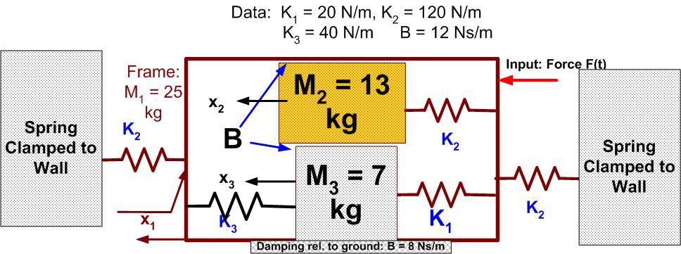
18 Input is force F(t). X 2 (t) Fjare,Paul D Frappier,Ann M Input is force F(t). x (t) = displacement of mass M. Inertia J is rolling only, no slipping relative to mass M. Spring K2 is attached to center of Inertia J1.

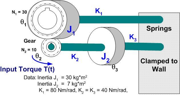
19 Input is force F(t). y (t) = displacement of mass m2. Inertia J1 is rolling only, no slipping relative to mass m2. Spring K3 is attached to center of Inertia J1. Data: Galli,Justin J 1 = 25 kgm 2, K 1 = K 2 =20 N/m, K 3 = 50 Nm/rad, b = 8 Ns/m, m1 = 15 kg m2 = 30 kg, r1= 1.5 m r2 = 0.3 m θ Ghanaatrad,R yan B

20 Input is force F(t). x (t) Gonzalez,Enri que L Input is torque T(t). Radius of Pulley : R = 0.5 m Hart,Dustin T Input is Force F(t) Pure rotation at inertia A. Center of A does not move. Hartman,Jessi ca N Herrera,Joshu a William Input is torque T(t). θ 4 N1 through N4 are the number of gear teeth given as: 12, 16, 20, 30 K 1 = 20 N/m, K 2 =30 Nm/rad, D = 50 Ns/m

21 Data: J 5 = J 6 = 20 kg-m 2, J 1 = J2 = J 3 = J4 gears 1 through 4 inertia = 0.7 kg m 2 K 1 Input is torque T(t). x(t) k = 25 Nm/rad Lennon,Derek Litton,Kyle Torsional spring between N4 and Pinion gear: k = 19 Nm/rad Inertia at Pinion: J 4 = 4 kg-m 2 Force input is applied to right of uniform plate B, with dimensions 2m by 1.5 m. We wish to maintain the angle of rotation of B at zero. A unit disturbance step is applied at t=0 to the left side of plate B.

22 Input is armature voltage e a (t). x(t) Torsional spring between N2 and gear: k = 12 Nm/rad Inertia of Pinion Gear: J Gear = 12 kgm 2 k = 12 Nm/rad Magann,Brian Input is force f(t). x 2 (t) Monsalud,Dha ryl

23 y Mun,Bongjun Input is torque τa(t). x 3 (t) Nelson,Shelby E Data: J = 12 kg-m 2, K 1 = 25 Nm/rad, B = 20 Ns/m K 2 = K 3 =40 N/m R= 0.7 m, M= 30 kg

24 Input is torque τa(t). x(t) Data: J1 = 18 kgm 2, J2 = 25 kgm 2, K 1 = 20 Nm/rad, B = 30 Nms/rad K 2 = 35 N/m R= 0.5 m, M= 25 kg Orr,Katelyn Input T(t), θ 2 (t) Oslinker,Brian Matthew

25 θ1(t) Poblete,Jonath an A Input is torque T(t). angular velocity ω 1 k = 20 Nm/rad Poon,Tik Ho Torsional spring between N1 and inertia to its left: k = 20 Nm/rad θ k = 20 Nm/rad Pratt,Timothy N

26 Input is torque T(t). y Radius of inertia J 2 : R= 0.5 m Pulido,Jorge L θ Friction between Inertia J and Ground: B_ trans = 7 Ns/m Raj,Praveen θ Torsional Damping of Pendulum: B = 3 Nms/rad Rebman,Kyle W

27 Reyburn,Matth ew H θ 2 Richardson IV,Norman E Input is force F(t). X 1 (t) = displacement of mass M 2. Ross,Stephani e

28 Ross,Tim W Assume small angles of rotation. Santos,Ronnie G

29 Schweter,Jona than M Ks1 = 15 N/m Kd2 = 8 Ns/m Silva,Daniel F

30 Smith,Allan M Input is torque T(t). θ 3 (t) Stern,Jeremy T Sun,Hai Rui Contact Dr. Mauer for assignment

31 Viscous damping B is present in both inertiae J1 and J2: B = 20 Nms/rad Trabia,Sarah S Triay,Jose R Input is disturbance h(t) (road roughness) body tilt angle θ(t). Wheels are attached to Vargas,Sylvest the car mass through er Lirio spring and Data: M-body = 1200 kg, car body radius of gyration k = 1m C f = 2500 Ns/m C r = 2000 Ns/m, K f = =28000 N/m k r = N/m L f =0.9 m, L r =1.2 m

32 damper. Use 2 wheels. M wheel = 25 kg Do not consider tire inertia. Suspension elasticity and damping are modeled by K and C as shown in the illustration Verdin,Bruno H Wheeler,Britta ny

33 Input torque T(t) is applied at θ 2. Gear at θ 2 has no Inertia. θ 1 Damping at J2 is B = 7 Nms/rad Wu,Soloman G θ A Zeng,Zheng