The Root Locus Method
|
|
|
- Thomasine Charles
- 5 years ago
- Views:
Transcription
1 The Root Locu Method MEM 355 Performance Enhancement of Dynamical Sytem Harry G. Kwatny Department of Mechanical Engineering & Mechanic Drexel Univerity
2 Outline The root locu method wa introduced by Evan in the It remain a popular tool for imple SISO control deign. What i a root locu? Pole & Tranient Repone (Why do we care about pole?) The Root Locu Method Problem Definition The Two Key Formula Root Locu Rule Example: Flexible Spacecraft Robotic Arm General Aviation Aircraft Helicopter Pitch Control
3 Deigning a Feedback Control Sytem Firt we chooe a compenator There are many ueful compenator type.we have already een Proportional and Proportional plu Integral. Thi give u a tructure, i.e., a compenator tranfer function. The tranfer function will have one or more free parameter. The root locu method i one approach to elect the free deign parameter o a to achieve deired tranient behavior.
4 What i a Root Locu? On the right i a negative feedback loop We wih to examine the cloed loop pole a the gain K varie A K increae from zero the 4 pole move from the open loop value & trace 4 loci At any particular value of K there are 4 cloed loop pole In thi example there i a critical value of K at which the ytem become untable. y ye - K = K = 0 G () H( ) ( + 3) ( + 1)( + )( + 4) ( + 1)( + )( + 4) G H = K G 1 = = GH K + 3K Im at K critical y Re tability i lot
5 Uing Matlab >> =tf(''); >> G=(+3)/(*(+1)*(+)*(+4)); >> rlocu(g) >> grid >> [K,Pole]=rlocfind(G) Select a point in the graphic window elected_point = i K = Pole = i i i i -1-1 ) Imaginary Axi (econd Root Locu Real Axi (econd -1 )
6 Example ( + 1) 1, 1 CL 1 ( + 1) 1 + K + K G G = K H = G = + G 1+ G = 1+ K = K + K = = K ± K K Im K = K = K = 4 K = 0 Re
7 Tranient Repone Conider a ytem decribed by the open loop tranfer function n G K c pfd 1 = d + λ1 There are three way to ae ytem tranient behavior: 1. time domain (output time trajectorie). pole (or eigenvalue) location 3. frequency repone (Bode or Nyquit plot) Here we conider pole location. The pole are the root of c The root locu method i concerned with adjuting the cloed loop pole poition ( ρω 1 1 ω1 ) ( ρpωp ωp)( λ1) ( λq) d = = 0 Complex root occur in complex conjugate pair. In thi cae there are p+q pole
8 Ideal Pole Location Im α degree of tability, decay rate 1/α ideal region for cloed loop pole θ damping ratio θ = in 1 ρ Re Our goal i to deign a compenator o that the cloed loop pole lie in the haded region. We get to chooe the form of the compenator and elect it parameter.
9 Problem Definition The cloed loop input repone tranfer function i G yy ( ) G = 1 + GH The error repone tranfer function i (recall e= y y) 1+ GH G Ge( ) = 1 Gy( ) = 1+ GH The pole of the cloed loop ytem are the root (zero) of y - G () H( ) y 1+ GH( ) = 0
10 Problem Definition, Cont d Suppoe ( m ) n z z + b + + b G( ) H( ) = K = K = K d p p + a + + a m m 1 1 m 1 0 n n 1 1 n n 1 0 n, d are completely known, but K i a parameter that we can adjut. Root Locu Problem: Generate a ketch in the complex plane of with varying gain K. the cloed loop pole
11 Solution Strategie We will do thi two way: The eay way: Have MATLAB olve for the root for each of a pecified lit of value for K and plot them. The hard (old) way: Generate a ketch by hand. Why do it the hard way at all? We need to know how to interpret the plot. We obtain inight concerning the choice of compenator. We learn how to et the compenator parameter other than the gain K.
12 Root Locu Method ~ 1 Magnitude equation d() + Kn() 1+ G ( ) H ( ) = 0 = 0 d() + Kn() = 0 d () n () j(k+ 1) π 1+ G( ) H( ) = 0 K = 1 = e, k = 0, ± 1, ±, d () Thi mean n () n () K = 1 and K = (k+ 1) π d () d () for K 0 : K n () n () = 1 and = (k+ 1) π d () d () Angle equation
13 Root Locu Method ~ Our goal i to find value of that atify both of thee equation. Note that for any given, the magnitude equation i atified for ome value of K, i.e., K = d n Note that the angle equation doe not depend on K at all. Strategy: Firt, find value of that atify the angle equation. Second, calibrate the plot uing the magnitude equatio n.
14 Root Locu ~ 3 Uing the Angle Formula G H = ( + 3)( + 4) ( + 1)( + ) tet point = + j3 Im n () = (k + 1) π d () n d = (k+ 1) π θ 4 θ 3 θ θ ( k ) Re θ + θ θ + θ = π for any integer = + j3 i not a point on the root locu The point = + i / i θ + θ θ + θ = 180 k
15 Baic Rule ~ 1 1. Number of branche: The number of branche of the root locu equal the number of open loop pole. + i the order of theorder of the polynomial d Kn d. Symmetry: The root locu i ymmetric about the real axi. Pole occur in complex conjugate pair. 3. Starting & ending point: The root locu begin at the open loop pole and end at the finite and infinite open loop d + Kn = 0 d =0 a K 0 1 K 0 zero. d + n = n =0 a K if i bounded
16 Example: ( + 3) ( + 1)( + )( + 4) G H = K Im Re
17 Baic Rule ~ 4. Real-axi egment: For K > 0, real axi egment to the left of an odd number of finite real axi pole and/or zero are part of the root locu. Im θ θ Re Tet point 1
18 Baic Rule ~ 3 5. Behavior at infinity: The root locu approache infinity along aymptote with angle: (k + 1) π θ =, k = 0, ± 1, ±, ± 3, # finite pole # finite zero Furthermore, thee aymptote interect the real axi at a common point given by σ = finite pole finite zero # finite pole # finite zero
19 Baic Rule ~ 4 Angle part i eay: n m = i= 1 i i= 1 d n ( z ) ( p ) jθ Take = ρe. For ρ, λ = θ Then m n z p mθ nθ i= 1 i i= 1 n So = ( k+ 1) π ( m n) θ = ( k+ 1) π d i i i
20 Baic Rule ~ 4 6. Real axi breakaway and break-in point: The root locu break away from the real axi where the gain i a (local) maximum on the real axi, and break into the real axi where it i a local minimum. To locate candidate break point d imply plot K( ) = on the axi egment n d d or olve = 0 d n 7. jω-axi croing: Ue Routh tet to determine value of K for which loci cro imaginary axi.
21 Routh Stability Tet It i deired to determine the number of right hand plane root of a polynomial, ay: a a0 3 a3 a a + a + a+ a = a a0 3 a3 a1 0 b1 b b3 1 c1 c 0 d1 b a3 a3 c 1 1 a 1 a0 a a a 0 =, b =,... = a b a 3 1 b 1 3,... The number of right half plane pole i equal to the number of ign change in the firt column. a
22 Uing MATLAB The baic MATLAB function are: rlocu rlocu(y) calculate and plot the root locu of the open-loop SISO model y. rlocfind [K,POLES] = RLOCFIND(SYS) i ued for interactive gain election from the root locu plot of the SISO ytem SYS generated by RLOCUS. RLOCFIND put up a crohair curor in the graphic window which i ued to elect a pole location on an exiting root locu. The root locu gain aociated with thi point i returned in K and all the ytem pole for thi gain are returned in POLES. iotool When invoked without input argument, iotool open a SISO Deign GUI for interactive compenator deign. Thi GUI allow you to deign a ingle-input/ingle-output (SISO) compenator uing root locu and Bode diagram technique.
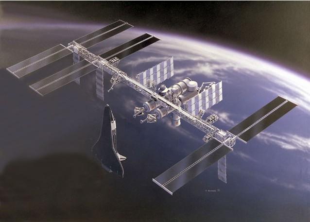
23 Flexible Spacecraft
24 Flexible Spacecraft Θ K G H Θ = = K ( + 4)( + + ) ( + + 1) ( + 4)( + 1± j) ( ± 0.866) K j 1 4 With One Flex Mode Rigid = Θ + 4 G H K K + 4 Θ
25 Spacecraft = dcl 1 K 1 6K 10K 8K K K 1+ 3 K K 10 0 Rigid Im Re K + 6K 1+ K ( + ) K 1 3K 6K 8K 1 3K + 6K + K K + K 1 3K + 6K 1 0, 3 6 0, 0 8K 0 0 Alway poitive (prove it) One Flex Mode Im Re untable egment
26 Example Robotic Arm Compenator Amplifier Motor/ Speed Controller Θ K Θ G = 0K = 0K ( + 4)( ) ( + 4)( + 5.5)
27 Robotic Arm Im Im Re Re? Im 45, 135, 5, Re
28 Robotic Arm 3 Plot K d =, 4, 0.1 n Max, breakaway point at K Min, breakin point at
29 Robotic Arm 4 >> =tf(''); >> G=0*(+0.1)/(^*(+4)*(+5.5)^); >> rlocu(g) >> rlocfind(g) Select a point in the graphic window elected_point = i an =.111 elected_point = i an =
30 Robotic Arm 5 G cl = ( + ) 0K K K Routh Table K K K K K K 89.76K K K Governing Inequality , , 0 K > K K > K > 11 K < = K < =
 θ elevator angle, δ ( ) Plant: G = 160 p Lead")
 ( + 5+ 40)( + 0.03+ 0.")
31 Example: Piper Dakota Pitch Control e, error θ - G c δ e G ( p ) θ elevator angle, δ ( ) Plant: G = 160 p Lead compenator: G e pitch angle, θ ( +.5)( + 0.7) ( )( ) c ( ) + 3 = K + 0 Franklin & Powell 3 rd Ed
32 Piper Dakota Im What do we expect? Im Re Re
33 Piper Dakota >> =tf(''); >> Gp=160*(+.5)*(+0.7)/((^+5*+40)*(^+0.03*+0.06)); >> Gc=(+3)/(+0); >> G=Gc*Gp; >> rlocu(g) >> grid >> [K,Pole]=rlocfind(G) Select a point in the graphic window elected_point = i K = Pole = i i i i >> Gcl=1.5*G/(1+1.5*G); >> tep(gcl)
34 Piper Dakota

35 Piper Dakota Open loop repone to elevator Cloed loop repone with: K = 1.5
 tabilizer + 1 K Pick the inner loop pitch control + 9 gain K o that the dominant inner loop pole have a damping ratio of 0.707.")
36 Example: Helicopter Pitch Control Notice untable dynamic pilot diturbance helicopter - K ( + ) ( + 0.4)( ) tabilizer + 1 K Pick the inner loop pitch control + 9 gain K o that the dominant inner loop pole have a damping ratio of Select an outer loop gain (tick enitivity) to place the pole. Determine ultimate error in repone to unit tep diturbance.
37 Inner (Stabilization) Loop 1+ GH = 1+ K ( ) ( + 0.4)( ) ( ) ( + 9) The inner loop root locu i hown on the right. Chooe a gain K = 1.5. The inner loop reolve to: G ( ) Gp = GG = c p 5( )( + 9) ( ± j3.53)( )( )
38 Outer Loop Deign pilot Inner loop - K ( )( + 9) ( ± j3.53)( )( )
39 Outer Loop On the bai of the root locu on the right, chooe a gain of 1. The cloed loop pole are: ± j ± j
40 Diturbance Repone Error G de G = 1 + G = pilot G 5( )( + 9) ( )( ± j3.50)( ± j0.646)( ) 1 lim Gde =
41 Summary How pole characterize tranient repone Oberving the influence of gain on cloed loop pole uing root locu plot Sketching the root locu: The magnitude and gain formula Baic rule of root locu ketching Uing MATLAB Example
MEM 355 Performance Enhancement of Dynamical Systems Root Locus Analysis
 MEM 355 Performance Enhancement of Dynamical Sytem Root Locu Analyi Harry G. Kwatny Department of Mechanical Engineering & Mechanic Drexel Univerity Outline The root locu method wa introduced by Evan in
ME2142/ME2142E Feedback Control Systems
 Root Locu Analyi Root Locu Analyi Conider the cloed-loop ytem R + E - G C B H The tranient repone, and tability, of the cloed-loop ytem i determined by the value of the root of the characteritic equation
Root Locus Contents. Root locus, sketching algorithm. Root locus, examples. Root locus, proofs. Root locus, control examples
 Root Locu Content Root locu, ketching algorithm Root locu, example Root locu, proof Root locu, control example Root locu, influence of zero and pole Root locu, lead lag controller deign 9 Spring ME45 -
Chapter 7. Root Locus Analysis
 Chapter 7 Root Locu Analyi jw + KGH ( ) GH ( ) - K 0 z O 4 p 2 p 3 p Root Locu Analyi The root of the cloed-loop characteritic equation define the ytem characteritic repone. Their location in the complex
EE Control Systems LECTURE 14
 Updated: Tueday, March 3, 999 EE 434 - Control Sytem LECTURE 4 Copyright FL Lewi 999 All right reerved ROOT LOCUS DESIGN TECHNIQUE Suppoe the cloed-loop tranfer function depend on a deign parameter k We
CISE302: Linear Control Systems
 Term 8 CISE: Linear Control Sytem Dr. Samir Al-Amer Chapter 7: Root locu CISE_ch 7 Al-Amer8 ١ Learning Objective Undertand the concept of root locu and it role in control ytem deign Be able to ketch root
MODERN CONTROL SYSTEMS
 MODERN CONTROL SYSTEMS Lecture 1 Root Locu Emam Fathy Department of Electrical and Control Engineering email: emfmz@aat.edu http://www.aat.edu/cv.php?dip_unit=346&er=68525 1 Introduction What i root locu?
Root Locus Diagram. Root loci: The portion of root locus when k assume positive values: that is 0
 Objective Root Locu Diagram Upon completion of thi chapter you will be able to: Plot the Root Locu for a given Tranfer Function by varying gain of the ytem, Analye the tability of the ytem from the root
Control Systems Analysis and Design by the Root-Locus Method
 6 Control Sytem Analyi and Deign by the Root-Locu Method 6 1 INTRODUCTION The baic characteritic of the tranient repone of a cloed-loop ytem i cloely related to the location of the cloed-loop pole. If
Delhi Noida Bhopal Hyderabad Jaipur Lucknow Indore Pune Bhubaneswar Kolkata Patna Web: Ph:
 Serial :. PT_EE_A+C_Control Sytem_798 Delhi Noida Bhopal Hyderabad Jaipur Lucknow Indore Pune Bhubanewar olkata Patna Web: E-mail: info@madeeay.in Ph: -4546 CLASS TEST 8-9 ELECTRICAL ENGINEERING Subject
Automatic Control Systems. Part III: Root Locus Technique
 www.pdhcenter.com PDH Coure E40 www.pdhonline.org Automatic Control Sytem Part III: Root Locu Technique By Shih-Min Hu, Ph.D., P.E. Page of 30 www.pdhcenter.com PDH Coure E40 www.pdhonline.org VI. Root
Lecture 12: Examples of Root Locus Plots. Dr. Kalyana Veluvolu. Lecture 12: Examples of Root Locus Plots Dr. Kalyana Veluvolu
 ROOT-LOCUS ANALYSIS Example: Given that G( ) ( + )( + ) Dr. alyana Veluvolu Sketch the root locu of 1 + G() and compute the value of that will yield a dominant econd order behavior with a damping ratio,
Chapter 13. Root Locus Introduction
 Chapter 13 Root Locu 13.1 Introduction In the previou chapter we had a glimpe of controller deign iue through ome imple example. Obviouly when we have higher order ytem, uch imple deign technique will
Control Systems. Root locus.
 Control Sytem Root locu chibum@eoultech.ac.kr Outline Concet of Root Locu Contructing root locu Control Sytem Root Locu Stability and tranient reone i cloely related with the location of ole in -lane How
Control Systems. Root locus.
 Control Sytem Root locu chibum@eoultech.ac.kr Outline Concet of Root Locu Contructing root locu Control Sytem Root Locu Stability and tranient reone i cloely related with the location of ole in -lane How
CONTROL SYSTEMS. Chapter 5 : Root Locus Diagram. GATE Objective & Numerical Type Solutions. The transfer function of a closed loop system is
 CONTROL SYSTEMS Chapter 5 : Root Locu Diagram GATE Objective & Numerical Type Solution Quetion 1 [Work Book] [GATE EC 199 IISc-Bangalore : Mark] The tranfer function of a cloed loop ytem i T () where i
Linear System Fundamentals
 Linear Sytem Fundamental MEM 355 Performance Enhancement of Dynamical Sytem Harry G. Kwatny Department of Mechanical Engineering & Mechanic Drexel Univerity Content Sytem Repreentation Stability Concept
Control Systems Engineering ( Chapter 7. Steady-State Errors ) Prof. Kwang-Chun Ho Tel: Fax:
 Prof. Kwang-Chun Ho Tel: Fax:") Control Sytem Engineering ( Chapter 7. Steady-State Error Prof. Kwang-Chun Ho kwangho@hanung.ac.kr Tel: 0-760-453 Fax:0-760-4435 Introduction In thi leon, you will learn the following : How to find the
Control Sytem Engineering ( Chapter 7. Steady-State Error Prof. Kwang-Chun Ho kwangho@hanung.ac.kr Tel: 0-760-453 Fax:0-760-4435 Introduction In thi leon, you will learn the following : How to find the
ME 375 FINAL EXAM SOLUTIONS Friday December 17, 2004
 ME 375 FINAL EXAM SOLUTIONS Friday December 7, 004 Diviion Adam 0:30 / Yao :30 (circle one) Name Intruction () Thi i a cloed book eamination, but you are allowed three 8.5 crib heet. () You have two hour
Stability. ME 344/144L Prof. R.G. Longoria Dynamic Systems and Controls/Lab. Department of Mechanical Engineering The University of Texas at Austin
 Stability The tability of a ytem refer to it ability or tendency to eek a condition of tatic equilibrium after it ha been diturbed. If given a mall perturbation from the equilibrium, it i table if it return.
Homework 12 Solution - AME30315, Spring 2013
 Homework 2 Solution - AME335, Spring 23 Problem :[2 pt] The Aerotech AGS 5 i a linear motor driven XY poitioning ytem (ee attached product heet). A friend of mine, through careful experimentation, identified
Figure 1: Unity Feedback System
 MEM 355 Sample Midterm Problem Stability 1 a) I the following ytem table? Solution: G() = Pole: -1, -2, -2, -1.5000 + 1.3229i, -1.5000-1.3229i 1 ( + 1)( 2 + 3 + 4)( + 2) 2 A you can ee, all pole are on
Feedback Control Systems (FCS)
") Feedback Control Sytem (FCS) Lecture19-20 Routh-Herwitz Stability Criterion Dr. Imtiaz Huain email: imtiaz.huain@faculty.muet.edu.pk URL :http://imtiazhuainkalwar.weebly.com/ Stability of Higher Order
Feedback Control Sytem (FCS) Lecture19-20 Routh-Herwitz Stability Criterion Dr. Imtiaz Huain email: imtiaz.huain@faculty.muet.edu.pk URL :http://imtiazhuainkalwar.weebly.com/ Stability of Higher Order
376 CHAPTER 6. THE FREQUENCY-RESPONSE DESIGN METHOD. D(s) = we get the compensated system with :
 = we get the compensated system with :") 376 CHAPTER 6. THE FREQUENCY-RESPONSE DESIGN METHOD Therefore by applying the lead compenator with ome gain adjutment : D() =.12 4.5 +1 9 +1 we get the compenated ytem with : PM =65, ω c = 22 rad/ec, o
376 CHAPTER 6. THE FREQUENCY-RESPONSE DESIGN METHOD Therefore by applying the lead compenator with ome gain adjutment : D() =.12 4.5 +1 9 +1 we get the compenated ytem with : PM =65, ω c = 22 rad/ec, o
ROOT LOCUS. Poles and Zeros
 Automatic Control Sytem, 343 Deartment of Mechatronic Engineering, German Jordanian Univerity ROOT LOCUS The Root Locu i the ath of the root of the characteritic equation traced out in the - lane a a ytem
SKEE 3143 CONTROL SYSTEM DESIGN. CHAPTER 3 Compensator Design Using the Bode Plot
 SKEE 3143 CONTROL SYSTEM DESIGN CHAPTER 3 Compenator Deign Uing the Bode Plot 1 Chapter Outline 3.1 Introduc4on Re- viit to Frequency Repone, ploang frequency repone, bode plot tability analyi. 3.2 Gain
The state variable description of an LTI system is given by 3 1O. Statement for Linked Answer Questions 3 and 4 :
 CHAPTER 6 CONTROL SYSTEMS YEAR TO MARKS MCQ 6. The tate variable decription of an LTI ytem i given by Jxo N J a NJx N JN K O K OK O K O xo a x + u Kxo O K 3 a3 OKx O K 3 O L P L J PL P L P x N K O y _
EE Control Systems LECTURE 6
 Copyright FL Lewi 999 All right reerved EE - Control Sytem LECTURE 6 Updated: Sunday, February, 999 BLOCK DIAGRAM AND MASON'S FORMULA A linear time-invariant (LTI) ytem can be repreented in many way, including:
Stability Criterion Routh Hurwitz
 EES404 Fundamental of Control Sytem Stability Criterion Routh Hurwitz DR. Ir. Wahidin Wahab M.Sc. Ir. Arie Subiantoro M.Sc. Stability A ytem i table if for a finite input the output i imilarly finite A
March 18, 2014 Academic Year 2013/14
 POLITONG - SHANGHAI BASIC AUTOMATIC CONTROL Exam grade March 8, 4 Academic Year 3/4 NAME (Pinyin/Italian)... STUDENT ID Ue only thee page (including the back) for anwer. Do not ue additional heet. Ue of
Module 4: Time Response of discrete time systems Lecture Note 1
 Digital Control Module 4 Lecture Module 4: ime Repone of dicrete time ytem Lecture Note ime Repone of dicrete time ytem Abolute tability i a baic requirement of all control ytem. Apart from that, good
NAME (pinyin/italian)... MATRICULATION NUMBER... SIGNATURE
... MATRICULATION NUMBER... SIGNATURE") POLITONG SHANGHAI BASIC AUTOMATIC CONTROL June Academic Year / Exam grade NAME (pinyin/italian)... MATRICULATION NUMBER... SIGNATURE Ue only thee page (including the bac) for anwer. Do not ue additional
POLITONG SHANGHAI BASIC AUTOMATIC CONTROL June Academic Year / Exam grade NAME (pinyin/italian)... MATRICULATION NUMBER... SIGNATURE Ue only thee page (including the bac) for anwer. Do not ue additional
Lecture 8. PID control. Industrial process control ( today) PID control. Insights about PID actions
 PID control. Insights about PID actions") Lecture 8. PID control. The role of P, I, and D action 2. PID tuning Indutrial proce control (92... today) Feedback control i ued to improve the proce performance: tatic performance: for contant reference,
Lecture 8. PID control. The role of P, I, and D action 2. PID tuning Indutrial proce control (92... today) Feedback control i ued to improve the proce performance: tatic performance: for contant reference,
Lecture 4. Chapter 11 Nise. Controller Design via Frequency Response. G. Hovland 2004
 METR4200 Advanced Control Lecture 4 Chapter Nie Controller Deign via Frequency Repone G. Hovland 2004 Deign Goal Tranient repone via imple gain adjutment Cacade compenator to improve teady-tate error Cacade
Wolfgang Hofle. CERN CAS Darmstadt, October W. Hofle feedback systems
 Wolfgang Hofle Wolfgang.Hofle@cern.ch CERN CAS Darmtadt, October 9 Feedback i a mechanim that influence a ytem by looping back an output to the input a concept which i found in abundance in nature and
Chapter #4 EEE Automatic Control
 Spring 008 EEE 00 Chapter #4 EEE 00 Automatic Control Root Locu Chapter 4 /4 Spring 008 EEE 00 Introduction Repone depend on ytem and controller parameter > Cloed loop pole location depend on ytem and
Digital Control System
 Digital Control Sytem - A D D A Micro ADC DAC Proceor Correction Element Proce Clock Meaurement A: Analog D: Digital Continuou Controller and Digital Control Rt - c Plant yt Continuou Controller Digital
Given the following circuit with unknown initial capacitor voltage v(0): X(s) Immediately, we know that the transfer function H(s) is
: X(s) Immediately, we know that the transfer function H(s) is") EE 4G Note: Chapter 6 Intructor: Cheung More about ZSR and ZIR. Finding unknown initial condition: Given the following circuit with unknown initial capacitor voltage v0: F v0/ / Input xt 0Ω Output yt -
EE 4G Note: Chapter 6 Intructor: Cheung More about ZSR and ZIR. Finding unknown initial condition: Given the following circuit with unknown initial capacitor voltage v0: F v0/ / Input xt 0Ω Output yt -
ECE 3510 Root Locus Design Examples. PI To eliminate steady-state error (for constant inputs) & perfect rejection of constant disturbances
 & perfect rejection of constant disturbances") ECE 350 Root Locu Deign Example Recall the imple crude ervo from lab G( ) 0 6.64 53.78 σ = = 3 23.473 PI To eliminate teady-tate error (for contant input) & perfect reection of contant diturbance Note:
ECE 350 Root Locu Deign Example Recall the imple crude ervo from lab G( ) 0 6.64 53.78 σ = = 3 23.473 PI To eliminate teady-tate error (for contant input) & perfect reection of contant diturbance Note:
ME 375 FINAL EXAM Wednesday, May 6, 2009
 ME 375 FINAL EXAM Wedneday, May 6, 9 Diviion Meckl :3 / Adam :3 (circle one) Name_ Intruction () Thi i a cloed book examination, but you are allowed three ingle-ided 8.5 crib heet. A calculator i NOT allowed.
Linear-Quadratic Control System Design
 Linear-Quadratic Control Sytem Deign Robert Stengel Optimal Control and Etimation MAE 546 Princeton Univerity, 218! Control ytem configuration! Proportional-integral! Proportional-integral-filtering! Model
Lecture 10 Filtering: Applied Concepts
 Lecture Filtering: Applied Concept In the previou two lecture, you have learned about finite-impule-repone (FIR) and infinite-impule-repone (IIR) filter. In thee lecture, we introduced the concept of filtering
1 Routh Array: 15 points
 EE C28 / ME34 Problem Set 3 Solution Fall 2 Routh Array: 5 point Conider the ytem below, with D() k(+), w(t), G() +2, and H y() 2 ++2 2(+). Find the cloed loop tranfer function Y () R(), and range of k
into a discrete time function. Recall that the table of Laplace/z-transforms is constructed by (i) selecting to get
 selecting to get") Lecture 25 Introduction to Some Matlab c2d Code in Relation to Sampled Sytem here are many way to convert a continuou time function, { h( t) ; t [0, )} into a dicrete time function { h ( k) ; k {0,,, }}
Lecture 25 Introduction to Some Matlab c2d Code in Relation to Sampled Sytem here are many way to convert a continuou time function, { h( t) ; t [0, )} into a dicrete time function { h ( k) ; k {0,,, }}
Analysis of Stability &
 INC 34 Feedback Control Sytem Analyi of Stability & Steady-State Error S Wonga arawan.won@kmutt.ac.th Summary from previou cla Firt-order & econd order ytem repone τ ωn ζω ω n n.8.6.4. ζ ζ. ζ.5 ζ ζ.5 ct.8.6.4...4.6.8..4.6.8
7.4 STEP BY STEP PROCEDURE TO DRAW THE ROOT LOCUS DIAGRAM
 ROOT LOCUS TECHNIQUE. Values of on the root loci The value of at any point s on the root loci is determined from the following equation G( s) H( s) Product of lengths of vectors from poles of G( s)h( s)
MM1: Basic Concept (I): System and its Variables
: System and its Variables") MM1: Baic Concept (I): Sytem and it Variable A ytem i a collection of component which are coordinated together to perform a function Sytem interact with their environment. The interaction i defined in
MM1: Baic Concept (I): Sytem and it Variable A ytem i a collection of component which are coordinated together to perform a function Sytem interact with their environment. The interaction i defined in
State Space: Observer Design Lecture 11
 State Space: Oberver Deign Lecture Advanced Control Sytem Dr Eyad Radwan Dr Eyad Radwan/ACS/ State Space-L Controller deign relie upon acce to the tate variable for feedback through adjutable gain. Thi
School of Mechanical Engineering Purdue University. DC Motor Position Control The block diagram for position control of the servo table is given by:
 Root Locus Motivation Sketching Root Locus Examples ME375 Root Locus - 1 Servo Table Example DC Motor Position Control The block diagram for position control of the servo table is given by: θ D 0.09 See
Lecture 5 Introduction to control
 Lecture 5 Introduction to control Tranfer function reviited (Laplace tranform notation: ~jω) () i the Laplace tranform of v(t). Some rule: ) Proportionality: ()/ in () 0log log() v (t) *v in (t) () * in
Advanced D-Partitioning Analysis and its Comparison with the Kharitonov s Theorem Assessment
 Journal of Multidiciplinary Engineering Science and Technology (JMEST) ISSN: 59- Vol. Iue, January - 5 Advanced D-Partitioning Analyi and it Comparion with the haritonov Theorem Aement amen M. Yanev Profeor,
S_LOOP: SINGLE-LOOP FEEDBACK CONTROL SYSTEM ANALYSIS
 S_LOOP: SINGLE-LOOP FEEDBACK CONTROL SYSTEM ANALYSIS by Michelle Gretzinger, Daniel Zyngier and Thoma Marlin INTRODUCTION One of the challenge to the engineer learning proce control i relating theoretical
Massachusetts Institute of Technology Dynamics and Control II
 I E Maachuett Intitute of Technology Department of Mechanical Engineering 2.004 Dynamic and Control II Laboratory Seion 5: Elimination of Steady-State Error Uing Integral Control Action 1 Laboratory Objective:
Solutions. Digital Control Systems ( ) 120 minutes examination time + 15 minutes reading time at the beginning of the exam
 120 minutes examination time + 15 minutes reading time at the beginning of the exam") BSc - Sample Examination Digital Control Sytem (5-588-) Prof. L. Guzzella Solution Exam Duration: Number of Quetion: Rating: Permitted aid: minute examination time + 5 minute reading time at the beginning
BSc - Sample Examination Digital Control Sytem (5-588-) Prof. L. Guzzella Solution Exam Duration: Number of Quetion: Rating: Permitted aid: minute examination time + 5 minute reading time at the beginning
Gain and Phase Margins Based Delay Dependent Stability Analysis of Two- Area LFC System with Communication Delays
 Gain and Phae Margin Baed Delay Dependent Stability Analyi of Two- Area LFC Sytem with Communication Delay Şahin Sönmez and Saffet Ayaun Department of Electrical Engineering, Niğde Ömer Halidemir Univerity,
CHAPTER 4 DESIGN OF STATE FEEDBACK CONTROLLERS AND STATE OBSERVERS USING REDUCED ORDER MODEL
 98 CHAPTER DESIGN OF STATE FEEDBACK CONTROLLERS AND STATE OBSERVERS USING REDUCED ORDER MODEL INTRODUCTION The deign of ytem uing tate pace model for the deign i called a modern control deign and it i
G(s) = 1 s by hand for! = 1, 2, 5, 10, 20, 50, and 100 rad/sec.
 = 1 s by hand for! = 1, 2, 5, 10, 20, 50, and 100 rad/sec.") 6003 where A = jg(j!)j ; = tan Im [G(j!)] Re [G(j!)] = \G(j!) 2. (a) Calculate the magnitude and phae of G() = + 0 by hand for! =, 2, 5, 0, 20, 50, and 00 rad/ec. (b) ketch the aymptote for G() according
6003 where A = jg(j!)j ; = tan Im [G(j!)] Re [G(j!)] = \G(j!) 2. (a) Calculate the magnitude and phae of G() = + 0 by hand for! =, 2, 5, 0, 20, 50, and 00 rad/ec. (b) ketch the aymptote for G() according
Function and Impulse Response
 Tranfer Function and Impule Repone Solution of Selected Unolved Example. Tranfer Function Q.8 Solution : The -domain network i hown in the Fig... Applying VL to the two loop, R R R I () I () L I () L V()
Chapter 9: Controller design. Controller design. Controller design
 Chapter 9. Controller Deign 9.. Introduction 9.2. Eect o negative eedback on the network traner unction 9.2.. Feedback reduce the traner unction rom diturbance to the output 9.2.2. Feedback caue the traner
Root Locus Design. MEM 355 Performance Enhancement of Dynamical Systems
 Root Locus Design MEM 355 Performance Enhancement of Dynamical Systems Harry G. Kwatny Department of Mechanical Engineering & Mechanics Drexel University Outline The root locus design method is an iterative,
CHAPTER 8 OBSERVER BASED REDUCED ORDER CONTROLLER DESIGN FOR LARGE SCALE LINEAR DISCRETE-TIME CONTROL SYSTEMS
 CHAPTER 8 OBSERVER BASED REDUCED ORDER CONTROLLER DESIGN FOR LARGE SCALE LINEAR DISCRETE-TIME CONTROL SYSTEMS 8.1 INTRODUCTION 8.2 REDUCED ORDER MODEL DESIGN FOR LINEAR DISCRETE-TIME CONTROL SYSTEMS 8.3
ECE 345 / ME 380 Introduction to Control Systems Lecture Notes 8
 Learning Objectives ECE 345 / ME 380 Introduction to Control Systems Lecture Notes 8 Dr. Oishi oishi@unm.edu November 2, 203 State the phase and gain properties of a root locus Sketch a root locus, by
Chapter 8. Root Locus Techniques
 Chapter 8 Rt Lcu Technique Intrductin Sytem perfrmance and tability dt determined dby cled-lp l ple Typical cled-lp feedback cntrl ytem G Open-lp TF KG H Zer -, - Ple 0, -, -4 K 4 Lcatin f ple eaily fund
ECE-320 Linear Control Systems. Spring 2014, Exam 1. No calculators or computers allowed, you may leave your answers as fractions.
 ECE-0 Linear Control Sytem Spring 04, Exam No calculator or computer allowed, you may leave your anwer a fraction. All problem are worth point unle noted otherwie. Total /00 Problem - refer to the unit
SIMON FRASER UNIVERSITY School of Engineering Science ENSC 320 Electric Circuits II. Solutions to Assignment 3 February 2005.
 SIMON FRASER UNIVERSITY School of Engineering Science ENSC 320 Electric Circuit II Solution to Aignment 3 February 2005. Initial Condition Source 0 V battery witch flip at t 0 find i 3 (t) Component value:
Chapter #4 EEE8013. Linear Controller Design and State Space Analysis. Design of control system in state space using Matlab
 EEE83 hapter #4 EEE83 Linear ontroller Deign and State Space nalyi Deign of control ytem in tate pace uing Matlab. ontrollabilty and Obervability.... State Feedback ontrol... 5 3. Linear Quadratic Regulator
A Simplified Methodology for the Synthesis of Adaptive Flight Control Systems
 A Simplified Methodology for the Synthei of Adaptive Flight Control Sytem J.ROUSHANIAN, F.NADJAFI Department of Mechanical Engineering KNT Univerity of Technology 3Mirdamad St. Tehran IRAN Abtract- A implified
Then C pid (s) S h -stabilizes G(s) if and only if Ĉpid(ŝ) S 0 - stabilizes Ĝ(ŝ). For any ρ R +, an RCF of Ĉ pid (ŝ) is given by
 S h -stabilizes G(s) if and only if Ĉpid(ŝ) S 0 - stabilizes Ĝ(ŝ). For any ρ R +, an RCF of Ĉ pid (ŝ) is given by") 9 American Control Conference Hyatt Regency Riverfront, St. Loui, MO, USA June -, 9 WeC5.5 PID Controller Synthei with Shifted Axi Pole Aignment for a Cla of MIMO Sytem A. N. Gündeş and T. S. Chang Abtract
9 American Control Conference Hyatt Regency Riverfront, St. Loui, MO, USA June -, 9 WeC5.5 PID Controller Synthei with Shifted Axi Pole Aignment for a Cla of MIMO Sytem A. N. Gündeş and T. S. Chang Abtract
Department of Mechanical Engineering Massachusetts Institute of Technology Modeling, Dynamics and Control III Spring 2002
 Department of Mechanical Engineering Maachuett Intitute of Technology 2.010 Modeling, Dynamic and Control III Spring 2002 SOLUTIONS: Problem Set # 10 Problem 1 Etimating tranfer function from Bode Plot.
THE PARAMETERIZATION OF ALL TWO-DEGREES-OF-FREEDOM SEMISTRONGLY STABILIZING CONTROLLERS. Tatsuya Hoshikawa, Kou Yamada and Yuko Tatsumi
 International Journal of Innovative Computing, Information Control ICIC International c 206 ISSN 349-498 Volume 2, Number 2, April 206 pp. 357 370 THE PARAMETERIZATION OF ALL TWO-DEGREES-OF-FREEDOM SEMISTRONGLY
EE 4443/5329. LAB 3: Control of Industrial Systems. Simulation and Hardware Control (PID Design) The Inverted Pendulum. (ECP Systems-Model: 505)
 The Inverted Pendulum. (ECP Systems-Model: 505)") EE 4443/5329 LAB 3: Control of Indutrial Sytem Simulation and Hardware Control (PID Deign) The Inverted Pendulum (ECP Sytem-Model: 505) Compiled by: Nitin Swamy Email: nwamy@lakehore.uta.edu Email: okuljaca@lakehore.uta.edu
EE 4443/5329 LAB 3: Control of Indutrial Sytem Simulation and Hardware Control (PID Deign) The Inverted Pendulum (ECP Sytem-Model: 505) Compiled by: Nitin Swamy Email: nwamy@lakehore.uta.edu Email: okuljaca@lakehore.uta.edu
Lecture 8 - SISO Loop Design
 Lecture 8 - SISO Loop Deign Deign approache, given pec Loophaping: in-band and out-of-band pec Fundamental deign limitation for the loop Gorinevky Control Engineering 8-1 Modern Control Theory Appy reult
ECE382/ME482 Spring 2004 Homework 4 Solution November 14,
 ECE382/ME482 Spring 2004 Homework 4 Solution November 14, 2005 1 Solution to HW4 AP4.3 Intead of a contant or tep reference input, we are given, in thi problem, a more complicated reference path, r(t)
7.2 INVERSE TRANSFORMS AND TRANSFORMS OF DERIVATIVES 281
 72 INVERSE TRANSFORMS AND TRANSFORMS OF DERIVATIVES 28 and i 2 Show how Euler formula (page 33) can then be ued to deduce the reult a ( a) 2 b 2 {e at co bt} {e at in bt} b ( a) 2 b 2 5 Under what condition
Design of Digital Filters
 Deign of Digital Filter Paley-Wiener Theorem [ ] ( ) If h n i a caual energy ignal, then ln H e dω< B where B i a finite upper bound. One implication of the Paley-Wiener theorem i that a tranfer function
Lecture #9 Continuous time filter
 Lecture #9 Continuou time filter Oliver Faut December 5, 2006 Content Review. Motivation......................................... 2 2 Filter pecification 2 2. Low pa..........................................
CALIFORNIA INSTITUTE OF TECHNOLOGY Control and Dynamical Systems
 Control and Dynamical Sytem CDS 0 Problem Set #5 Iued: 3 Nov 08 Due: 0 Nov 08 Note: In the upper left hand corner of the econd page of your homework et, pleae put the number of hour that you pent on thi
16.400/453J Human Factors Engineering. Manual Control II
 16.4/453J Human Factor Engineering Manual Control II Pilot Input 16.4/453 Pitch attitude Actual pitch error 8 e attitude 8 Deired pitch attitude 8 c Digital flight control computer Cockpit inceptor Fly-by-wire
Figure 1 Siemens PSSE Web Site
 Stability Analyi of Dynamic Sytem. In the lat few lecture we have een how mall ignal Lalace domain model may be contructed of the dynamic erformance of ower ytem. The tability of uch ytem i a matter of
Multivariable Control Systems
 Lecture Multivariable Control Sytem Ali Karimpour Aociate Profeor Ferdowi Univerity of Mahhad Lecture Reference are appeared in the lat lide. Dr. Ali Karimpour May 6 Uncertainty in Multivariable Sytem
MM7. PID Control Design
 MM7. PD Control Deign Reading Material: FC: p.79-200, DC: p.66-68. Propertie of PD control 2. uning Method of PD Control 3. Antiwindup echnique 4. A real cae tudy BO9000 0/9/2004 Proce Control . PD Feedback
FRTN10 Exercise 3. Specifications and Disturbance Models
 FRTN0 Exercie 3. Specification and Diturbance Model 3. A feedback ytem i hown in Figure 3., in which a firt-order proce if controlled by an I controller. d v r u 2 z C() P() y n Figure 3. Sytem in Problem
Chapter 4 Interconnection of LTI Systems
 Chapter 4 Interconnection of LTI Sytem 4. INTRODUCTION Block diagram and ignal flow graph are commonly ued to decribe a large feedback control ytem. Each block in the ytem i repreented by a tranfer function,
What lies between Δx E, which represents the steam valve, and ΔP M, which is the mechanical power into the synchronous machine?
 A 2.0 Introduction In the lat et of note, we developed a model of the peed governing mechanim, which i given below: xˆ K ( Pˆ ˆ) E () In thee note, we want to extend thi model o that it relate the actual
A PLC BASED MIMO PID CONTROLLER FOR MULTIVARIABLE INDUSTRIAL PROCESSES
 ABCM Sympoium Serie in Mechatronic - Vol. 3 - pp.87-96 Copyright c 8 by ABCM A PLC BASE MIMO PI CONOLLE FO MULIVAIABLE INUSIAL POCESSES Joé Maria Galvez, jmgalvez@ufmg.br epartment of Mechanical Engineering
SECTION 5: ROOT LOCUS ANALYSIS
 SECTION 5: ROOT LOCUS ANALYSIS MAE 4421 Control of Aerospace & Mechanical Systems 2 Introduction Introduction 3 Consider a general feedback system: Closed loop transfer function is 1 is the forward path
Mathematical modeling of control systems. Laith Batarseh. Mathematical modeling of control systems
 Chapter two Laith Batareh Mathematical modeling The dynamic of many ytem, whether they are mechanical, electrical, thermal, economic, biological, and o on, may be decribed in term of differential equation
Intro to Frequency Domain Design
 Intro to Frequency Domain Design MEM 355 Performance Enhancement of Dynamical Systems Harry G. Kwatny Department of Mechanical Engineering & Mechanics Drexel University Outline Closed Loop Transfer Functions
Question 1 Equivalent Circuits
 MAE 40 inear ircuit Fall 2007 Final Intruction ) Thi exam i open book You may ue whatever written material you chooe, including your cla note and textbook You may ue a hand calculator with no communication
A Simple Approach to Synthesizing Naïve Quantized Control for Reference Tracking
 A Simple Approach to Syntheizing Naïve Quantized Control for Reference Tracking SHIANG-HUA YU Department of Electrical Engineering National Sun Yat-Sen Univerity 70 Lien-Hai Road, Kaohiung 804 TAIAN Abtract:
NONLINEAR CONTROLLER DESIGN FOR A SHELL AND TUBE HEAT EXCHANGER AN EXPERIMENTATION APPROACH
 International Journal of Electrical, Electronic and Data Communication, ISSN: 232-284 Volume-3, Iue-8, Aug.-25 NONLINEAR CONTROLLER DESIGN FOR A SHELL AND TUBE HEAT EXCHANGER AN EXPERIMENTATION APPROACH
Digital Control System
 Digital Control Sytem Summary # he -tranform play an important role in digital control and dicrete ignal proceing. he -tranform i defined a F () f(k) k () A. Example Conider the following equence: f(k)
Analysis and Design of a Third Order Phase-Lock Loop
 Analyi Deign of a Third Order Phae-Lock Loop DANIEL Y. ABRAMOVITCH Ford Aeropace Corporation 3939 Fabian Way, MS: X- Palo Alto, CA 94303 Abtract Typical implementation of a phae-lock loop (PLL) are econd
The Hassenpflug Matrix Tensor Notation
 The Haenpflug Matrix Tenor Notation D.N.J. El Dept of Mech Mechatron Eng Univ of Stellenboch, South Africa e-mail: dnjel@un.ac.za 2009/09/01 Abtract Thi i a ample document to illutrate the typeetting of
6.447 rad/sec and ln (% OS /100) tan Thus pc. the testing point is s 3.33 j5.519
 tan Thus pc. the testing point is s 3.33 j5.519") 9. a. 3.33, n T ln(% OS /100) 2 2 ln (% OS /100) 0.517. Thu n 6.7 rad/ec and the teting point i 3.33 j5.519. b. Summation of angle including the compenating zero i -106.691, The compenator pole mut contribute
9. a. 3.33, n T ln(% OS /100) 2 2 ln (% OS /100) 0.517. Thu n 6.7 rad/ec and the teting point i 3.33 j5.519. b. Summation of angle including the compenating zero i -106.691, The compenator pole mut contribute
Design By Emulation (Indirect Method)
") Deign By Emulation (Indirect Method he baic trategy here i, that Given a continuou tranfer function, it i required to find the bet dicrete equivalent uch that the ignal produced by paing an input ignal
Deign By Emulation (Indirect Method he baic trategy here i, that Given a continuou tranfer function, it i required to find the bet dicrete equivalent uch that the ignal produced by paing an input ignal
Bogoliubov Transformation in Classical Mechanics
 Bogoliubov Tranformation in Claical Mechanic Canonical Tranformation Suppoe we have a et of complex canonical variable, {a j }, and would like to conider another et of variable, {b }, b b ({a j }). How
Flight Dynamics & Control Equations of Motion of 6 dof Rigid Aircraft-Kinematics
 Flight Dynamic & Control Equation of Motion of 6 dof Rigid Aircraft-Kinematic Harry G. Kwatny Department of Mechanical Engineering & Mechanic Drexel Univerity Outline Rotation Matrix Angular Velocity Euler
Today s Lecture. Block Diagrams. Block Diagrams: Examples. Block Diagrams: Examples. Closed Loop System 06/03/2017
 06/0/07 UW Britol Indutrial ontrol UFMF6W-0- ontrol Sytem ngineering UFMUY-0- Lecture 5: Block Diagram and Steady State rror Today Lecture Block diagram to repreent control ytem Block diagram manipulation
MEM 355 Performance Enhancement of Dynamical Systems
 MEM 355 Performance Enhancement of Dynamical Systems Frequency Domain Design Harry G. Kwatny Department of Mechanical Engineering & Mechanics Drexel University 5/8/25 Outline Closed Loop Transfer Functions