Traffic flow problems. u t + [uv(u)] x = 0. u 0 x > 1

Transcription

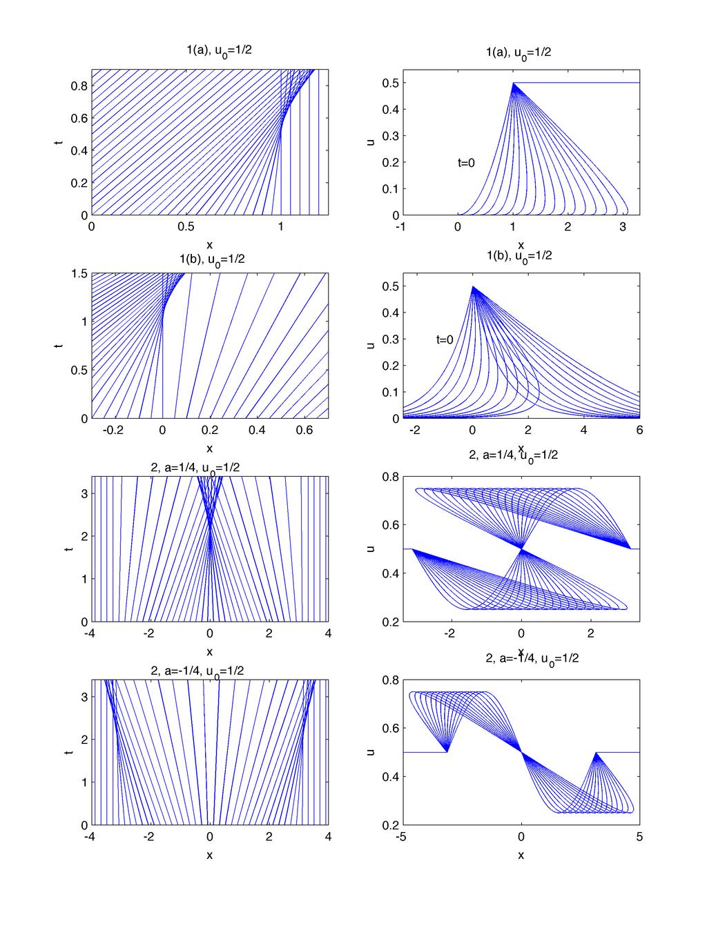
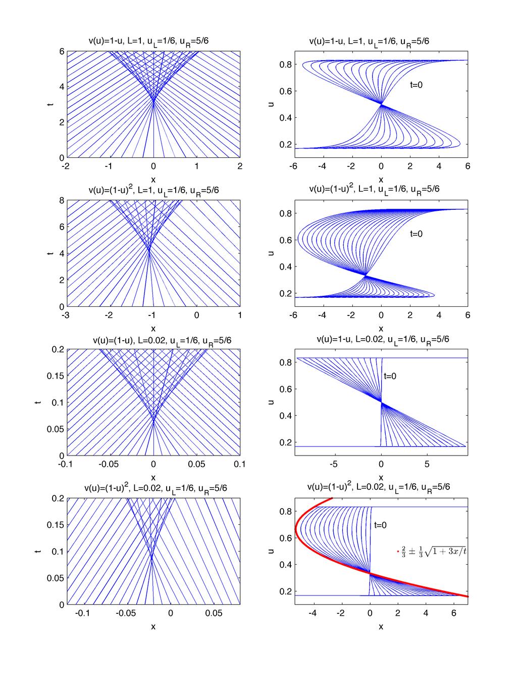
1 The flow of cars is modelled by the PDE Traffic flow problems u t + [uvu)] x = 1. If vu) = 1 u and x < a) ux, ) = u x 2 x 1 u x > 1 b) ux, ) = u e x, where < u < 1, determine when and where a shock first forms. Sketch a characteristics diagram and the solution up to the development of the shock. Use the equal areas rule to make sketches of the progress of the shock after it forms for each case. 2. Solve the PDE again for vu) = 1 u and ux, ) = u + Hπ x )a sin x with a < u, a + u < 1 and Hx) the step function. Show that when a > a single shock forms and if a <, two shocks form simultaneously, at time t = 1/2 a ) in both cases). Where do these shocks form? By fitting shocks to the multi-valued functions in each case, show that, for t 1, the maximum value of u is approximately u + π a and u + 2t t for a > and a <, respectively. Helpful comments: We have x = x 1 2u)t. For a >, u + + u = 2u and so Ẋ = 1 2u, giving Xt) = 1 2u )t. For large t, the maximum value of u also occurs at the right side of the shock, and points there came from close to x = π. Hence π 1 2u )t 1 2u)t. For a < and t 1, the maximum value of u comes from x and x < Now consider vu) = 1 u) 2. Show that cu) in u t + cu x = vanishes for u = 1 3 and has a minimum at u = 2 3. If ux, ) = u L + u R e x/l 1 + e x/l with < u R < 1 3 and 2 3 < u L < 1. Sketch the initial condition and the development of the solution for t >. How does the solution differ from the solution with v = 1 u? By consider the limit L, show that the car density changes discontinuously from u L to u L at a shock which propagates at speed c1 1 2 u L). Some helpful results: The characteristics solution implies u = fx ) and x = x tcu) if ux, ) = fx) denotes the initial condition. For v = 1 u) 2, we have cu) = d du [u1 u)2 ] = 1 u)1 3u) When L, fx) u L + u R u L )Hx), and the solution for u that bridges between u L and u R all originates from near x =. Thus, cu) = x/t or u = 2 3 ± x t. The shock speed is dx/dt = [u + 1 u + ) 2 u 1 u ) 2 ]/u + u ) = 1 + u + + u ) 2 u + u 2u + + u ). 1

2 2

3 3

4 MATH 4 Sample Final exam problems The rules for the actual exam: Closed book exam; no calculators. Answer as much as you can; credit awarded for the best three answers. Adequately explain the steps you take. e.g. if you use an expansion formula, say in one sentence why this is possible; if you quote a special function solution to an ODE, say why this is the correct one. Be as explicit as possible in giving your solutions. 1. Using separation of variables, solve the wave equation, 1 r 2 r 2 u ) 1 + r r r 2 sin θ u ) sin θ θ θ inside the unit sphere, r 1, with the boundary condition, and initial condition, u = on r = 1, = u tt, u t r, θ, ) = ur, θ, ) = 5 cos 3 θ 3 cos θ)gr). Hint: for the radial part of the problem, the substitution Rr) = Xr)/ r, may prove useful, if one sets ur, θ, t) = Rr)Y θ)t t). 1*. Solve Laplace s equation, 1 r 2 r 2 u r r ) + 1 r 2 sin θ sin θ u ) + θ θ outside the unit sphere, r 1, with the boundary condition, u1, θ, φ) = cos 3θ. 1 2 u r 2 sin 2 θ φ 2 =, 1**. Solve the heat equation, 1 r 2 r r 2 u r ) + 1 r 2 sin θ inside the unit sphere, r 1, with the boundary condition, and initial condition, u = on r = 1, sin θ u ) = u t, θ θ ur, θ, ) = 3 cos 2 θ 1)gr). Hint: for the radial part of the problem, the substitution Rr) = Xr)/ r, may prove useful. 2. Establish that F 1 {e a k } = a πa 2 + x 2 ) and f g = F 1 { ˆfĝ}, where F{f} = ˆfk), F{g} = ĝk) and f g is a convolution. Using the Fourier transform, solve the PDE, u xx + u yy =, < x <, y <, ux, ) = gx), u as y, x, 4

5 expressing your solution in terms of a single integral. 2*. Establish the convolution property of the Fourier transform, fz)gx z)dz = F 1 { ˆfk)ĝk)}. Solve the heat equation, u t = u xx, on the infinite line subject to the initial condition, ux, ) = fx), expressing your answer as the convolution integral ux, t) = fz)gx z, t)dz, where you should determine Gx, t). The region x < a of an infinite solid is initially at the uniform temperature T, the remainder being at zero temperature. By using the solution above, find the temperature at later times in terms of the error function, Erfx) = 2 x e z2 dz. π 2**. Using the Fourier transform, solve the elastic wave equation, u tt + u xxxx =, < x <, ux, ) = δx), u t x, ) =, showing that Note that ux, t) = 1 x 2 cos 4πt 4t π ). 4 cos x 2 dx = sin x 2 dx = π Establish the shift relation, L{ft a)ht a)} = e as fs) for the Laplace transform, where fs) = L{ft)}. An age-structured model of a population is based on the PDE, u t + u a = µa)u, a, t <, where ua, t) dictates the number of individuals with age a at time t; the death rate µa) is a prescribed function, and initially, ua, ) =. For age a =, the birth function is u, t) = bt) + Ba)ua, t)da, where bt) is a prescribed creation function, and Ba) is a prescribed reproductivity. Using the Laplace transform in time, show that ua, t) = Sa)L 1 { bs)e sa Ds) }, Ds) = 1 Ba)Sa)e sa da, 5

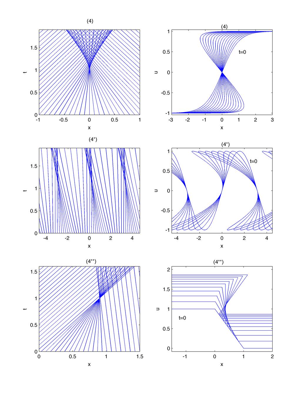
6 where the survival function, Find an explicit solution if B =. [ Sa) = exp a µa )da ]. 3*. Show that L{e at } = s a) 1, L{t n } = n!/s n+1 and L{ft a)ht a)} = e as fs). Use the Laplace transform to solve the PDE, u t + u x = u + t 2, u, t) = ft), ux, ) = 1, x < t <. 3**. Establish the relations, L{ft a)ht a)} = e as fs) and L{e bt } = b + s) 1, for the Laplace transform, where fs) = L{ft)}. The number of lightbulbs generated in a manufacturing process is given by the PDE, where µ is a constant, u t + u a = µu, a, t <, ua, ) = and u, t) = 1 + Ra)ua, t)da, with Ra) a prescribed weighting for production adjustment based on the current bulb population. Using the Laplace transform in time, show that { } e ua, t) = e µa L 1 sa, Ds) = 1 Ra)e sa µa da. sds) Find an explicit solution if R is constant, paying attention to the two cases µ R and µ = R. 4. Find an implicit algebraic formula for the solution to u t uu x =, ux, ) = tanh x. Sketch the characteristic curves on a space-time diagram and show that a shock forms at t, x) = 1, ). Write this conservation law in integral form and derive a formula determining the speed of any shocks. By arguing that u x, t) = ux, t) for x, determine what happens to the shock formed in the initial-value problem above for t > 1. 4*. For u t u 2 u x =, ux, ) = sin x. show that an infinite number of shocks form at t = 1 and find their positions. Draw the characteristic curves on a space-time diagram. 4**. Using the method of characteristics, solve u t + u 1)u x = e t, with ux, ) = 1 for x <, ux, ) = 1 x for x 1, and ux, ) = for x > 1. Sketch the characteristic curves on a space-time diagram. Show that a shock forms at t = 1; at what position does the shock first appear? 6

7 MATH 4 Final exam 217 Closed book exam; no calculators. Answer as much as you can; credit awarded for the best three answers. Adequately explain the steps you take. e.g. if you use an expansion formula, say in one sentence why this is possible; if you quote a special function solution to an ODE, say why this is the correct one. Be as explicit as possible in giving your solutions. 1. Using separation of variables, solve the wave equation, 1 r 2 r 2 u ) 1 + r r r 2 sin θ u ) sin θ θ θ inside the unit sphere, r 1, with the boundary condition, and initial condition, ur, θ, ) = u = on r = 1, = u tt, u t r, θ, ) = cos 3 θ gr). Hint: for the radial part of the problem, the substitution Rr) = Xr)/ r, may prove useful, if one sets ur, θ, t) = Rr)Y θ)t t). 2. Establish that f g = F 1 { ˆfĝ}, F 1 { ˆfak)} = 1 a fx/a) and F 1 {e k } = where F{f} = ˆfk), F{g} = ĝk), f g is a convolution, and a >. Using the Fourier transform, solve the PDE, 1 π1 + x 2 ) 4u xx + u yy =, < x <, y <, ux, ) = gx), u as y, x, expressing your solution in terms of a single integral. Give the result explicitly if g = 1 for x 1 and g = for x > Establish the relations, L{ft a)ht a)} = e as fs) and L{e bt } = b + s) 1, for the Laplace transform, where fs) = L{ft)}. An age-structured model of a population is based on the PDE, u t + u a = µa)u, a, t <, where ua, t) dictates the number of individuals with age a at time t; the death rate µa) is a prescribed function, and initially, ua, ) =. For age a =, the birth function is u, t) = bt) + Ba)ua, t)da, where bt) is a prescribed creation function, and Ba) is a prescribed reproductivity. Using the Laplace transform in time, show that { } bs)e ua, t) = Sa)L 1 sa, Ds) = 1 Ba)Sa)e sa da, Ds) 7

8 where the survival function, [ Sa) = exp a µa )da ]. Find an explicit solution for a population for which Ba) = e a, µ =, bt) = e νt and ν is a constant. 4. For u t uu x =, ux, ) = cos x. show that an infinite number of shocks form after sufficient time; determine that time and find the shock positions. Draw the characteristic curves on a space-time diagram. Sketch the solution for u upto and beyond the formation of the shock, indicating how can avoid a multivalued solution using an equal-areas rule. Briefly justify that rule using the integral form of the conservation law corresponding to the PDE and derive a formula for the speed of a shock. For the given initial condition, do the shocks move left, right or stay where they are? Helpful information: The Sturm-Liouville differential equation: [ d px) dy ] + qx)y + λσx)y =. dx dx Legendre s equation is 1 x 2 )y 2xy + nn + 1)y =. Bessel s equation is z 2 y + zy + z 2 m 2 )y =, and has the solution, y = J m z), which is regular at z =. Fourier Transforms: ˆfk) = F{fx)} = Laplace Transform: Convolution: Helpful trigonometric relations: fx)e ikx dx, fx) = F 1 { ˆfk)} = 1 2π fs) = L{ft)} = f g = ft)e st dt. fx )gx x )dx. ˆfk)e ikx dk cosa + B) = cos A cos B sin A sin B, sina + B) = sin A cos B + cos A sin B. 8

9 1. Solved in class. Some solutions 1*. If x = cos θ, then cos 3θ = 4x 3 3x = 8 5 P 3x) 3 5 P 1x), using a trig relation and given that P 1 x) = x and P 3 x) is an odd polynomial of degree 3 with normalization P n 1) = 1 so setting P 3 = Ax A)x and plugging into Legendre s equation gives A = 5 2 ). The boundary condition is independent of φ and so u = Rr)Y x). The usual separation of variables procedure implies that Rr) is given by r n 1 and Y x) by P n x) where n =, 1,... discarding the other solutions which are irregular for r and x = ±1). Hence u = n= c nr n 1 P n x) = 8 5 r 4 P 3 x) 3 5 r 2 P 1 x), given the boundary condition at r = 1. 2**. Fourier transforming the PDE and initial conditions implies û tt = k 4 û, ûk, ) = 1 and û t k, ) =. Hence ûk, t) = cos k 2 t. Inverting the Fourier transform gives ux, t) = 1 2π cos k 2 t e ikx dk = 1 4π [cosk 2 t+kx)+i sink 2 t+kx)+cosk 2 t kx) i sink 2 t kx)]dk. Using the handy changes of variable κ = tk ± x 2t ) and the trig relations again, one obtains the desired answer given integrals provided. 3*. Laplace transforming the PDE and boundary condition: ū x +s 1)ū = 1+ 2 s 3 & ū, s) = fs), ū = s3 + 2 s 3 s 1) [1 e s 1)x ]+e s 1)x fs). Inverting the Laplace transform after using a partial fraction and the shifting theorem gives u = e x ft x)ht x) + 3e t 2 2t t 2 e x [3e t x 2 2t x) t x) 2 ]Ht x). 3**. Solved in class. 4. Applying the method of characteristics gives the implicit solution u = tanh x = tanhx + ut). Hence sech 2 x u x = 1 t sech 2. x This first diverges for t = 1 at x = x =. Returning to the integral form of the conservation law, one finds that a shock located at x = Xt) travels with speed dx dt = 1 2 u+ + u ) where u ± denote the values of u to either side of the shock. Since ux, t) is odd, u = u + and so the shock is stationary. 4**. The characteristic equations are dx dt = u 1 & du dt = e t. Hence, u = fx ) + 1 e t and x = x + tfx ) + e t 1, if ux, ) = fx) denotes the initial condition. That is, u = 2 e t for x = x t e t + 1 <, u = 1 e t for x = x e t + 1 > 1 and u = 1 x t + te t 1 t for x 1 or t + e t 1 x e t. The central region shrinks to the point x = e 1 at t = 1, implying where and when the shock forms. 9

10 1

11 MATH 4, final 217 Solution points) Let u = Rr)Y x)t t) where x = cos θ. Then, separating variables, T + ω 2 T =, [1 x 2 )Y ] + λy =, r 2 R ) λr + ω 2 r 2 R =. Thus, T is given by sin ωt and Y by P n x), with λ = nn + 1) and n =, 1, 2,..., in view of ur, θ, ) = and demanding regularity at x = ±1. Introducing R = X/ r as suggested reduces the R equation to Bessel s equation with m 2 = nn + 1) n )2 and X = J m ωr), after demanding regularity at r = which eliminates Y m r). But u1, θ, t) =, and so ω must be a zero of J m z). Denoting the j th zero of J m z) by z mj, we therefore find a general solution, u = r 1/2 j=1 n= c nj sinz mj t)p n x)j m z mj r) 7 points so far, including comments as to why one chooses P n x) and J m r)/ r). The coefficients c nj must be chosed to fit the initial condition: u t r, θ, ) = x 3 gr) 1 5 [2P 3x) + 3P 1 x)]gr), given that P 1 x) = x, P n 1) = 1 and P 3 x) is an odd cubic polynomial so a little algebra with Legendre s equation gives P 3 = 5x 3 3x)/2) 2 points, some indication needed for where the polynomials come from). Hence, given the Sturm-Liouville form of Bessel s equation, c nj = 1 gr)j mz mj r)r 3/2 { dr 3/5 n = 1 1 z mj [J mz mj r)] 2 rdr 2/5 n = 3, and c nj = otherwise 2 points, some indication needed for where the weight functions come from) points) From the definition of the Fourier transform, and F{f g} = F 1 { ˆfak)} = 1 2π e ikx gx x )fx )dxdx = F 1 {e k } = 1 e ikx+k dk + 1 2π 2π which establish the desired results 3 points). Transforming the PDE: e ikz ikx gz)fx )dxdz e ikx 1 ˆfak)dk = e iκx/a) ˆfκ)dκ 2πa e ikx k dk = 1 2πix + 1) 1 2πix 1), û yy = 4k 2 û ûk, y) = ûk, )e 2 k y = ĝk)e 2 k y. Using the results above with a y and ˆf = e k gives u = 2y π = 1 π tan 1 1 x 2y gx )dx 4y 2 + x x ) 2 ) x π tan 1 2y 11 )

12 for the specific example of gx) 6 points) points) From the definitions, L{ft a)ht a)} = a L{e bt } = ft a)e st dt = e sa fτ)e sτ dτ = e sa fs) a e s+b)t dt = 1 b + s 2 points). Given L{u t a, t)} = s u)a, s) ua, ) and ua, ) =, Laplace transforming the PDE gives ū a = s + µ)ū ūa, s) = ū, s)e sa Sa). 2 points, including explicit incorporation of the initial condition and care with the limits of the integrals). Taking the transform of the condition at a = : ū, s) = bs) + which gives the desired result. 3 points). For the sample functions, Ba)ūa, s)da ū, s) = bs) Ds) & ūa, s) = Sa) bs)e sa, Ds) Sa) = 1, Ds) = s s + 1, bs) = 1 ν + s, and so ūa, s) = [ s + 1) 1 ss + ν) e sa = s 1 ν ] e sa s + ν ν & ua, t) = 1 ν Ht a)[1 1 ν)e νt a) ]. if ν, and ua, t) = 1 + t a)ht a) if ν =. 3 points, including explicit consideration of the case ν = ). Hence, points) The characteristics equations and solution: dx dt = u & du dt = x = x ut & u = cos x = cosx + ut). u x = sin x 1 + t sin x, which first diverges for x = x = 1 2 π = 3 2 π = 7 2π =... at t = 1. 3 points). The integral form of the conservation law is d dt b a ux, t)dx = 1 2 [u2 x, t)] b a For the equal-areas rule, one surgically removes the multivalued part of the solution by introducing a vertical line that cuts out equal area to either side; this is justified by the integral form of the conservation law which demands that udx the signed area underneath the curve of u) is 12

13 constant in time if there is no flux into or out of the full spatial domain a, b ). If u jumps from u to u + at x = Xt), then d X ux, t)dx + d dt a dt b X ux, t)dx = X a u t x, t)dx + Taking the limits a X and b X + now gives b X dx dt = 1 2 u+ + u ). u t x, t)dx + u + u ) dx dt = 1 2 [u2 x, t)] b a For the case at hand, the symmetry of the solution using the method of characteristics implies that u = u + and so the shocks are stationary, as also implied by the graphical solution. 5 points). Sketches: 3 points. 13