The official electronic file of this thesis or dissertation is maintained by the University Libraries on behalf of The Graduate School at Stony Brook

Transcription

1 Stony Brook University The official electronic file of this thesis or dissertation is maintained by the University Libraries on behalf of The Graduate School at Stony Brook University. Alll Rigghht tss Reesseerrvveedd bbyy Auut thhoorr..

2 Renormalization and Non-Rigidity A Dissertation Presented by Vasu Venkata Mohana Sarma Chandramouli to The Graduate School in Partial Fulfillment of the Requirements for the Degree of Doctor of Philosophy in Mathematics Stony Brook University December 2008

3 Stony Brook University The Graduate School Vasu Venkata Mohana Sarma Chandramouli We, the dissertation committee for the above candidate for the Doctor of Philosophy degree, hereby recommend acceptance of this dissertation. Marco Martens Associate Professor, Dept. of Mathematics, Stony Brook University, USA Dissertation Advisor Wim Nieuwpoort Professor Emeritus, Dept. of Chemistry, RuG Groningen, The Netherlands Chairman of Dissertation Henk Broer Professor, Dept. of Mathematics, RuG Groningen, The Netherlands Scott Sutherland Associate Professor, Dept. of Mathematics, Stony Brook University, USA Jeremy Kahn Lecturer, Dept. of Mathematics, Stony Brook University, USA Roland Roeder Post-doctoral Fellow, Dept. of Mathematics, Stony Brook University, USA Michael Benedicks Professor, Dept. of Mathematics, KTH Stockholm, Sweden Outside Member André de Carvalho Assistant Professor, Dept. of Mathematics, USP Sao Paulo, Brazil Outside Member Sebastian van Strien Professor, Dept. of Mathematics, University of Warwick, United Kingdom Outside Member This dissertation is accepted by the Graduate School Lawrence Martin Dean of the Graduate School ii

4 Agreement of Joint Program The following is a dissertation submitted in partial fulfillment of the requirements for the degree Doctor of Philosophy in Mathematics awarded jointly by Rijksuniversiteit Groningen, The Netherlands and Stony Brook University, USA. It has been agreed that neither institution shall award a full doctorate. It has been agreed by both institutions that the following are to be the advisors and reading committee. Advisors: Prof. H.W. Broer, Rijksuniversiteit Groningen Assoc. Prof. M. Martens, Stony Brook University Reading Committee: Prof. M. Benedicks, KTH Stockholm, Sweden Prof. S. van Strien, University of Warwick, UK Ass. Prof. A. de Carvalho, USP Sao Paulo, Brazil Assoc. Prof. S. Sutherland, Stony Brook University Dr. J. Kahn, Stony Brook University Dr. R. Roeder, Stony Brook University Chair of the Defense: Prof. W.C. Nieuwpoort, Rijksuniversiteit Groningen Both institutions agree that the defense of the above degree will take place on Monday 8th December 2008 at 3:00pm at the Academiegebouw, Rijksuniversiteit, Groningen, The Netherlands and that, if successful, the degree Doctor of Philosophy in Mathematics will be awarded jointly by Rector Magnificus, dr. F. Zwarts, RuG, Groningen, and Prof. L. Martin, Graduate School Dean, Stony Brook University. I hereby agree that I shall always describe the diplomas from Stony Brook University and Rijksuniversiteit Groningen as representing the same doctorate. V V M Sarma Chandramouli iii

5 Abstract of the Dissertation Renormalization and Non-Rigidity by Vasu Venkata Mohana Sarma Chandramouli Doctor of Philosophy in Mathematics Stony Brook University 2008 The aim of the thesis is to study the renormalization of unimodal maps with low smoothness and the dynamics of Hénon renormalization. M. Feigenbaum and by P. Coullet and C. Tresser in the nineteen-seventieth to study the asymptotic small scale geometry of the attractor of one-dimensional systems which are at the transition from simple to chaotic dynamics. This geometry turns out to not depend on the choice of the map under rather mild smoothness conditions. The existence of a unique renormalization fixed point which is also hyperbolic among generic smooth enough maps plays a crucial role in the corresponding renormalization theory. The uniqueness and hyperbolicity of the renormalization fixed point were first shown in the holomorphic context, by means that generalize to other renormalization operators. It was then proved that in the space of C 2+α unimodal maps, for α > 0, the period doubling renormalization fixed point is hyperbolic as well. In this thesis work we study what happens when one approaches from below the minimal smoothness thresholds for the uniqueness and for the hyperbolicity of the period doubling renormalization generic fixed point. Indeed, our main result states that in the space of C 2 unimodal maps the analytic fixed point is not hyperbolic and that the same remains true when adding enough smoothness to get a priori bounds. In this smoother class, called C 2+, the failure of hyperbolicity is tamer than in C 2. Things get much worse with just a bit less of smoothness than C 2 as then even the uniqueness is lost and other asymptotic behavior become possible. Furthermore, we show that the period doubling renormalization operator acting on the space of C 1+Lip unimodal maps has infinite topological entropy. The second part of the thesis work is devoted to the renormalization of Hénon maps. It was shown that for strongly dissipative Hénon maps, there is a short curve in the parameter space which consists of infinitely renormalizable Hénon maps of period doubling type. In this thesis we study numerically, the extension of this curve in the parameter space up to the conservative map. More precisely, we describe the combinatorial changes which occur along this curve. The second part of this study is to describe, how the one-dimensional Cantor set deforms into the Cantor set of conservative map. To show this we compute the distribution of angles of the line fields along the Cantor set and explain how this geometry becomes more complicated for maps close to the infinitely renormalizable conservative maps. iv

6 To my parents and Guruji

7 Contents List of Figures Acknowledgements viii xi 1 Introduction 1 2 Chaotic Period Doubling Introduction Notation Renormalization of C 1+Lip unimodal maps Piece-wise affine infinitely renormalizable maps C 1+Lip extension Entropy of renormalization Chaotic scaling data Renormalization of C 2 unimodal maps C 2+ unimodal maps Distortion of cross ratios A priori bounds Approximation of f I n j by a quadratic map Approximation of R n f by a polynomial map Convergence Slow convergence Hénon Renormalization Introduction Notation Hénon cycles Construction of the period 2 n points Construction of period k points with Fibonacci combinatorics Flow of periodic orbits Break-up process of Hénon renormalization Line fields on the Cantor set vi

8 4.7 Distributional Universality Summary 89 Bibliography 92 vii

9 List of Figures 1.1 Left: distribution of angles for b = 0.0; Right: for b = {c} = n 1 I0 n The graph of f σ I n Next generation of intervals around the critical interval R n f σ The graphs of A 0,A 1 and A 0 + A R : C R Extension of f σ ǫ variation of f σ Horseshoe Illustration of the next generation intervals of I0 n and În Chaotic extension most attracting curve Γ 2 n in the (a,b) parameter plane the parameter curves Γ 2 n for n < Fibonacci parameter curves of periods 2 and Fibonacci parameter curves of periods 5 and Fibonacci parameter curves of periods 13 and The sequence of good parameter curves 2, 5, 13, 34, Top: period 5, 13 and 34; Bottom: Magnification of period 13 and projection of periodic orbit of periods 2 5 and projection of periodic orbit 2 7 and crossing of periodic flow of period projection of periodic orbit 5 and 13 with Fibonacci combinatorics projection of periodic orbit 34 with Fibonacci combinatorics A renormalizable Hénon-like map Left:first bifurcation moment at b 1 on Γ 2 n;right:magnification around the point, where the unstable manifold touches the stable manifold Non 2 renormalizable Hénon-like map the curve Γ 2 n viii

10 4.17 first heteroclinic tangency at b 1 ; β 0,β 1 are fixed points; W u (β 0 ) is the unstable manifold of β 0 and W s (β 1 ) is the stable manifold of β second heteroclinic tangency at b 2 ; β 1 is a fixed point and β 2 is period 2 point; W u (β 1 ) is the unstable manifold of β 1 and W s (β 2 ) is the stable manifold of β Left: Third heteroclinic tangency at b 3 ; β 2 is period 2 point and β 3 is period 4 point; W u (β 2 ) is unstable manifold of β 2 and W s (β 3 ) is the stable manifold of β 3 ; Right: Magnification of the box in Figure(a) Left: Fourth heteroclinic tangency at b 4 ; β 4 is period 8 point and β 5 is period 16 point; W u (β 4 ) is the unstable manifold of β 4 and W s (β 5 ) is the stable manifold of β 5 ; Right: Magnification of the box in Figure (a) Left: Fifth heteroclinic tangency at b 5 ; β 5 is period 2 4 point and β 4 is period 2 3 point; W u (β 5 ) is unstable manifold of β 5 and W s (β 4 ) is the stable manifold of β 4 ; Right: Magnification of the box in Figure (a( Left: Sixth heteroclinic tangency at b 6 ; β 6 is period 2 5 point and β 5 is period 2 4 point; W u (β 6 ) is the unstable manifold of β 6 and W s (β 5 ) is the stable manifold of β 5 ; Right: Magnification of the box in Figure (a) Left: Seventh heteroclinic tangency at b 7 ; β 7 is period 2 6 point and β 6 is period 2 5 point; W u (β 7 ) is unstable manifold of β 7 and W s (β 6 ) is the stable manifold of β 6 ; Right: Magnification of the box in Figure (a) Left: Eighth heteroclinic tangency at b 8 ; β 8 is period 2 7 point and β 7 is period 2 6 point; W u (β 8 ) is the unstable manifold of β 8 and W s (β 7 ) is the stable manifold of β 7 ; Right: Magnification of the box in Figure (a) distribution of the angles of line fields for b = 0; and b = distribution of the angles of line fields for b = 0.2 and b = distribution of the angles of line fields for b = 0.4 and b = distribution of the angles of the line fields for b = 0.6 and b = distribution of angles of the line fields for b = 0.8 and b = Top: distribution of angles for the degenerate map; Below: for the map b = time versus angle for b = 0.0 to b = time versus angle for b = 0.4 to b = time versus angle for b = 0.8 and b = comparison of angles; Top:b = 0.0; Below: b = Left: line fields for b = 0.0; Right: b = Left: line fields for b = 0.2; Right: b = Left: line fields for b = 0.4; Right: b = Left: line fields for b = 0.6; Right: b = Left: line fields for b = 0.8; Right: b = ix

11 4.40 b versus average for downward angles on the curve Γ 2 11; n. lev indicates the nth zoom level around the point β n b versus average for downward angles on the curve Γ 2 13; n lev indicates the nth zoom level around the point β n b versus average for downward angles on the curve Γ 2 11; n lev indicates the nth zoom level around the point l p b versus average for downward angles on the curve Γ 2 13; n lev indicates the nth zoom level around the point l p b versus average for downward angles; periodic orbit of period 2 13 ; 11. lev indicates the zoom level at the point l p b versus average for upward angle; periodic orbit of period 2 13 ; 11. lev indicates the zoom level at the point l p x

12 Acknowledgements I would like to take this opportunity to express my gratitude to everyone who have helped me during the completion of this thesis work. First of all, I would like to thank my advisor Dr. Marco Martens for his inspiring guidance, invaluable suggestions and constant encouragement throughout the last four years. I am grateful to him. Many thanks to Peter Hazard. We both started research work at the same time in RuG and came to stony brook together for completing the rest of the thesis work. During the span of last four years he has been a good friend. I thank him for several useful mathematical discussions and for proof-reading of the chapter 4 of this work. I am thankful to the members of the reading committee, Prof. M. Benedicks, Prof. S. van Strien and Prof. A. de Carvalho for their willingness to read and evaluate the thesis. With great pleasure, I thank Dr. Charles Tresser and Prof. Welington de Melo, who are the co-authors of the publication that is the part of this work. The collaboration with them has provided important insights on many questions in the first part of this thesis. I also thank Björn Winkcler, Olga Lukina, Stephen Meagher, Lenny Taelmann, Sijbo Holtman, Khairul Saleh, Mark opmeer, Ricardo Zavala Yó, Diego Napp and Easwara Subramanian for many discussions that I had with them. Special thanks to my Art of Living friends, Francesca, Maja, and Miguel. I had a good time with them. I still remember the beginning days in Groningen and many warm memories which i had with Ravi, Pramod, Ansar and other members of GISA. I thank everyone. I owe my appreciation to Marco Martens and Lucienne Pereira for their hospitality and kind help in many situations. The remaining acknowledgement comes from the period I have spent in Stony Brook. I would like to thank Prof. J. Milnor for suggesting the numerical problem on Hénon maps and it was reflected as chapter 4, with many interesting directions. I learned a lot from the courses given by Prof. M. Lyubich and also from the Dynamics seminar. I would like to thank all the people in the Dynamics group at stony brook for their help. Many thanks goes to the other grad students, especially in the 2nd floor of Math Tower for creating a pleasant working place and for being very helpful.

13 Finally, I thank all the staff members at both RuG and Stony Brook for their help during the time of this dissertation work, in particular Esmee Elshof, Desiree Hansen, Ineke Schelhaas, Helga Steenhuis, Annette Korringa, Yvonne van der Weerd, Elizabeth Woldringh for taking care of the administrative issues and Peter Arendz, Harm Paas, Jurjen Bokma for their system support. Special thanks goes to Kees Visser for providing an access to the Opteron Cluster and his support during the time of my computational work. At Stony Brook, I thank, Donna McWilliams, Nancy Rohring, Gerri Sciulli and Patrick Tonra. I must thank Prof. H.W. Broer for all the arrangements he made for the defense during the last six months and also Prof. M. Anderson and Prof. C. LeBrun at Stony Brook. Last but not least, I am indebted to my parents for their love, patience and understanding. Thanks to Padmaakka, Siva Rama Krishna Bava, Bhanuakka, Subbarao Bava, Satyanarayana Mavayya, Jaya Attayya, Hanuma vadina and Murali annayya. Without their support I would have not come to abroad and do the research. I am very much grateful to them for the love and affection they have towards me.

14 Chapter 1 Introduction The study of time evolution of the systems under consideration plays an important role in many natural sciences. Experiments and simulations in these fields often show very complicated, chaotic behavior. However, a rigorous understanding of chaotic dynamical systems are far from complete. There are not many real world systems which can be modeled by one dimensional dynamical systems. That is, systems described by iteration of a map of the interval. Nevertheless, during the last forty years an extensive and rather complete theory has been developed to explain their dynamics. The surprising fact is that many of the one dimensional phenomena are observed in nature. Although one dimensional systems are very simple models, they contain mechanisms which are relevant for real world systems. The natural strategy is to explore, how far we can extend the one dimensional theory and get a better understanding of higher dimensional systems. The central theme of the one-dimensional theory is the geometric rigidity of the attractors. The main technique is renormalization. Renormalization is a method to study the microscopic geometric properties of attractors. It was introduced into dynamics in the late seventies by P. Coullet and C.P. Tresser [7] and independently M.J. Feigenbaum [14]. Initially the goal was to study the dynamics at the accumulation of period doubling. Systems which are at the accumulation of period doubling have very specific combinatorial behavior. This behavior occurs when a system is at transition to chaos, when it is at the boundary of chaos in the space of systems. The attractors of the maps at transition to chaos have a special property. They are Cantor sets and on arbitrarily small scale the attractor can be identified with a rescaled version of the attractor of another one-dimensional map. This allows to introduce an operator on the set of one-dimensional maps at transition which assigns to a map, the map which describes its attractor at the smaller scale. This operator acts as a microscope. For maps at the transition we can describe the dynamics at arbitrarily small scale. That is, we can apply the renormalization operator infinitely many times to study the dynamics. It was conjectured in [7] and [14], that the maps at transition form exactly the 1

15 stable manifold of a unique fixed point f of the renormalization operator. This conjecture explains why the fine scale structure of the attractor is independent of the original map being considered. The microscopic geometry of an attractor at transition to chaos is universal. The fine scale geometrical structure can not be deformed. The attractors are rigid. During the following thirty years the renormalization idea was extended and applied to general types of combinatorics of one-dimensional maps. Our understanding of one-dimensional dynamics is a consequence of the maturity of one-dimensional renormalization. A general theory for smooth dynamics is still completely out of reach. There are two natural directions in which one can extend the theory using the results from one-dimensional smooth dynamics. The first one is one-dimensional dynamics with low smoothness and the second is dynamics of Hénon maps. Models of real world systems are usually very high dimensional or even infinite dimensional as in fluid dynamics. However, there is a phenomenon of dimension reduction, the essence of the dynamics happens on low dimensional attractors. On some cases these attractors can be described, even in terms of one-dimensional systems. This is the reason why one-dimensional dynamical systems are more than just toy models. The theory for one-dimensional systems is well developed in the case, when the systems are smooth. Unfortunately, the one-dimensional systems which arise from applications are usually not smooth. In dissipative systems the states are groups in so-called stable manifolds, different states in such a stable manifold have the same future. The packing of the stable manifold usually does not occur in a smooth way. For example, the Lorenz flow is a flow on three dimensional space approximating a convection problem in fluid dynamics. The stable manifolds are two dimensional surfaces packed in a non smooth foliation. This flow can be understood by a map on the interval whose smoothness is usually below C 2. The first part of the thesis discusses renormalization of one-dimensional maps with low smoothness. The first group of results deals with the maps which are C 2. All maps under consideration will be the maps with a quadratic tip. These maps are unimodal, they have a single maximum at their critical point, it is denoted by c and this maximum is well approximated by a quadratic polynomial. The collection of unimodal maps with quadratic tip and a certain smoothness is denoted by U r. The main results lead to the fact that renormalization on the space of C 2 unimodal maps is not hyperbolic and the convergence to the analytic fixed point can be arbitrarily slow. Theorem Let d n > 0 be any sequence with d n 0. There exists an infinitely renormalizable C 2 unimodal map f U 2 such that dist 0 (R n f,f ω ) d n. The distance is measured in the C 0 topology. 2

16 Corollary The analytic unimodal map f ω is not a hyperbolic fixed point in the space of C 2 unimodal maps. We introduce a new type of differentiability of a unimodal map, called C 2+, which is the minimal needed to be able to apply the classical proofs of a priori bounds for the invariant Cantor sets of infinitely renormalizable maps, see for example [24],[26],[11]. This type of differentiability will allow us to represent any C 2+ unimodal map as f = φ q, where q is a quadratic polynomial and φ has still enough differentiability to control cross-ratio distortion. Theorem If f is an infinitely renormalizable C 2+ unimodal map then lim dist 0 (R n f, f ω ) = 0. n A construction similar to the one provided for C 2 unimodal maps leads to the following result: Theorem Let d n > 0 be any sequence with n 1 d n <. There exists an infinitely renormalizable C 2+ unimodal map f such that dist 0 (R n f,f ω ) d n. The analytic unimodal map f ω of C 2+ maps. is not a hyperbolic fixed point in the space of Our second set of theorems deals with renormalization of C 1+Lip unimodal maps with a quadratic tip. Theorem There exists an infinitely renormalizable C 1+Lip unimodal map f which is not C 2 but Rf = f. The topological entropy of a system defined on a non-compact space is defined to be the Supremum of the topological entropies contained in compact invariant subsets. As a consequence of a Theorem of Davie [8], we get that renormalization on U 2+α has entropy zero, for any α > 0. Theorem The renormalization operator acting on the space of C 1+Lip unimodal maps has infinite entropy. The last theorem illustrates a specific aspect of the chaotic behavior of the renormalization operator on the space of C 1+Lip unimodal maps. Theorem There exists an infinitely renormalizable C 1+Lip unimodal map f such that {c n } n 0 is dense in a Cantor set. Here c n is the critical point of R n f. 3

17 The second possibility is to use the successful one-dimensional renormalization theory to study two-dimensional dynamics. In the case of dissipative dynamics we should start with the Hénon family. The maps in this family act on a two-dimensional domain and are given by F a,b (x,y) = (f a (x) by,x), where b 0, is the Jacobian and f a (x) is a unimodal map. This family arises when one creates chaos from a homoclinic bifurcation in a dissipative system. Strongly dissipative Hénon maps, b << 1, are perturbations of one dimensional dynamics and one-dimensional renormalization theory is a powerful starting point for the development of a theory. The Hénon family has many realistic applications because of its relevance in the creation of chaos. Rigorous understanding of Hénon map is fragmented. There are three well understood phenomena. The first one is the Newhouse phenomenon [28]. There are smooth maps (also in the Hénon family) which have periodic attractors of arbitrarily high period. This behavior is quite different form the chaotic maps constructed by M. Benedicks and L. Carleson [3]. They proved that for a set of parameters with positive measure the corresponding Hénon map has a nontrivial attractor with an ergodic invariant measure, describing the statistical long term behavior of typical orbits. This fundamental work from the late eighties was recently refined by L.S. Young and Q.D. Wang to apply higher dimensions, Hénon-like maps [33]. The third part of our knowledge of Hénon maps deals with the maps in a neighborhood of the accumulation of period doubling. This is an area in the parameter space where chaos is created. The first study of this area was done by P. Collet, J-P. Eckmann and H. Koch, [6]. They used analytical tools to extend the one-dimensional renormalization operator to a space of strongly dissipative Hénon-like maps and proved the hyperbolicity of the operator. A. de Carvalho, M.Lyubich, and M. Martens constructed a renormalization operator on the space of strongly dissipative Hénon-like maps using geometric ingredients, [9]. The specific construction and the hyperbolicity of this renormalization operator allowed to study the geometry of Cantor attractors of Hénon maps at the accumulation of period doubling. It opened a source of surprising phenomena. The results obtained, discuss the geometric (non)-rigidity of the Cantor attractors of maps at the accumulation of period doubling, the topology of such maps as well as the bifurcation pattern in a neighborhood of the accumulation of period doubling. The main theme is that the theory for two-dimensional dissipative dynamics is far from a straightforward generalization of the onedimensional theory, even for maps which are the simplest combinatorial type, period doubling. However, renormalization is again a very powerful tool which is able to describe the dynamics of Hénon maps. The second part of the thesis discusses renormalization for Hénon maps. It is a numerical study. The present renormalization theory deals with strongly dissipative Hénon maps. These maps form a short curve in parameter space of 4

18 a generic Hénon family. An important question is whether the observed phenomena of (non-)rigidity and universality can be extended to the maps which are (not strongly) dissipative and even up to the conservative maps. Briefly speaking, can we extend the curve of infinitely renormalizable strongly dissipative Hénon maps up to the conservative maps? The first numerical study shows that, indeed, the curve extend that far. More importantly, the study describes the combinatorial changes which occur along this curve. These changes are denoted by top-down breaking of the boxes. Most of the results for Hénon maps discuss strongly dissipative maps, b << 1. We do not yet have the tools to study maps which are not strongly dissipative, maps which are not small perturbations of one-dimensional maps. The numerical description of top-down breaking of boxes indicates that, how one can proceed to rigorously extend the curve up to the conservative maps. One-dimensional dynamics is controlled by the critical points of these systems. Infinitely renormalizable Hénon maps also have a topologically defined critical points which plays a crucial role. At the present moment we are at the starting point of developing a renormalization theory for Hénon maps with more general combinatorial types. Part of the problem is to describe the combinatorial type of Hénon map. History inspires us to consider Hénon-like maps of Fibonacci type. Unfortunately, the situation is far more complex than the period doubling case for Hénon maps. There are infinitely many critical points. However, a numerical study presented in this thesis shows that there is a curve in the Hénon family whose maps have an invariant Cantor set of Fibonacci type. This is a strong support for the possibility of constructing a renormalization operator for Hénon maps of Fibonacci type. Infinitely renormalizable Hénon maps of period doubling type have a Cantor attractor. This Cantor set has geometrical aspects which are exactly the same as the counter part in the Cantor attractors of infinitely renormalizable onedimensional systems. This phenomenon is called universality. Contrary to the one-dimensional situation, these Hénon Cantor sets are not rigid. There are parts of the Hénon Cantor set where the geometry on asymptotically small scale is different from the one-dimensional situation. By changing the Jacobian b one can change the asymptotic geometry of the Cantor set. The non-rigidity was up to recently an unexpected phenomenon. Strongly dissipative two-dimensional systems are geometrically different from the one-dimensional world. Although, two and one-dimensional systems do have some universal geometrical aspects. The numerically constructed curve of infinitely renormalizable dissipative Hénon maps ends at conservative map. This conservative map has an invariant Cantor set. The geometry of this Cantor set is not at all similar to the Cantor attractor of the dissipative maps. Our third numerical study on Hénon maps discusses how the one-dimensional Cantor set deforms into the Cantor set of the conservative map. To describe this deformation we studied the invariant line field which is carried on the Cantor set. This line field has zero characteristic exponent. One could think about this line field as if it was aligned along the Cantor set. However, one should be careful. It has been shown that this line 5

19 field is not continuous for truly two-dimensional Hénon maps [9]. The Cantor set does not lie on a smooth curve. We study numerically, the distribution of the angles of the lines in the line field with respect to a fixed direction. Initially, for strongly dissipative maps, the angles are distributed in a Cantor set. This is not surprising. However, if we consider infinitely renormalizable maps on the curve closer towards the end with the conservative map, the distributions are assigning weight to all angles. These distribution of angles in extreme cases, b = 0 and b = 0.95, are illustrated in Figure Figure 1.1: Left: distribution of angles for b = 0.0; Right: for b = 0.95 Observe that, these Cantor sets are always having Hausdorff dimension smaller than one. It is not filling more and more the space. The appearance of more and more angles is a result from the more and more complexity of the geometry of Cantor set. It gets more and more away from being on a smooth curve. This refined understanding might play a crucial role in further studies of Hénon maps. Simple questions like the existence of wandering domains is closely related to the geometry of the line field. The non-existence of wandering domains is still open. The short term goals of this thesis is to contribute to our understanding at the accumulation of period doubling and get a complete understanding of this type of dynamics. The second short term goal is to develop a renormalization theory which can be applied to more general types of combinatorics, beyond period doubling and study the corresponding dynamics. This will provide fundamental pieces of the larger Hénon puzzle. The long term goal is to understand two-dimensional dynamics. The conjecture which describes the behavior of smooth dynamics in general was formulated by J. Palis [29]. It is the central theme of smooth dynamics. The essence of the conjecture is as follows. Almost every map in a generic family has finitely many attractors: almost every orbit accumulates at one of them. Furthermore, each attractor carries an invariant measure which describes the statistical behavior of a typical orbit in its basin. Systems with zero entropy can be understood in purely topological terms. Namely, the Morse-Smale systems are dense among zero entropy systems. 6

20 The conjecture has a long history. In particular, it took several decades to observe that, as well topological as measure theoretical ingredients are necessary to understand smooth dynamics. The first context in which the Palis Conjecture was proved is unimodal dynamics on the interval. The main techniques used to prove the Palis Conjecture in one dimension are centered around renormalization. Indeed, the fine geometrical properties of unimodal maps are closely related to the phenomena described in the conjecture. The Palis Conjecture is the long term goal of smooth dynamics. We are still far from such a general understanding. However, it as been proved in onedimension. The next natural step is to go to two-dimensional dynamics, the Hénon family. The results by M. Benedicks and L. Carleson are the first fundamental steps towards the Palis Conjecture for Hénon maps. The renormalization work done at the accumulation of period doubling was used to show that the Morse- Smale maps are dense in the set of strongly dissipative Hénon maps with entropy zero, [22]. Although, even this result on density of Morse-Smale maps is more involved than the one-dimensional counterpart, renormalization technique is able to deal with the situation. As in one-dimension, renormalization should become an intrinsic part of a comprehensive picture of two-dimensional dynamics. 7

21 Renormalization of C 1+Lip and C 2 unimodal maps

22 Chapter 2 Chaotic Period Doubling The period doubling renormalization operator was introduced by M. Feigenbaum and by P. Coullet and C. Tresser in the nineteen-seventieth to study the asymptotic small scale geometry of the attractor of one-dimensional systems which are at the transition from simple to chaotic dynamics. This geometry turns out to not depend on the choice of the map under rather mild smoothness conditions. The existence of a unique renormalization fixed point which is also hyperbolic among generic smooth enough maps plays a crucial role in the corresponding renormalization theory. The uniqueness and hyperbolicity of the renormalization fixed point were first shown in the holomorphic context, by means that generalize to other renormalization operators. It was then proved that in the space of C 2+α unimodal maps, for α > 0, the period doubling renormalization fixed point is hyperbolic as well. In this work we study what happens when one approaches from below the minimal smoothness thresholds for the uniqueness and for the hyperbolicity of the period doubling renormalization generic fixed point. Indeed, our main results states that in the space of C 2 unimodal maps the analytic fixed point is not hyperbolic and that the same remains true when adding enough smoothness to get a priori bounds. In this smoother class, called C 2+ the failure of hyperbolicity is tamer than in C 2. Things get much worse with just a bit less of smoothness than C 2 as then even the uniqueness is lost and other asymptotic behavior become possible. We show that the period doubling renormalization operator acting on the space of C 1+Lip unimodal maps has infinite topological entropy. 2.1 Introduction The period doubling renormalization operator was introduced by M. Feigenbaum [14], [15] and by P. Coullet and C. Tresser [7], [32] to study the asymptotic small scale geometry of the attractor of one-dimensional systems which are at the transition from simple to chaotic dynamics. In 1978, they published certain rigidity properties of such systems, the small scale geometry of the invariant 9

23 Cantor set of generic smooth maps at the boundary of chaos being independent of the particular map under consideration. Coullet and Tresser treated this phenomenon as similar to universality that has been observed in critical phenomena for long and explained since the early seventieth by Kenneth Wilson (see, e.g., [23]). In an attempt to explain universality at the transition to chaos, both groups formulated the following conjectures that are similar to what was conjectured in statistical mechanics. Renormalization conjectures: In the proper class of maps, the period doubling renormalization operator has a unique fixed point that is hyperbolic with a onedimensional unstable manifold and a codimension one stable manifold consisting of the systems at the transition to chaos. These conjectures were extended to other types of dynamics on the interval and on other manifolds but we will not be concerned here with such generalizations. During the last 30 years many authors have contributed to the development of a rigorous theory proving the renormalization conjectures and explaining the phenomenology. The ultimate goal may still be far since the universality class of smooth maps at the boundary of chaos contains many sorts of dynamical systems, including useful differential models of natural phenomena and there even are predictions about natural phenomena in [7], which turned out to be experimentally corroborated. A historical review of the mathematics that have been developed can be found in [10] so that we recall here only a few milestones that will serve to better understand the contribution to the overall picture brought by the present work. The type of differentiability of the systems under consideration has a crucial influence on the actual small scale geometrical behavior (like it is the case in the related problem of smooth conjugacy of circle diffeomorphisms to rotations: compare [17, 34] to [18] and [19]). The first result dealt with holomorphic systems and were first local [20], and later global [30], [27], [21] (a progression similar to what had been seen in the problem of smooth conjugacy to rotations: compare [1] to [17] and [34]). With global methods came also means to consider other renormalizations. Indeed, the hyperbolicity of the unique renormalization fixed point has been shown in [20] for period doubling, and later in [21] by means that generalize to other sorts of dynamics. Then it was shown in [8] that the renormalization fixed point is also hyperbolic in the space of C 2+α unimodal maps with α > 0 (using [20]). These results were later extended in [10] to a more general types of renormalization (using [21]). After the results of Lanford [20], the existence of renormalization fixed points has been proved in more generality. First Epstein [13] constructed period doubling fixed points with arbitrary critical behavior. Renormalization fixed points do exist for any given combinatorics and arbitrary critical behavior, see [25]. In this study, we are interested in exploring from below the limit of smoothness that permits hyperbolicity of the fixed point of renormalization. Our main result concern a new smoothness class, C 2+, which is bigger than C 2+α for any positive α 1, and is in fact wider than C 2 in ways that are rather technical as we shall describe later (this is the bigger class, where the usual method to get 10

24 a priori bounds for the geometry of the Cantor set works). We are interested here in the part of hyperbolicity that consists in the attraction in the stable manifold made of infinitely renomalizable maps (hence the part covered in [30], [27] while the expansion along the unstable manifold comes from [21] as far as the global theory is concerned: see [20], [12] for the local picture). We show that in the space of C 2+ unimodal maps the analytic fixed point is not hyperbolic for the action of the period doubling renormalization operator. We also show that nevertheless, the renormalization converges to the analytic generic fixed point (here generic means that the second derivative at the critical point is not zero), proving it to be globally unique, a uniqueness that was formerly known in classes smaller than C 2+ (that is assuming more smoothness). The convergence might only be polynomial as a concrete sign of non-hyperbolicity. The failure of hyperbolicity happens in a more serious way in the space of C 2 unimodal maps since there the convergence can be arbitrarily slow. The uniqueness of the fixed point in this case, remains an open question. The uniqueness was known to be wrong in a serious way among C 1+Lip unimodal maps since a continuum of fixed points of renormalization could be produced [31]. Here we show that the period doubling renormalization operator acting on the space of C 1+Lip unimodal maps has infinite topological entropy. After this informal discussion of what will be done here and how it relates to universality theory, we now give some definitions, which allow us next to turn to the precise formulation of our main results. A unimodal map f : [0,1] [0,1] is a C 1 mapping with the following properties. f(1) = 0, there is a unique point c (0,1), the critical point, where Df(c) = 0, f(c) = 1. A map is a C r unimodal maps if f is C r. We will concentrate on unimodal maps of the type C 1+Lip, C 2, and C 2+. This last type of differentiability will be introduced in Section 3.1. The critical point c of a C 2 unimodal map f is called non-flat if D 2 f(c) 0. A critical point c of a unimodal map f has a quadratic tip if there exists a sequence of points x n c and constant A > 0 such that f(x n ) f(c) lim n (x n c) 2 = A. The set of C r unimodal maps with a quadratic tip is denoted by U r. We will consider different metrics on this set denoted by dist k with k = 0,1,2 (in fact the usual C k metrics). A unimodal map f : [0,1] [0,1] with quadratic tip c is renormalizable if c [f 2 (c),f 4 (c)] I 1 0, 11

25 f(i 1 0) = [f 3 (c),f(c)] I 1 1, I 1 0 I 1 1 =. The set of renormalizable C r unimodal maps is denoted by U r 0 U r. Let f U r 0 be a renormalizable map. The renormalization of f is defined by Rf(x) = h 1 f 2 h(x), where h : [0,1] I 1 0 is the orientation reversing affine homeomorphism. This map Rf is again a unimodal map. The nonlinear operator R : U r 0 U r defined by R : f Rf is called the renormalization operator. The set of infinitely renormalizable maps is denoted by W r = n 1 R n (U r 0). There are many fundamental steps needed to reach the following result by Davie, see [8]. For a brief history see [10] and references therein. Theorem (Davie) There exists α < 1 such that the following holds. In the space of U 2+α, there exists a unique renormalization fixed point f ω, with the following properties f ω is analytic, f ω is a hyperbolic fixed point of R : U 2+α 0 U 2+α, the codimension one stable manifold of f ω coincides with W 2+α, f ω has a one dimensional unstable manifold which consists of analytic maps. In our discussion we only deal with period doubling renormalization. However, there are other renormalization schemes. The hyperbolicity for the corresponding generalized renormalization operator has been established in [10]. Our main results deal with R : U r 0 U r where r {1 + Lip,2,2 + }. Theorem Let d n > 0 be any sequence with d n 0. There exists an infinitely renormalizable C 2 unimodal map f with quadratic tip such that dist 0 (R n f,f ω ) d n. Corollary The analytic unimodal map f ω of R : U0 2 U 2. is not a hyperbolic fixed point 12

26 In Section 3.1 we will introduce a type of differentiability of a unimodal map, called C 2+, which is the minimal needed to be able to apply the classical proofs of a priori bounds for the invariant Cantor sets of infinitely renormalizable maps, see for example [24],[26],[11]. This type of differentiability will allow us to represent any C 2+ unimodal map as f = φ q, where q is a quadratic polynomial and φ has still enough differentiability to control cross-ratio distortion. The precise description of this decomposition is given in Proposition For completeness we include the proof of the a priori bounds in Section 3.3. Theorem If f is an infinitely renormalizable C 2+ unimodal map then lim n dist 0 (R n f, f ω ) = 0. A construction similar to the one provided for C 2 unimodal maps leads to the following result: Theorem Let d n > 0 be any sequence with n 1 d n <. There exists an infinitely renormalizable C 2+ unimodal map f with a quadratic tip such that dist 0 (R n f,f ω ) d n. The analytic unimodal map f ω is not a hyperbolic fixed point of R : U 2+ 0 U 2+. Our second set of theorems deals with renormalization of C 1+Lip unimodal maps with a quadratic tip. Theorem There exists an infinitely renormalizable C 1+Lip unimodal map f with a quadratic tip which is not C 2 but Rf = f. The topological entropy of a system defined on a non-compact space is defined to be the Supremum of the topological entropies contained in compact invariant subsets: we will always mean topological entropy when the type of entropy is not specified. As a consequence of Theorem we get that renormalization on U 2+α 0 has entropy zero. Theorem The renormalization operator acting on the space of C 1+Lip unimodal maps with quadratic tip has infinite entropy. The last theorem illustrates a specific aspect of the chaotic behavior of the renormalization operator on U 1+Lip 0 : Theorem There exists an infinitely renormalizable C 1+Lip unimodal map f with quadratic tip such that {c n } n 0 is dense in a Cantor set. Here c n is the critical point of R n f. 13

27 The results presented in chapter2 and chapter3 of the thesis work are based on the following article. V.V.M.S. Chandramouli, M. Martens, W. de Melo, C.P. Tresser, Chaotic Period Doubling, Ergodic Theory and Dynamical Systems (Accepted), doi: /s Notation Let I,J R n, with n 1. We will use the following notation. cl(i), int(j), I, stands for resp. the closure, the interior, and the boundary of I. I stands for the Lebesgue measure of I. If n = 1 then [I,J] is smallest interval which contains I and J. dist (x,y) is the Euclidean distance between x and y, and dist (I,J) = inf dist (x,y). x I, y J If F is a map between two sets then image(f) stand for the image of F. Define Diff k + ([0,1]), k 1, is the set of orientation preserving C k diffeomorphisms.. k, k 0, stands for the C k norm of the functions under consideration. dist k, k 0, stands for the C k distance in the function spaces under consideration. There is a constant K > 0, held fixed throughout the context, which lets us write Q 1 Q 2 if and only if 1 K Q 1 Q 2 K. There are two rather independent discussions. One on C 1+Lip unimodal maps and the other on C 2 unimodal maps. There is a slight conflict in the notation used for these two discussions. In particular, the notation I n 1 stands for different intervals in the two parts, but the context will make the meaning of the symbols unambiguous. 14

28 2.3 Renormalization of C 1+Lip unimodal maps Piece-wise affine infinitely renormalizable maps. Consider the open triangle = {(x,y) : x,y > 0 and x + y < 1}. A point (σ 0,σ 1 ) is called a scaling bi-factor. A scaling bi-factor induces a pair of affine maps σ 0 : [0,1] [0,1], defined by σ 1 : [0,1] [0,1], σ 0 (t) = σ 0 t + σ 0 = σ 0 (1 t) σ 1 (t) = σ 1 t + 1 σ 1 = 1 σ 1 (1 t). A function σ : N is called a scaling data. For each n N we set σ(n) = (σ 0 (n),σ 1 (n)), so that the point (σ 0 (n),σ 1 (n)) induces a pair of maps ( σ 0 (n), σ 1 (n)) as we have just described. For each n N we can now define the pair of intervals: I n 0 = σ 0 (1) σ 0 (2) σ 0 (n)([0,1]), I n 1 = σ 0 (1) σ 0 (2) σ 0 (n 1) σ 1 (n)([0,1]). c I 1 0 I 1 1 I 2 1 I 2 0 I 3 0 I 3 1 A scaling data with the property Figure 2.1: {c} = n 1 I n 0. dist (σ(n), ) ǫ > 0 is called ǫ proper, and proper if it is ǫ proper for some ǫ > 0. For ǫ proper scaling data we have I n j (1 ǫ) n with n 1 and j = 0, 1. Given proper scaling data define {c} = n 1 I n 0. 15

29 The point c, called the critical point, is shown in Figure 2.1. Consider the quadratic map q c : [0,1] [0,1] defined as: q c (x) = 1 ( ) 2 x c. 1 c q c f σ I0 1 c I1 1 I 2 1 I 2 0 I 3 0 Figure 2.2: The graph of f σ I n 1 Given a proper scaling data σ : N and the set D σ = n 1 I n 1 induced by σ, we define a map f σ : D σ [0,1] 16

30 by letting f σ I n 1 be the affine extension of q c I n 1. The graph of f σ is shown in Figure 2.2. I n 0 I n 1 x n 1 x n+1 c xn y n x n 2 x n 1 y n+1 I n 1 0 Figure 2.3: Next generation of intervals around the critical interval Define x 0 = 0,x 1 = 1 and for n 1 x n = I0 n \ I0 n 1, y n = I1 n \ I0 n 1. These points are illustrated in Figure 2.3. Definition A map f σ corresponding to proper scaling data σ : N is called infinitely renormalizable if for n 1 (i) [f σ (x n 1 ),1] is the maximal domain containing 1 on which f 2n 1 σ is defined affinely. (ii) f 2n 1 σ ([f σ (x n 1 ), 1]) = I n 0. Define W = {f σ : f σ is infinitely renormalizable}. Let f W be given by the proper scaling data σ : N and define Let be defined by Furthermore let ˆ I n 0 = [q c(x n 1 ), 1] = [f(x n 1 ), 1]. h σ, n : [0,1] [0,1] h σ, n = σ 0 (1) σ 0 (2) σ 0 (n). ĥ σ, n : [0,1] ˆ I n 0 be the affine orientation preserving homeomorphism. Then define R n f σ : h 1 σ,n(d σ ) [0, 1] by R n f σ = ĥ 1 σ, n f σ h σ, n. 17

31 f σ I n 0 Î n 0 h σ,n R n f ĥ σ,n Figure 2.4: R n f σ It is shown in Figure 2.4. Let s : N N be the shift s(σ)(k) = σ(k + 1). The construction implies the following result: Lemma Let σ : N be proper scaling data such that f σ is infinitely renormalizable. Then R n f σ = f s n (σ). Next, let f σ be infinitely renormalizable, then for n 0 we have f 2n σ : D σ I n 0 I n 0 is well defined. Define the renormalization R : W W by Rf σ = h 1 σ, 1 f2 σ h σ, 1. The map f 2n 1 σ : În 0 I0 n is an affine homeomorphism whenever f σ W. This implies immediately the following Lemma. Lemma One has R n f σ : D s n (σ) [0,1] and R n f σ = R n f σ. Proposition One has W = {f σ } where σ is characterized by Rf σ = f σ Proof. Let σ : N be proper scaling data such that f σ is infinitely renormalizable. Let c n be the critical point of f s n (σ). Then q cn (0) = 1 σ 1 (n) (2.3.1) q cn (1 σ 1 (n)) = σ 0 (n) (2.3.2) c n+1 = σ 0(n) c n. (2.3.3) σ 0 (n) 18

32 We also have the conditions σ 0 (n),σ 1 (n) > 0 (2.3.4) σ 0 (n) + σ 1 (n) < 1 (2.3.5) 0 < c n < 1 2 (2.3.6) From conditions (2.3.1),(2.3.2) and (2.3.3) we get σ 0 (n) = 2c2 n 6c 3 n + 5c 4 n 2c 5 n (c n 1) 6 A 0 (c n ) (2.3.7) σ 1 (n) = c 2 n (c n 1) 2 A 1(c n ) (2.3.8) c n+1 = c6 n 6c 5 n + 17c 4 n 25c 3 n + 21c 2 n 8c n + 1 2c 4 n 5c 3 n + 6c 2 n 2c n R(c n ) (2.3.9) A 0 (c) A 1 (c) c c A 0 (c) + A 1 (c) c C Figure 2.5: The graphs of A 0,A 1 and A 0 + A 1 The conditions (2.3.4),(2.3.5) and (2.3.6) reduces to c (0, 1/2) and A 0 (c) + A 1 (c) < 1. In particular, using Figure 2.5, this defines the feasible domain to be: C = { c (0, 1/2) : 0 c2 (3 10c + 11c 2 6c 3 + c 4 } ) (c 1) 6 < 1 = [0, ] 19

33 R c C c C Figure 2.6: R : C R Notice that the map R : C R is expanding (see Figure 2.6). It follows readily that only the fixed point c C and R(c ) = c corresponds to an infinitely renormalizable f σ. Otherwise speaking, consider the scaling data σ : N with σ (n) = ( qc 2 (0), 1 q c (0)), n 1. Then s(σ ) = σ and Lemma implies Rf σ = f σ. Remark Let I n 0 = [x n 1,x n ] be the interval corresponding to σ then Hence f σ has a quadratic tip. f σ (x n 1 ) = q c (x n 1 ). Remark The invariant Cantor set of the map f σ is next in complexity to the well known middle third Cantor set in the following sense: - like in the middle third Cantor set, on each scale and everywhere the same scaling ratios are used, - but unlike in the middle third Cantor set, there are now two ratios (a small one and a bigger one) at each scale. This situation of rather extreme tameness of the scaling data is very different from the geometry of the Cantor attractor of the analytic renormalization fixed point in which there are no two places where the same scaling ratios are used at all scales, and where the closure of the set of ratios is itself a Cantor set [4]. 20

34 Lemma Let f = f σ where σ : N is the scaling data with σ (n)(σ 0,σ 1). Then (σ 0) 2 = σ 1. Proof. Let În 0 = f (I0 n ) = [f (x n 1 ), 1] and În+1 1 = f (I1 n+1 ). Then : În 0 I0 n is affine, monotone and onto. Further, by construction f 2n 1 Hence, 2n 1 f (În+1 0 ) = I1 n+1. În+1 0 În 0 = σ 1. So I0 n = (σ0) n and În 0 = (σ1) n. Now f σ has a quadratic tip with Hence, This completes the proof. f σ (x n ) = q c (x n ). ( σ1 = În+1 0 xn c În 0 = x n 1 c C 1+Lip extension ) 2 ( I n+1 0 = I0 n ) 2 = (σ 0) 2. In this sub-section we will extend the piece-wise affine map f to a C 1+Lip unimodal map. Let S : [0,1] 2 [0,1] 2 be the scaling function defined by ( ) ( ) ( ) x σ S = 0 x + σ0 S1 (x) y σ1y + 1 σ1 S 2 (y) and let F be the graph of f = f σ, where f σ : D σ [0,1], D σ = n 1 I n 1. Then the idea of how to construct an extension g of f is contained in the following lemma: Lemma One has F image(s) = S(F). Proof. Let ĥ = ĥσ,1 and h = h σ,1. Let (x,y) graph(f ) image(s). Say (x,y) = (S 1 (x ),S 2 (y )) with S 2 (y ) = f (S 1 (x )). Since S 1 (x ) = h(x ) and S 2 (y ) = ĥ(y ), we can write y = ĥ 1 f h(x ). By Lemma y = R 1 f (x ) = f (x ), which gives (x,y ) graph(f ). This in turn implies (x,y) S(graphf ). By reading the previous argument backward, we prove S(graph f ) F image(s). 21

35 Lemma One has S(graph q c ) graph(q c ). Proof. Let S(graph(q c )) be the graph of the function q. Since S is linear and q c is quadratic we get that q is also a quadratic function. Then both q c (c ) = 1 and q(c ) = 1, because of S(c,1) = (c,1). Furthermore, by construction S(1,0) = (0,q c (0)) = (0,q(0)). Hence q c (0) = q(0). Differentiate twice S 2 (y) = q(s 1 (x)) and use (σ0) 2 = σ1 from Lemma 2.3.7, which proves q (c ) = q c (c ). Now we conclude that the quadratic maps q and q c are equal. Let F 0 be the graph of f I 1 1. Then by Lemma 2.3.8, F = k 0 S k (F 0 ). Let g be a C 1+Lip extension of f on D σ [x 1,1] and G 0 = graph (g [x1, 1]). Then G = k 0 S k (G 0 ) is the graph of an extension of f. We prove that g is C 1+Lip and also has a quadratic tip. Let B k = S k ([0,1] 2 ), where B k = [x k 1, x k ] [ˆx k 1, 1] for k = 1,3,5,... B k = [x k, x k 1 ] [ˆx k 1, 1] for k = 2,4,... where ˆx k 1 = q c (x k 1 ) = 1 (σ 1) k. Let b n = (x n 1, ˆx n 1 ) = S n (1,0). Remark Notice that the points b n lie on the graph of q c. This follows from Lemma B 1 b 1 G 1 B 4 B 3 b 4 b 3 b 2 B 2 G 0... ˆx 2 ˆx 1 ˆx x 0 x 2 x 3 x 1 B 0 Figure 2.7: Extension of f σ Lemma One has that G is the graph of a C 1 extension of f. 22

36 Proof. Note that G k = S k (G 0 ) is the graph of a C 1 function on [x k 1,x k+1 ] for k odd and on [x k+1,x k 1 ] for k is even. To prove the Lemma we need to show continuous differentiability at the points b n, where these graphs intersect (see Figure 2.7). By construction G 0 is C 1 at b 2. Namely, consider a small interval (x 1 δ,x 1 +δ). Then on the interval (x 1 δ,x 1 ), the slope is given by an affine piece of f and on (x 1,x 1 +δ) the slope is given by the chosen C 1+Lip extension. Let Γ G be the graph over this interval (x 1 δ,x 1 + δ). Then locally around b n the graph G equals S n 1 (Γ). Hence G is C 1 on [0,1] \ {c }. From Lemma 2.3.7, notice that the vertical contraction of S is stronger than the horizontal contraction. This implies that the slope of G n tends to zero. Indeed, G is the graph of a C 1 function on [0,1]. Proposition Let g be the function whose graph is G then g is C 1+Lip with a quadratic tip. Proof. Since f Dσ has a quadratic tip, the extension g has a quadratic tip. Because g is C 1 we only need to show that G n is the graph of a C 1+Lip function g n : [x n 1,x n+1 ] [0,1] with an uniform Lipschitz bound. That is, for n 1 Lip(g n+1) Lip(g n). Assume that g n is C 1+Lip with Lipschitz constant Lip n for its derivative. We prove that Lip n+1 Lip n, and in particular Lip n Lip 0. For, given (x,y) on the graph of g n there is (x,y ) = S(x,y), on the graph of g n+1. Therefore, we can write g n+1 (x ) = σ 1 g n (x) + 1 σ 1. Since x = 1 x σ0, we have ( ) g n+1 (x ) = σ1 g n 1 x σ0 + 1 σ1. Differentiate, Therefore, g n+1(x ) = σ 1 σ 0 g n+1(x 1) g n+1(x 2) = σ 1 σ 0 g n g n (1 x σ 0 ). ( ) ( ) 1 x 1 σ0 g n 1 x 2 σ0 σ 1 (σ 0 )2 Lip(g n) x 1 x 2 From Lemma we have Which completes the proof. σ 1 (σ 0 )2 = 1. Hence Lip(g n+1) Lip(g n) Lip(g 1). 23

37 If f σ is infinitely renormalizable then every extension g of f σ maps I 1 0 onto I 1 1 and I 1 1 monotonically onto I 1 0. Hence, g is renormalizable in the classical sense. Observe that Rg is an extension of Rf σ. Hence, Rg is renormalizable in the classical sense. Infact, g is infinitely renormalizable. Theorem There exists an infinitely renormalizable C 1+Lip unimodal map f with a quadratic tip which is not C 2 but Rf = f Entropy of renormalization For all φ C 1+Lip, φ : [x 1,1] [0,1], which extends f, we constructed f φ C 1+Lip in such a way that (i) Rf φ = f φ (ii) f φ has a quadratic tip. Now choose two C 1+Lip functions which extend f, say φ 0 : [x 1,1] [0,1] and φ 1 : [x 1,1] [0,1]. For ω = (ω k ) k 1 {0,1} N, define and F n (ω) = S n (graph φ ωn ) F(ω) = k 1 F k (ω). Use the same argument as was given before to show that the set F(ω) is the graph of a C 1+Lip map with a quadratic tip. Now let be the shift map defined by τ : {0,1} N {0,1} N τ(ω) n = ω n+1, (so that the map τ acting on the set {0,1} N is the full 2-shift). Proposition For all ω {0,1} N f 2 ω : [0,x 1 ] [0,x 1 ] is a unimodal map. In particular f ω is renormalizable and Rf ω = f τ(ω). Proof. Note that f ω : [0,x 1 ] I1 1 is unimodal and onto. Furthermore, f ω : I1 1 [0,x 1 ] is affine and onto. Hence f ω is renormalizable. The construction also gives Rf ω = f τ(ω). 24

38 Theorem Renormalization acting on the space of C 1+Lip unimodal maps has positive entropy. Proof. Note that ω f ω C 1+Lip is injective. Hence the domain of R contains a copy of the full 2-shift (i.e., contains a subset on which the restriction of R is topologically conjugate to the full 2-shift). Remark We can also embedded a full k-shift in the domain of R by choosing φ 0,φ 1,...,φ k 1 and repeat the construction. The entropy of R on C 1+Lip is actually unbounded. 2.4 Chaotic scaling data In this section we will use a variation on the construction of scaling data as presented in 2.3 to obtain the following Theorem There exists an infinitely renormalizable C 1+Lip unimodal map g with quadratic tip such that {c n } n 0, where c n is the critical point of R n g, is dense in a Cantor set. The proof needs some preparation. For ǫ > 0 we will modify the construction as described in Section 2.3. This modification is illustrated in Figure 2.8. For c (0, 1 2 ), let where ǫ > 0 and close to 1. Also let σ 1 (c,ǫ) = 1 q c (0), σ 0 (c,ǫ) = ǫ q 2 c(0), R(c,ǫ) = σ 0(c,ǫ) c σ 0 (c,ǫ) = 1 c q 2 c(0) 1 ǫ. In Section 2.3 we observed that R(c,1) has a unique fixed point c (0, 1 2 ) with feasible σ 0 (c,1) and σ 1 (c,1). This fixed point is expanding. Although we will not use this, a numerical computation gives R c (c,1) > 2. Now choose ǫ 0 > ǫ 1 close to 1. Then R(,ǫ 0 ) will have an expanding fixed point c 0 and R(,ǫ 1 ) a fixed point c 1. In particular, by choosing ǫ 0 > ǫ 1 close enough to 1 we will get the following horseshoe as shown in Figure 2.9; more precisely there exists an interval A 0 = [c 0,a 0 ] and A 1 = [a 1,c 1] such that R 0 : A 0 [c 0,c 1] A 0 and R 1 : A 1 [c 0,c 1] A 1 25

39 q c ǫ q 2 c(0) q 2 c(0) f σ * c σ 0 (c,ǫ) σ 1 (c,ǫ) Figure 2.8: ǫ variation of f σ are expanding diffeomorphisms (with derivative larger than 2, but larger than one would suffice to get a horseshoe). Here and with R 0 (c) = R(c,ǫ 0 ) R 1 (c) = R(c,ǫ 1 ). Use the following coding for the invariant Cantor set of the horseshoe map c : {0,1} N [c 0,c 1] c(τω) = R (c(ω),ǫ ω0 ) where τ : {0,1} N {0,1} N is the shift. Given ω {0,1} N define the following scaling data σ : N. σ(n) = (σ 0 (c(τ n ω),ǫ ωn ),σ 1 (c(τ n ω),ǫ ωn )). Again, by taking ǫ 0,ǫ 1, close enough to 1, we can assume that σ(n) is proper scaling data for any chosen ω {0,1} N. As in Section 2.3 we will define a piece wise affine map f ω : D ω = n 1 I n 1 [0,1]. The precise definition needs some preparation. Use the notation as illustrated in Figure For n 0 let I n 0 = [x n, x n 1 ] 26

40 c 1 R 0 R 1 c 0 A 0 A 1 Figure 2.9: Horseshoe where x n = I n 0 \ I n 1 0, n 1 and where y n = I n 1 \ I n 1 0, n 1. I n 1 = [y n, x n 2 ] I n 0 Î n 0 x n x n 1 c y n+1 ˆx n 1 ŷ n+1 ˆx n 1 * q c I n+1 0 I n+1 1 Î n+1 1 Î n+1 0 Figure 2.10: Illustration of the next generation intervals of I n 0 and În 0 Let Î n 0 = q c ([x n 1, 1]) = q c (I n 0 ) = [ˆx n 1, 1] where ˆx n 1 = q c (x n 1 ). Finally, let În+1 1 = [ˆx n 1, ŷ n+1 ] În 0 such that În+1 1 = σ 0 (n) În 0. Now define f ω : I n+1 1 În+1 1 to be the affine homeomorphism such that 27

41 f ω (x n 1 ) = q c (x n 1 ) = ˆx n 1. Lemma There exists K > 0 such that 1 K În 0 I0 n K. 2 Proof. Observe, c(n) = c(τ n ω) [c 0,c 1] which is a small interval around c. This implies that for some K > 0 Then which implies the bound. 1 K c x n 1 I n 0 K. În 0 I n 0 2 = q c([c,x n 1 ]) I n 0 2 = (c x n 1) 2 (1 c) 2 1 (I n 0 )2 Let S n 2 : [0,1] În 0 be the affine orientation preserving homeomorphism and S n 1 : [0,1] I n 0 be the affine homeomorphism with S n 1 (1) = x n 1. Define by S n : [0,1] 2 [0,1] 2 S n ( x y ) = ( S n 1 (x) S n 2 (y) The image of S n is B n. Let F n = (S n ) 1 (graph f ω ). This is the graph of a function f n. We will extend this function (and its graph) on the gap It is shown in Figure Notice, that [σ 0 (n), 1 σ 1 (n)]. ). σ 0 (n), 1 σ 1 (n), Df n (σ 0 (n)), and Df n (1 σ 1 (n)) vary within a compact family. This allows us to choose from a compact family of C 1+Lip diffeomorphisms an extension g n : [σ 0 (n),1] [0,f n (σ 0 (n))] of the map f n. The Lipschitz constant of Dg n is bounded by K 0 > 0. Let G n be the graph of g n and G = n 0 S n (G n ). Then G is the graph of a unimodal map g : [0,1] [0,1] 28

42 q c G n F n * c n σ 0 (n) σ 1 (n) Figure 2.11: Chaotic extension which extends f ω. Notice, g is C 1. It has a quadratic tip because f ω has a quadratic tip. Also notice that S n (G n ) is the graph of a C 1+Lip diffeomorphism. The Lipschitz bound L n of its derivative satisfies, for a similar reason as in Section 2.3, L n În 0 (I n 0 ) 2 K 0. This is bounded by Lemma Thus g ω is a C 1+Lip unimodal map with quadratic tip. The construction implies that g is infinitely renormalizable and graph (R n g ω ) F n. One can prove Theorem by choosing ω {0,1} N such that the orbit under the shift τ is dense in the invariant Cantor set of the horseshoe map. Remark Let ω = {0,0,...}, then we will get another renormalization fixed point which is a modification of the one constructed in Section

43 Chapter 3 Renormalization of C 2 unimodal maps In this chapter we introduce a new smoothness class, called, C 2+, which is bigger than C 2+α for any positive α < 1. This smoothness is minimal, needed to be able to apply the classical proofs of a priori bounds for the invariant Cantor sets of infinitely renormalizable maps. This type of differentiability, allow us to represent any C 2+ unimodal map as f = φ q, where q is a quadratic polynomial and φ has still enough differentiability to control cross ratio distortion. We show that in the space of C 2+ unimodal maps the analytic fixed point is not hyperbolic for the action of the period doubling renormalization operator. We also show that nevertheless, the renormalization converges to the analytic generic fixed point, proving it to be globally unique, a uniqueness that was formerly known in classes smaller than C 2+. The convergence might only be polynomial as a concrete sign of non-hyperbolicity. Furthermore, we show that the renormalization operator acting on C 2 unimodal maps is not hyperbolic and the convergence to the analytic fixed point can be arbitrarily slow. 3.1 C 2+ unimodal maps Let f : [0,1] [0,1] be a C 2 unimodal map with critical point c (0,1). Say, D 2 f(x) = E(1 + ε(x)), where ε : [0,1] R is continuous with ε(c) = 0 and E = D 2 f(c) 0. Let then ε : [0,1] R be defined by ε(x) = 1 x c x c ε(t)dt. 30

44 Notice, ε is continuous with ε(c) = 0. Furthermore, 1+ ε(x) 0 for all x [0,1]. Since Df(x) = E(x c)(1 + ε(x)) and Df(x) equals zero only when x = c. Let the map δ : [0,1] R defined by δ(x) = ε(x) ε(x). Notice that δ is continuous and δ(c) = 0. Finally, define β : [0,1] R by β(x) = x c 1 t c δ(t)dt. Lemma The function β is continuous and ε = δ + β. Proof. The definition of δ gives ε = ε δ, which is differentiable on [0, 1] \ {c}, and ε(x) = ((x c)(ε δ)(x)) = ε(x) δ(x) + (x c)(ε δ) (x). Hence, This implies δ(x) = (x c)(ε δ) (x). x 1 ε(x) = δ(x) + δ(t)dt = δ(x) + β(x). c t c Definition Let f : [0,1] [0,1] be unimodal map with critical point c (0,1). We say f is C 2+ if and only if ˆβ : x x c 1 t c δ(t) dt is continuous. Remark Every C 2+α Hölder unimodal map, α > 0, is C 2+. Remark If D 2 f is monotone, then ˆβ = β or ˆβ = β. So ˆβ is continuous according to Lemma Hence, the very weak condition of local monotonicity of D 2 f is sufficient for f to be C 2+. Remark C 2+ unimodal maps are dense in C 2. 31

45 Remark There exists C 2 unimodal maps which are not C 2+. See also remark The non-linearity η φ : [0,1] R of a C 1 diffeomorphism φ : [0,1] [0,1] is given by η φ (x) = D lndφ(x), wherever it is defined. Proposition Let f be a C 2+ unimodal map with critical point c (0, 1). There exist diffeomorphisms such that with f(x) = φ ± : [0,1] [0,1] { φ+ (q c (x)) x [c, 1] φ (q c (x)) x [0, c] η φ± L 1 ([0,1]). Proof. It is plain that there exists a C 1 diffeomorphism such that for x [c,1] φ + : [0, 1] [0, 1] f(x) = φ + (q c (x)). We will analyze the nonlinearity of φ +. Observe that: and Df(x) = 2 (x c) (1 c) 2 Dφ + (q c (x)) D 2 (x c)2 f(x) = 4 (1 c) 4 1 D2 φ + (q c (x)) 2 (1 c) 2 Dφ + (q c (x)) = E (1 + ε(x)). (3.1.1) As we have seen before, we also have This implies that η φ+ (q c (x)) = Df(x) = E (x c) (1 + ε(x)). (1 c)2 2 ε(x) ε(x) 1 + ε(x) Therefore, by performing the substitution u = q c (x), we get: 1 0 η φ (u) du = = c 1 1 c 2 η φ+ (q c (x)) ε(x) ε(x) 1 + ε(x) 1 min (1 + ε) 32 1 c 1 (x c) 2. (3.1.2) x c dx (3.1.3) (1 c) 2 1 dx (3.1.4) x c δ(x) dx < (3.1.5) x c

46 We have proved η φ+ L 1 ([0,1]). Similarly one can prove the existence of a C 1 diffeomorphism φ : [0, 1] [0, 1] such that for x [0,c] and f(x) = φ (q c (x)) η φ L 1 ([0,1]). 3.2 Distortion of cross ratios Definition Let J T [0,1] be open and bounded intervals such that T \ J consists of two components L and R. Define the cross ratios of these intervals as D(T,J) = J T L R. If f is continuous and monotone on T then define the cross ratio distortion of f as B(f,T,J) = D(f(T),f(J)). D(T, J) If f n T is monotone and continuous then B(f n,t,j) = n 1 i=0 B ( f,f i (T),f i (J) ). Definition Let f : [0, 1] [0, 1] be a unimodal map and T [0, 1]. We say that { f i (T) : 0 i n } has intersection multiplicity m N if and only if for every x [0,1] and m is minimal with this property. # { i n x f i (T) } m Theorem Let f : [0,1] [0,1] be a C 2+ unimodal map with critical point c (0,1). Then there exists K > 0, such that the following holds. If T is an interval such that f n T is a diffeomorphism then for any interval J T with cl(j) int(t) we have, B(f n,t,j) exp { K m} where m is the intersection multiplicity of { f i (T) : 0 i n }. 33

47 Proof. Observe that q c expands cross-ratios. Then Proposition implies B ( f,f i (T),f i (J) ) > Dφ i(j i ) Dφ i (t i ) Dφ i (l i ) Dφ i (r i ) where φ i = φ + or φ depending whether f i (T) [c, 1] or [0, c] and Thus ln B(f n,t,j) = n 1 i=0 j i q c ( f i (J) ), t i q c ( f i (T) ), l i q c ( f i (L) ), r i q c ( f i (R) ). ln B ( f,f i (T),f i (J) ) n 1 (ln Dφ i (j i ) ln Dφ i (l i )) + (ln Dφ i (t i ) ln Dφ i (r i )) i=0 η φi (ξi 1 ) j i l i + η φi (ξi 2 ) t i r i n 1 i=0 ( 2 m η φ+ + ) η φ = K m. Therefore B(f n,t,j) exp { K m}. The previous Theorem allows us to apply the Real-Koebe-Lemma. See [11] for a proof. Lemma (Real-Koebe-Lemma) For each K 1 > 0, 0 < τ < 1/4, there exists K < with the following property: Let g : T g(t) [0,1] be a C 1 diffeomorphism on some interval T. Assume that for any intervals J and T with J T T one has B(g,T,J ) K 1 > 0, for an interval M T such that cl(m) int(t). Let L,R be the components of T \ M. Then, if: g(l) g(r) τ and g(m) g(m) τ we have: 1 x,y M, K g (x) g (y) K. Remark The conclusion of the Real-Koebe-Lemma is summarized by saying that g M has bounded distortion. 34

48 3.3 A priori bounds Let f be an infinitely renormalizable C 2+ unimodal map with quadratic tip at c (0,1). Let I n 0 = [f 2n (c),f 2n+1 (c)] be the central interval whose first return map corresponds to the n th -renormalization. Here, we study the geometry of the cycle consisting of the intervals Notice that I n j = f j (I n 0 ), j = 0,1,...,2 n 1. I n+1 j,i n+1 j+2 n In j, j = 0,1,...,2 n 1. Let I n l and I n r be the direct neighbors of I n j for 3 j 2n. Lemma For each 1 i < j, There exists an interval T which contains I n i, such that fj i : T [I n l,in r ] is monotone and onto. Proof. Let T [0,1] be the maximal interval which contains Ii n such that f j i T is monotone. Such interval exists because of monotonicity of f j i I n i. The boundary points of T are a,b [0,1]. Suppose f j i (b) is to the right of Ij n. The maximality of T ensures the existence of k, k < j i such that f k (b) = c. Because i + k < j 2 n, we have c / Ii+k n and so fk+1 (T) I1 n. Moreover, f j i (k+1) f k+1 (T) is monotone. Hence f j i (k+1) I n 1 is monotone. So 1 + j i (k + 1) 2 n. This implies that f j i (T) contains I1+j i (k+1) n. In particular f j i (T) contains Ir n. Similarly we can prove f j i (T) contains Il n. Lemma (Intersection multiplicity) Let f j i : T [Il n,in r ] be monotone and onto with T Ii n. Then for all x [0,1] #{k < j i f k (T) x} 7. Proof. Without loss of generality we may restrict ourselves to estimate the intersection multiplicity at a point x U, where U = [I n l,i n r ] = [u l,u r ]. Let c l I n l such that f 2n l (c l ) = c and Similarly, define C l = [u l,c l ] I n l. C r = [c r,u r ] I n r. Let T k = f k (T), k = 0,1,...j i. Claim: If i + k / {l,j,r} and T k U then (i) I n i+k U = (ii) U T k = I n l or C l or I n r or C r. 35

49 Let T \ Ii n = L R and then we may assume U T k = U L k where L k = f k (L). This holds because Ii+k n U =. Consider the situation where I n r L k. The other possibilities can be treated similarly. Notice that Ir n cannot be strictly contained in L k. Otherwise there would be a third neighbor of Ij n in U. Let a = L T. Notice that f k (a) L k Ir n. Furthermore, f j k (f k (a)) U. This means f j k (f k (a)) is a point in the orbit of c. This holds because all boundary points of the interval Ij n are in the orbit of c. Hence, f k (a) is a point in the orbit of c or f k (a) is a preimage of c. The first possibility implies f k (a) Ir n. This implies U T k = U L k = I n r. The second possibility implies f k (a) = c r which means U T k = U L k = C r. This finishes the proof of claim. This claim gives 7 as bound for the intersection multiplicity. Proposition For j < 2 n, f 2n j : Ij n distortion. I n 0 has uniformly bounded Proof. Step1 : Choose j 0 < 2 n, such that for all j 2 n, we have I n j 0 I n j. By Lemma there exists an interval neighborhood T n = L 0 n I n 1 R 0 n such that f j 1 : T n [I n l,in r ] I n j 0 is monotone and onto. Lemma together with Theorem allow us to apply the Koebe Lemma So, there exists τ 0 > 0 such that L 0 n, R 0 n τ 0 I n 1. Let U n = I n 0, V n = f 1 ( L 0 n I n 1 R 0 n) and let L 1 n,r 1 n be the components of V n \ U n. From Proposition we get τ 1 > 0 such that L 1 n, R 1 n τ 1 U n. Step2 : Suppose W n = [I n l n,i n r n ], where I n l n,i n r n are the direct neighbors of U n. We claim that V n W n. Suppose it is not. Then, say I n r n int(v n ) implies that f(i n r n ) int(l 1 n). So, f j0 1 f(i n rn ) is monotone, implies that r n + j 0 2 n and f j0 (I n r n ) int([i n l,in r ]). This contradiction concludes that V n W n. Step3 : Let L n,r n be the components of W n \ U n. Then L n, R n τ 1 U n. 36

50 Step4 : For all j < 2 n, there exists an interval neighborhood T j which contains I n j such that f 2n j : T j W n is monotone and onto. Now Proposition follows from the Lemma together with Theorem and the Koebe Lemma Corollary There exists a constant K such that Df 2n I n 0 K. Proof. Let x I1 n. Then from Proposition we get K 1 > 0 such that for some x 0 I1 n { Df 2n 1 (x) = In 0 Df 2 n 1 } I1 n (x) Df 2n 1 (x 0 ) In 0 I1 n K 1. Proposition implies that there exists K 2 > 0 such that for x I n 0 Df(x) K 2 x c and I n 1 1 K 2 I n 0 2. Now for x I n 0 Df 2n (x) K 2 x c In 0 I n 1 K 1 K 2 K 1 In 0 2 Therefore, we conclude that Df 2 n I n 0 K. I n 1 K 2 2 K 1 = K Definition (A priori bounds) Let f be infinitely renormalizable. We say f has a priori bounds if there exists τ > 0 such that for all n 1 and j 2 n we have τ < In+1 j I n j, I n+1 j+2 n I n j (3.3.1) τ < In j \ ( I n+1 j I n+1 j+2 n ) I n j (3.3.2) where, I n+1 j,i n+1 j+2 n are the intervals of next generation contained in In j. For a general discussion on real a priori bounds, see [11] and the references there in. The proof of the following Proposition follows closely the argument in [26]. 37

51 Proposition Every infinitely renormalizable C 2+ map has a priori bounds. Proof. Step1. There exists τ 1 > 0 such that In+1 0 I n 0 > τ 1. Let I n 0 = [a n,a n 1 ] be the central interval, and so a n = f 2n (c). A similar argument as in the proof of Corollary gives K 1 > 0 such that Notice that Thus Note Therefore, by Corollary ( ) 2 an c f 2n ([a n,c]) I0 n I0 n K 1. f 2n ([a n,c]) = I n+1 2 n. I n+1 2 n a n c 2 I n 0 K 1. f 2n (I n+1 2 n ) = In+1 0 [a n,c]. a n c f 2n (I2 n+1 n ) K In+1 2 K a n c 2 n I0 n K 1. This implies a n c 1 K In 0. Which proves In+1 0 I n 0 > τ 1. Step2. There exists τ 2 > 0 such that In+1 2 n I n 0 τ 2. From above we get This proves τ 1 I0 n I0 n+1 = f 2n (I2 n+1 n ) K In+1 I n+1 2 n I n 0 τ 2. Step3. There exists τ 3 > 0 such that the following holds. 2 n I n+1 j I n j, I n+1 j+2 n I n j τ 3. Because f 2n j (I n+1 j ) = I n+1 0, f 2n j (I n j ) = I n 0 38

52 and from Proposition we get a K > 0 such that I n+1 j Ij n 1 K In+1 0 I0 n τ 1 K. Hence, In+1 j Ij n τ 3. Similarly we prove In+1 j+2 n Ij n τ 3. Which completes the proof of (3.3.1). Step4. To complete the proof of the Proposition, it remains to show that the gap between the intervals I n+1 n and as well as In+1 n are not too small. Let 0,I2 n+1 G n = I n 0 \ ( I n+1 0 I n+1 2 n ). We claim that there exists τ 4 > 0 such that G n I n 0 τ 4. j,i n+1 j+2 Let H n be the image of G n under f 2n. Then H n = f 2n (G n ) I3 2 n+2 n. The claim follows by using Corollary and the bounds we have so far. Namely, This implies K G n H n I n n τ 3 I n+1 2 n τ 3 τ 2 I n 0. G n τ 4 I n 0. Step5. Let G n j = In j \ ( I n+1 j I n+1 j+2 n ), then there exists τ5 > 0 such that G n j I n j τ 5. We have f 2n j (G n j ) = G n and f 2n j (I n j ) = In 0. Since f 2n j has bounded distortion, we immediately get a constant K > 0 such that This implies This completes the proof of (3.3.2). G n j I n j 1 K G n I n 0 τ 4 K. G n j τ 5 I n j. 3.4 Approximation of f I n j by a quadratic map Let φ : [0,1] [0,1] be an orientation preserving C 2 diffeomorphism with nonlinearity η φ : [0,1] R. We identify a C 2 diffeomorphism with its non-linearity, which is a continuous function. Hence, we identify the set of C 2 diffeomorphisms 39

53 with the vector space of continuous functions equipped with the C 0 norm. In this context φ = η φ 0 becomes a norm (nonlinearity norm), see [25]. Let [a, b] [0, 1] and f : [a,b] f([a,b]) be a diffeomorphism. Let and 1 [a b] : [0,1] [a,b] 1 f([a,b]) : [0,1] f([a,b]) be the affine homeomorphisms with 1 [a,b] (0) = a and 1 f([a,b]) (0) = f(a). The rescaling f [a,b] : [0,1] [0,1] is the diffeomorphism f [a,b] = ( 1 f([a,b]) ) 1 f 1[a,b]. We say that 0 [0,1] corresponds to a [a,b]. Proposition Let f be an infinitely renormalizable C 2+ map with critical point c (0,1). For n 1 and 1 j < 2 n we have where f I n j = φ n j q n j q n j = (q c ) I n j : [0,1] [0,1] such that 0 corresponds to f j (c) Ij n and φ n j : [0,1] [0,1] a C2 diffeomorphism. Moreover 2 n 1 lim φ n j = 0 n j=1 Proof. If I n j [c,1] then use Proposition and define φ n j = (φ + ) qc(i n j ) : [0,1] [0,1] ( such that 0 [0,1] corresponds to q c f j (c) ) q c (Ij n). In case In j [0,c] then let φ n j = (φ ) qc(ij n) : [0,1] [0,1] ( where again 0 [0,1] corresponds to q c f j (c) ) q c (Ij n). Let ηn j be the nonlinearity of φ n j. Then the chain rule for non-linearities [25] gives η n j (x) = q c (I n j ) η φ± (1 n j (x)) where 1 n j : [0,1] q c (I n j ) is the affine homeomorphism such that 1n j (0) = q c (f j (c)). Now use (3.1.2) to get η n j 0 q c (I n j ) (1 c)2 2 1 min x I n j (1 + ǫ(x)) sup x I n j 1 min x [0,1] (1 + ǫ(x)) ζn j c I n j sup x I n j δ(x) (x c) 2 δ(x) x c 2 40

54 where Dq c (ξ n j ) = q c(i n j ) I n j and ξ n j In j. The a priori bounds gives K 1 > 0 such that This implies that for some K > 0 Therefore, dist(c,i n j ) 1 K 1 I n j. η n j K sup x I n j δ(x) x c In j. 2 n 1 j=1 2 n 1 φ I n j K j=1 sup x I n j δ(x) x c In j = K Z n Let Λ n = 2n 1 j=0 In j. The a priori bounds imply that there exists τ > 0 such that Λ n (1 τ) Λ n 1. In particular Λ = 0 where Λ Λ n is the Cantor attractor. Now we go back to our estimate and notice that Z n is a Riemann sum for δ(x) x c dx. Λ n Suppose that limsup Z n = Z > 0. Let n 1 and m > n. Then we can find a Riemann sum Σ m,n for δ(x) x c dx by adding positive terms to Z m. Then δ(x) dx = limsup Σ m,n limsup Z m Z > 0. x c m m Hence, Λ n Λ Λ n δ(x) dx Z > 0. x c This is impossible because Λ = 0. Thus we proved 2 n 1 j=1 φ I n j 0. 41

55 3.5 Approximation of R n f by a polynomial map The following Lemma is a variation on Sandwich Lemma from [25]. Lemma (Sandwich) For every K > 0 there exists constant B > 0 such that the following holds. Let ψ 1,ψ 2 be the compositions of finitely many φ,φ j Diff 2 + ([0,1]),1 j n; ψ 1 = φ n φ t...φ 1 and If then ψ 2 = φ n φ t+1 φ φ t...φ 1. φ j + φ K j ψ 1 ψ 2 1 B φ. Proof. Let x [0,1]. For 1 j n let and Furthermore, for t + 1 j n, let and x j = φ j 1 φ 2 φ 1 (x) D j = (φ j 1 φ 2 φ 1 ) (x). x j = φ j 1 φ t+1 (φ(x t+1 )) D j = (φ j 1 φ t+1 ) (x t+1) φ (x t+1 ) D t+1. Now we estimate the difference of the derivatives of ψ 1,ψ 2. Namely, Dψ 2 (x) Dψ 1 (x) = Dφ(x t+1 ) j t+1 Dφ j (x j ) Dφ j (x j ). In the following estimates we will repeatedly apply Lemma 10.3 from [25] which says, e ψ Dψ 0 e ψ. This allows us to get an estimate on Dψ 1 Dψ 2 0 in terms of Dψ 2 Dψ 1. Now Dφ j (x j) = Dφ j (x j ) + D 2 φ j (ζ j ) (x j x j ). 42

56 Therefore, Dφ j (x j ) Dφ j (x j ) 1 + D2 φ j 0 Dφ j (x j ) x j x j = 1 + O(φ j ) x j x j To continue, we have to estimate x j x j. Apply Lemma 10.2 from [25] to get x j x j = O ( x t+1 x t+1 ) = O( φ ). Because φ j + φ K there exists K 1 > 0 such that Dψ 2 (x) Dψ 1 (x) e φ (1 + O( φ j φ )) j t+1 e φ e K1 P φ j φ Hence, Dψ 2 Dψ 1 e φ (1+K1 K). We get a lower bound in similar way. So there exists K 2 > 0 such that Finally, there exists B > 0 such that This completes proof of the lemma. e K2 φ Dψ 2 Dψ 1 ek2 φ. Dψ 2 (x) Dψ 1 (x) B φ. Let f be an infinitely renormalizable C 2+ unimodal map. Lemma There exists K > 0 such that for all n 1 the following holds qj n K. 1 j 2 n 1 Proof. The non-linearity norm of q n j, j = 1,...,2n 1, is qj n Ij n = dist (Ij n,c). Let Q n = 2 n 1 j=1 q n j. 43

57 Observe that there exists τ > 0 such that for j = 1,2,...,2 n 1 Therefore j + q n+1 In+1 j + I n+1 j+2n dist (Ij n,c) q n+1 j+2 n = q n j In+1 j + I n+1 j+2 n I n j = q n j In j Gn j I n j q n j (1 τ). Q n+1 (1 τ) Q n + q n+1 2 n. From the a priori bounds we get a constant K 1 > 0 such that q n+1 2 n 2 In+1 n G n 2 n K 1. Thus This implies the Lemma. Q n+1 (1 τ)q n + K 1. Consider the map f : I0 n I1 n, and rescale affinely range and domain to obtain the unimodal map fˆ n : [0,1] [0,1]. Apply Proposition to obtain the following representation of ˆ fn. There exists c n (0,1) and diffeomorphisms φ n ± : [0,1] [0,1] such that and Furthermore ˆ f n (x) = φ n + q cn (x), x [c n,1] ˆ f n (x) = φ n q cn (x), x [0,c n ]. φ n ± 0 when n. Let q n 0 = q cn. Use Proposition to obtain the following representation for the n th renormalization of f. R n f = (φ n 2 n 1 q n 2 n 1) (φ n j q n j ) (φ n 1 q n 1 ) φ n ± q n 0. Inspired by [2] we introduce the unimodal map f n = q n 2 n 1 q n j q n 1 q n 0. Proposition If f is an infinitely renormalizable C 2+ map then lim n Rn f f n 1 = 0. 44

58 Proof. Define the diffeomorphisms ψ ± j = qn 2 n 1 q n j (φ n j 1 q n j 1) (φ n 1 q n 1 ) φ n ± with j = 0,1,2,...2 n. Notice that and that R n f(x) = ψ ± 2 n qn 0 (x) f n (x) = ψ ± 0 qn 0 (x). where we use again the ± distinction for points x [0,c n ] and x [c n,1]. Apply the Sandwich Lemma to get a constant B > 0 such that for j 1, and also notice that ψ ± j+1 ψ± j 1 B φ n j ψ ± 1 ψ± 0 1 B φ n ± 0. We can now apply Proposition to get lim n ψ± 2 n ψ± 0 1 lim B n 1 j 2 n 1 φ n j + φ n ± = 0, which implies that: lim n Rn f f n 1 = Convergence Fix an infinitely renormalizable C 2+ map f. Lemma For every N 0 1, there exists n 1 1 such that f n is N 0 times renormalizable whenever n n 1. Proof. The a priori bounds from Proposition gives d > 0 such that for n 1 (R n f) i (c) (R n f) j (c) d for all i,j 2 N0+1 and i j. Now by taking n large enough and using Proposition we find f i n(c) f j n(c) 1 2 d for i j and i,j 2 N0+1. The kneading sequence of f n (i.e., the sequence of signs of the derivatives of that function) coincides with the kneading sequence of R n f for at least 2 N0+1 positions. We proved that f n is N 0 times renormalizable because R n f is N 0 times renormalizable. 45

59 The polynomial unimodal maps f n are in a compact family of quadratic like maps. This follows from Lemma The unimodal renormalization theory presented in [21] gives us the following. Proposition There exists N 0 1 and n 0 1 such that f n is N 0 renormalizable and dist 1 (R N0 f n, W u ) 1 3 dist 1 (f n, W u ). Here, W u is the unstable manifold of the renormalization fixed point contained in the space of quadratic like maps [21]. Recall that dist 1 stands for the C 1 distance. Lemma There exists K > 0 such that for n 1 dist 1 (R n f, W u ) K. Proof. This follows from Lemma and Proposition Let f ω W u be the analytic renormalization fixed point. Theorem If f is an infinitely renormalizable C 2+ unimodal map. Then lim dist 0 (R n f, f ω ) = 0. n Proof. For every K > 0, there exists A > 0 such that the following holds. Let f,g be renormalizable unimodal maps with then Df 0, Dg 0 K dist 0 (Rf, Rg) A dist 0 (f,g). (3.6.1) Let N 0 1 be as in Proposition Now dist 0 (R n+n0 f,w u ) dist 0 ( R N 0 (R n f), R N0 f n ) + dist0 ( R N 0 f n, W u) Notice, Thus there exists K > 0, A N0 dist 0 (R n f, f n ) dist 0 (f n, W u ) dist 0 (f n, W u ) dist 0 (f n, R n f) + dist 0 (R n f, W u ). dist 0 (R n+n0 f, W u ) 1 3 dist 0(R n f, W u ) + K dist 0 (R n f, f n ). Let and z n = dist 0 (R n N0 f, W u ) δ n = dist 0 (R n f, f n ). 46

60 Then This implies z n z n + K δ n N0. z n j<nk δ j N0 ( 1 3 )n j. Now we use that δ n 0, see Proposition 3.5.3, to get z n 0. So we proved that R n N0 f converges to W u. Use (3.6.1) and R(W u ) W u to get that R n f converges to W u in C 0 sense. Notice that any limit of R n f is infinitely renormalizable. The only infinitely renormalizable map in W u is the fixed point f ω. Thus lim n dist 0 (R n f, f ω ) = 0. 47

61 3.7 Slow convergence Theorem Let d n > 0 be any sequence with d n 0. There exists an infinitely renormalizable C 2 map f with quadratic tip such that dist 0 (R n f,f ω ) d n. The proof needs some preparation. Use the representation f ω = φ q c where φ is an analytic diffeomorphism. The renormalization domains are denoted by I n 0 with c = n 1 I n 0. Each I0 n contains two intervals of the (n + 1) th generation. Namely I0 n+1 and I2 n+1. Let n G n = I0 n \ ( I0 n+1 I2 n+1 ), n Ĝ n = q c (G n ) În 0 = q c (I n 0 ) and În+1 2 = q c(i n+1 n 2 ). The invariant Cantor set of n fω is denoted by Λ. Notice, (În+1 ) q c (Λ) În 0 0 În+1 2. n The gap Ĝn in În 0 does not intersect with Λ. Choose a family of C 2 diffeomorphisms φ t : [0,1] [0,1] with (i) Dφ t (0) = Dφ t (1) = 1. (ii) D 2 φ t (0) = D 2 φ(1) = 0. (iii) For some C 1 > 0 (iv) For some C 2 > 0 dist 0 (φ t,id) C 1 t. η φt 0 C 2 t. Let m = min Dφ and t n = 1 m C 1 Ĝ1 d n. Now we will introduce a perturbation φ of φ. Let 1 n : [0,1] Ĝn be the affine orientation preserving homeomorphism. Define ψ : [0,1] [0,1] as follows { x x / n 0 Ĝ ψ(x) = n 1 n φ tn 1 1 n (x) x Ĝn. 48

62 Let f = φ ψ q c = φ q c. Then f is unimodal map with quadratic tip which is infinitely renormalizable and still has Λ as its invariant Cantor set. This follows from the fact that the perturbation did not affect the critical orbit and it is located in the complement of the Cantor set. In particular the invariant Cantor set of R n f is again Λ I0 1 I1 1 and G 1 is the gap of R n f. Notice, by using that f ω is the fixed point of renormalization that for x G 1 Hence, R n f(x) = φ 1 1 φ tn q c (x) R n f f ω 0 max x Ĝ1 R n f(x) f ω (x) max m ( 1 1 φ tn x Ĝ1 m max ( 1 1 φ tn x Ĝ1 = m Ĝ1 φ tn id 0 m Ĝ1 C 1 t n = d n. ) qc (x) q c (x) ) (x) x It remains to prove that f is C 2. The map f is C 2 on [0,1] \ {c} because f = φ q c with φ = φ ψ, where φ is analytic diffeomorphism and ψ is by construction C 2 on [0,1). Notice that, from (3.1.1) we have, D 2 (x c)2 f(x) = 4 (1 c) 4 D2 φ(qc (x)) (3.7.1) 2 1 (1 c) 2 D φ(q c (x)). We will analyze the above two terms separately. Observe { 1, x / n 0 Ĝ Dψ(x) = ( n Dφ tn 1 1 n (x) ), x Ĝn. This implies for x G n For x / n 1 G n we have This implies that the term D φ(q c (x)) = Dφ(ψ q c ) Dψ(q c (x)) ( ) = Dφ(1) 1 + O(În 0 ) (1 + O(t n )) D φ(q c (x)) = Dφ(q c (x)) x 2 1 (1 c) 2 D φ(q c (x)) 49

63 extends continuously to the whole domain. The first term in (3.7.1) needs more care. Observe, for u Ĝn, D 2 φ(u) = D 2 φ(ψ(u)) (Dψ(u)) 2 + Dφ(ψ(u)) D 2 ψ(u) ( ) = D 2 φ(1) 1 + O(În 0 ) (1 + O(t n )) + ( ) Dφ(1) 1 + O(În 0 ) (1 + O(t n )) D 2 ψ(u) ( ) = D 2 φ(1) 1 + O(În 0 ) (1 + O(t n )) + ( ) 1 Dφ(1) 1 + O(În 0 ) (1 + O(t n )) Ĝn O(t n). This implies that { ( (x ) c)2 O (x c) 4 (1 c) O(t D2 φ(qc (x)) = n ), x Ĝn O ( (x c) 2), x / n 0 Ĝ n In particular, the first term of D 2 f x 4 (x c)2 (1 c) 4 D2 φ(qc (x)) also extends to a continuous function on [0,1]. Indeed, f is C 2. Remark If the sequence d n is not summable (and in particular not exponential decaying) then the example constructed above is not C 2+. This follows from η φ(x) dx t n. Ĝ n Thus η φ d n =. Now, Proposition implies that f is not C 2+. If the sequence d n is summable, the previous construction will give an example of a C 2+ unimodal map whose renormalizations converges only polynomially. Any reasonable metric used on C 2+ will be stronger than the C 0 distance in which the polynomial convergence occurs. Hence the renormalization fixed point cannot be hyperbolic in any space of C 2+ unimodal maps. 50

64 Hénon Renormalization

65 Chapter 4 Hénon Renormalization In this chapter we study the renormalization of Hénon-like maps. It was known from the work [9], that there exists a short curve in the Hénon-family F a, b : (x, y) (a x 2 b y, x) which consisting of infinitely renormalizable Hénon-maps of period doubling type. In this work we study numerically, the extension of this curve in the parameter space up to the conservative map. In particular, we describe the combinatorial changes which occur along this curve. These changes are called, top-down breaking process of Hénon renormalization. The second part of our study is to describe, how the one-dimensional Cantor set deforms into the Cantor set of the infinitely renormalizable conservative map. To explain this, we compute the distribution of angles of the invariant line fields along the Cantor set. It is known that for highly dissipative maps, the geometry of the Cantor set is different from the corresponding unimodal Cantor set. Finally, we show how this geometry becomes more complicated for maps close to the conservative map. 4.1 Introduction The Renormalization theory for the Hénon family was initiated in the work of Collet, Eckmann and Koch [6]. It was shown that the one-dimensional renormalization fixed point f is also a hyperbolic fixed point for nearby dissipative two-dimensional maps. Later, a subsequent article by Gambaudo, van Strien and Tresser [16] demonstrated that, similar to the one-dimensional situation, the infinitely renormalizable two-dimensional maps which are close to f have an attracting Cantor set O on which the map acts as an adding machine. However, the geometry of the Cantor sets and global topological properties of these maps are very interesting to study. Recently, de Carvalho, Lyubich and Martens, [9], discovered that for these maps universality features can coexist with unbounded geometry. This happens due to the lack of rigidity, which makes it quite different 52

66 from the familiar one-dimensional theory. In this work, we study numerically the approximation of the stable manifold of the renormalization operator in parameter space and explain numerical computations related to the geometry of the invariant Cantor sets of these maps. The precise statement of the results are formulated below. Structure of the problem and Numerical results: This study is organized in the following way. In Section 4.3, we explain the construction of the locus of period 2 n points such that the trace Tr of the first derivative of the 2 n th iterate of the Hénon map satisfies Tr = 0. This locus consists of all (x,y,a,b) such that (x,y) is an attracting period 2 n point for the Hénon map with parameters (a,b). This is a smooth surface which projects to the (a,b) parameter plane by a local diffeomorphism. We conjecture that as n, this locus of period 2 n points will converge to the space of infinitely renormalizable maps. Furthermore, we show that graphically this locus of parameters, Γ 2 n = {(a(b),b) 0 b 1}, will be a smooth curve in the (a,b) parameter plane. In Section 4.5, we describe the possible extension of the renormalization theory globally in the parameter space up to the boundary, where the map become conservative. To describe this, we use the topological definition of renormalizability, which was introduced in [9]. In particular, we describe the top-down breaking process of Hénon renormalization on the curve Γ 2 n. To explain, we compute numerically the heteroclinic tangencies for the fixed points and for the periodic points up to the period 2 n 1, and describe their asymptotic behavior as n. Finally, we conjecture that these heteroclinic tangencies satisfy the following relation, lim n b 2 n b n 1 = 1. In the second part of this work we focus on the geometry of the Cantor set of infinitely renormalizable Hénon-like maps. It was shown in [9], for highly dissipative maps the corresponding Cantor set is not contained in a smooth curve. It is interesting to study the geometry of the maps close to b = 1. We notice that, for high b values, the corresponding Cantor set has complicated geometry (compare to the situation of the degenerate map, where the Cantor set lies on a smooth curve). This means, the geometry of the Cantor set turns out to be, more away from the degenerate case. To describe this, we compute the distribution of angles of invariant line fields for various values of b on the curve Γ 2 n and compare these distributions with the distribution of line fields for the degenerate map. These results are presented with more details in section 4.6. Finally, in last section 4.7, we construct the renormalization of Hénon boxes around the point l p, the extreme right most point in the orbit, and compute the average angles versus b value, in each of zooming levels around the point l p. These pictures are illustrated in Figure It has been proved in [22], that the average Jacobian b is topologically invariant. This gives us, if we take any other Hénon family and compute their average angles by constructing the 53

67 renomalization boxes around the point l p, then we see, same kind of graph (piece-wise affine nature) as Figure From this, we conjecture that there exist universal angles on the Cantor set around the point l p. 4.2 Notation Let Ω h,ω v C be neighborhoods of [ 1, 1] R and Ω = Ω h Ω v. Let B = [ 1, 1] [ 1, 1] and ǫ > 0. Consider the class H Ω (ǫ), consists of maps F : B B of the following form, F(x,y) = (f a (x) ǫ(x,y),x), where f a : [ 1,1] [ 1,1] is a unimodal map which admits a holomorphic extension to Ω h and ǫ : B R admits a holomorphic extension to Ω and finally ǫ ǫ. The critical point c of f is non-degenerate, if Df(c) < 0. A map F H Ω (ǫ) is said to be Hénon-like map, if F maps vertical lines to horizontal lines. According to the topological construction, a Hénon map is said to be renormalizable if there exists a domain D B such that F 2 : D D. The construction of the domain D is inspired by renormalization of unimodal maps. In particular it is a topological construction. The precise analytical definition of renormalization can be found in [9]. If the renormalizable Hénon map is given by F(x,y) = (f(x) ǫ(x,y)) then the domain, D B, is essentially a vertical strip which is bounded by two curves of the form f(x) ǫ(x y) = Const. These curves are graphs over the y axis with a slope of order ǫ > 0. The domain D satisfies similar combinatorial properties as the domain of renormalization of a unimodal map. Namely, F(D) D =, and F 2 (D) D. However, the restriction F 2 D is not a Hénon-like map as it does not map vertical lines into horizontal lines. In [9], a non-linear change of variables was used to define the renormalization of F. This is given by RF = φ 1 (F 2 U ) φ, where U is a certain neighborhood of the critical value v = (f(0),0) and φ is an explicit non-linear change of variables. The set of n times renormalizable maps is denoted by H n Ω(ǫ) H Ω (ǫ). If F HΩ n (ǫ) we use the notation F n = R n F. 54

68 The set of infinitely renormalizable maps is denoted by W Ω (ǫ) = n 1 H n Ω(ǫ) It was shown that the degenerate map F (x,y) := (f (x), x), where f is the fixed point of the one-dimensional renormalization operator, is a hyperbolic fixed point for R with a one-dimensional unstable manifold (consisting of onedimensional maps) and that the renormalizations R n F of infinitely renormalizable maps converge at a super-exponential rate towards the space of unimodal maps [9]. For any infinitely renormalizable map F, there exists a hierarchical family of boxes Bσ,with n 2 n on each level and organized by the inclusion in the dyadic tree, such that O = O F = Bσ n n 1 σ is the Cantor set on which F acts as an adding machine. Furthermore, the diameters of the boxes Bσ n shrink at least exponentially with rate O(λ n ), where λ = 1 σ = and σ is the universal scaling factor of one-dimensional renormalization fixed point. This means that the Hausdorff dimension of the Cantor set is less than one. This makes it possible to control the distortion of the renormalizations. Ultimately, this leads to the following asymptotic formula, R n F(x,y) = (f n (x) b 2n a(x)y (1 + O(ρ n )), x), where f n f exponentially fast and b = b F = exp O log JacF dµ, is the average Jacobian of F. Here µ is the unique invariant measure on O and the Jacobian is the absolute value of the determinant of the derivative ρ (0,1) and a(x) is a universal function. This is a new universality feature of two-dimensional dynamics: f controls the zeroth order shape of the renormalization and a(x) gives the first order control. Also in [9], they had noticed striking differences between the one- and two-dimensional situations. Namely, the Cantor set O is not rigid. That means that if F and G are two infinitely renormalizable maps with b F < b G, then a conjugacy h : O F O G, does not admit a smooth extension to R 2. Thus, in dimension two, universality and rigidity phenomena do not necessarily coexist. This non-rigidity phenomenon is also observed in one-dimensional unimodal maps. There the influence of the smoothness of the maps has been considered played a vital role for the non-rigidity, see [5], for more details. 55

69 4.3 Hénon cycles Construction of the period 2 n points Consider the Hénon family F a,b (x, y) (f a (x) b y, x) where 0 b 1, a > 0 and f a (x) is a unimodal map. For these maps the Jacobian b Fa,b = b, is constant. In the case of the degenerate map (b = 0), there is an unique a for which the map F a,0 is infinitely renormalizable. This is the accumulation point of period doubling bifurcations. Here, our numerical computations show that there is a curve, b (a(b), b) for b [0, 1], which is attached to the point (a,0) in the parameter plane, consisting of infinitely renormalizable Hénon-like maps. To show this, we constructed the attracting period 2 n locus, consisting of all (x,y,a,b) such that the trace Tr of the first derivative of the 2 n th iterate of the Hénon map satisfies Tr = 0. This means, start with the sequence of one dimensional quadratic maps f an, which have the critical orbit of period 2 n and converge to the Feigenbaum map. For each of these maps, we extend it to a curve in the Hénon parameter plane which has the most attracting period 2 n orbit. We explain this construction in the following. Algorithm: Consider the Hénon map F a,b (x, y) = ( a x 2 b y, x ) (4.3.1) where 0 b 1. For b = 0, we can easily compute the sequence of parameters {a 21 0,a 22 0,a 23 0,,a 2n 0 }, for the quadratic map f a (x) = a x 2, as strongly contracting periodic points. We obtain this sequence {a 2n 0 }, by solving the following polynomial f 2n a (0) = 0, for each n = 1,2,,15. The next step is to increment b as b i, where b i = b i 1 + δ, with δ = and we compute the sequence of parameters {a 2n i }, corresponding to the sequence of strongly contracting periodic points. This means, for each b i we need to find a vector vi 2n = ( ) ( ) x 2n i,yi 2n,a 2n i in such a way that x 2 n i,yi 2n is a periodic point of period 2 n at the parameter (a 2n i,b i ), and the trace of the first derivative of 2 n th map is equal to 0. This leads to the following equations. 56

70 F 2n (a,b) Tr D ( ) x y ( F(a,b) 2n ( x y ( x y ) )) = 0 (4.3.2) = 0 (4.3.3) Let X 0 = x,y 0 = y and F i a,b (x, y) = ( X i, Y i). Note that all of the ( X k+1,y k+1) = ( a (X k ) 2 b Y k, X k) for k 0, can be expressed explicitly as functions of x,y, and a. Use subscripts to indicate the partial derivatives, and the second derivatives as X k x = Xk x, Xk y = Xk y, Xk a = Xk a, X k xx, X k xy, X k xa, X k+1 yx, X k+1 yy, X k+1 ya. Rewrite the Equations (4.3.2), (4.3.3) as, φ 1 X 2n X 0 = 0 (4.3.4) φ 2 Y 2n Y 0 = 0 (4.3.5) φ 3 X 2n x + Y 2n y = 0 (4.3.6) ( We employ) the Newton algorithm to solve the ( above equations. ) Let u 2n i (t) = x 2 n i,yi 2n,a 2n i be the initial vector such that x 2 n i,yi 2n is a periodic point of period 2 n with parameter a 2n i. Then the updated vector u 2n i (t + 1) is given by ) u 2n i (t + 1) = u 2n i (t) (Dφ) 1 φ (u 2n i (t) (4.3.7) where and φ = Dφ = φ 1 φ 2 φ 3 φ 1x φ 1y φ 1a φ 2x φ 2y φ 2a φ 3x φ 3y φ 3a Computation of Dφ will involve not only the first partial derivative but also the second derivatives of ( X 2n, Y 2n ). We calculate these derivatives recursively. 57

71 Thus, we have φ 1x = 2 X 2n Xx 2n b Yx 2n 1 φ 1y = 2 X 2n Xy 2n b Yy 2n φ 1a = 2 X 2n X 2n a b Y 2n a + 1 φ 2x = X 2n x ; φ 2y = X 2n y ; φ 2a = X 2n a φ 3x = 2 (X 2n x ) 2 2 X 2n X 2n xx b Y 2n xx + X 2n xy φ 3y = 2 X 2n x φ 3a = 2 X 2n a X 2n y X 2n x 2 X 2n Xxy 2n b Yyx 2n + Yyy 2n 2 X 2n Xax 2n b Yax 2n + Xay 2n Once we have these derivatives, it is straightforward to obtain the updated vector u 2n i (t+1), using the Equation (4.3.7). We continue this process until the error term e 2n i = u 2n i (t + 1) u 2n i (t) 10 13, then the algorithm will stop. Let vi 2n = u 2n i+1 be the final updated vector obtained from the Newton process. It will act as initial vector for the next increment of b i+1. Suppose that, we start in the attracting basin of the period 2 n orbit, then one can easily find the orbit, simply by repeated iteration. Then slowly change b from b i to b i + δ, and compute the corresponding parameter a 2n i, by repeating the above Newton algorithm, so as to plot the corresponding most-attracting curve in the (a, b) parameter plane. We call this curve parameter curve, with period 2 n and it is denoted by Γ 2 n. These curves are illustrated in Figure 4.1, for n = 1,,15. For b close to 0, it was shown that these curves Γ 2 n, as n will converge to a fixed curve Γ 2, which consist of infinitely renormalizable maps [9]. Figure 4.2, illustrates the fact that these smooth curves, Γ 2 n, will not intersect each other, for n 1. It is difficult to see that these curves Γ 2 n, for n 7, are separated from each other in the (a, b) parameter plane. To emphasize this fact, we calculated the ratios of successive period doubling, strongly contracting points of these one-dimensional quadratic maps. We observed that these ratios will converge to the Feigenbaum constant, as n, for all a 2n i corresponding to each b i, where 0 b i 1. That is, (a 2n 1 i a 2n i ) (a 2n i a 2n+1 i ) It is interesting to study the geometry as well as the topological properties of these maps on this curve Γ 2 and also the bifurcation pattern that occurs. We discuss these issues in the next section. 58

72 Figure 4.1: most attracting curve Γ 2 n in the (a,b) parameter plane Figure 4.2: the parameter curves Γ 2 n for n < 7 59

73 4.3.2 Construction of period k points with Fibonacci combinatorics In this section we construct the parameter curves of period k, with Fibonacci combinatorics. Consider the Hénon map F a.b (x,y) = (f a (x) by,x) with b 0 and f a (x) a unimodal map. Consider the following kneading sequence 1, 10, 1001, , , , ,. For each of the above kneading sequence there a quadratic map f a (x) = a x 2 with parameter a. Here, we compute the sequence of parameters a k 0 for the quadratic map f a (x) = a x 2, such that the trace of the first derivative of k th iterate of Hénon map is zero and the other condition we consider that, the corresponding periodic orbit has to satisfy the Fibonacci combinatorics. We start with this known sequence of Fibonacci periodic points of period k and slowly change the b value and we compute the corresponding sequence of period k points, such that the periodic orbit will follow the above kneading sequence. This is a similar construction as that described in section Section 4.3.1, but here the condition we imposed is that the periodic orbit should satisfy the Fibonacci combinatorics. We illustrate these curves in Figure 4.3, Figure 4.4, and Figure 4.5. We notice that the parameter curves corresponding to the periods 3,8,21,55,, will move in the backward direction, whereas the other periods 2, 5, 13, 34, will move in the forward direction. We call these curves, good parameter curves. Furthermore, we conjecture that the sequence of these good parameter curves will converge super exponentially to a particular curve, called, Fibonacci parameter curve and is denoted by Γ Fib. The maps in this curve are defined to be the Fibonacci Hénon maps Figure 4.3: Fibonacci parameter curves of periods 2 and 3 60

74 Figure 4.4: Fibonacci parameter curves of periods 5 and Figure 4.5: Fibonacci parameter curves of periods 13 and Figure 4.6: The sequence of good parameter curves 2,5,13,34, The sequence of good parameter curves are shown in Figure 4.6. Here, it is difficult to see that the Fibonacci parameter curve of period 5,13 and 34 are separated. We plotted these curves in a smaller scale (see Figure 4.7) and it illustrates the fact that they are actually separated. 61

75 Figure 4.7: Top: period 5,13 and 34; Bottom: Magnification of period 13 and Flow of periodic orbits We describe how the periodic orbits move along the curve Γ 2 n as we vary the parameter from b = 0 to b = 1. For a Hénon map F a,b with parameters (a,b) on the curve Γ 2 n, we compute the attracting periodic orbit of length 2 n, and project this orbit onto the x axis, plotting these points against the corresponding b values. We call this, flow of periodic orbits. This flow of periodic orbits for different periods are illustrated in Figure 4.8 and Figure 4.9. It is known that, for b close to zero, crossings in the periodic flow will happen. This is shown in Figure This is because of the occurrence of Hénon renormalization boxes on top lying of each other. This will lead to the destruction of the geometry of the Cantor set and so produces non-rigidity. This was explained more in [9]. We notice that, for higher values of b, the same phenomenon will occurs, with even more crossings happening everywhere in the periodic orbit. This means that the corresponding renormalization boxes will overlap, in many places in the orbit. This appears to destroy the geometry of the corresponding Cantor set and produce non-rigidity. 62

76 Figure 4.8: projection of periodic orbit of periods 2 5 and Figure 4.9: projection of periodic orbit 2 7 and Figure 4.10: crossing of periodic flow of period

77 We repeated the same experiment for the Hénon maps with Fibonacci combinatorics. The projected flow of these periodic orbits are shown in Figure 4.11 and Figure These flows of periodic orbits along on the curve Γ Fib indicates that there will still be a Cantor set. At this point, we do not have a renormalization theory for Hénon maps with Fibonacci combinatorics (maps on Γ Fib ). Further research is needed to develop a renormalization theory for Fibonacci Hénon maps. This experiment motivates the conjecture that such a theory can be developed Figure 4.11: projection of periodic orbit 5 and 13 with Fibonacci combinatorics Figure 4.12: projection of periodic orbit 34 with Fibonacci combinatorics 64

78 4.5 Break-up process of Hénon renormalization In an attempt to describe a global renormalization theory, we focused the heteroclinic web and we used the topological definition of renormalizability, as was introduced in [9], and considered extending this globally in the parameter domain. In this section we discuss the breaking procedure of renormalizability, along the curve Γ 2 n. Definition A Hénon-like map is said to be 2-renormalizable if it has two saddle fixed points. One is a regular saddle β 0, with positive eigenvalues and the other is a flip saddle β 1 with negative eigenvalues, such that the unstable manifold W u (β 0 ) intersects the stable manifold W s (β 1 ) in a single orbit. It is illustrated in Figure If F is 2 renormalizable then there exists a disc D which is bounded by the local unstable manifold of the point β 0 and local stable manifold of the point β 1, such that F 2 D is invariant W s (β 1 ) 0.5 β β 0 W u (β 0 ) Figure 4.13: A renormalizable Hénon-like map When the unstable manifold W u (β 0 ), touches or crosses the stable manifold W s (β 1 ), then it it not 2 renormalizable. In this case, there is no disk of period 2, hence no period 2 cycle exists. This is illustrated in Figure 4.14 and Figure Definition First bifurcation moment: The unstable manifold W u (β 0 ) touches the stable manifold W s (β 1 ) at a point p 0. This is the point where the first bifurcation happens. It is illustrated in Figure

79 p 1 W s (β 1 ) β 1 W s (β 1 ) p 2 W u (β 0 ) β 0 W u (β 0 ) Figure 4.14: Left:first bifurcation moment at b 1 on Γ 2 n;right:magnification around the point, where the unstable manifold touches the stable manifold W s (β 1 ) β β 0 W u (β 0 ) Figure 4.15: Non 2 renormalizable Hénon-like map In the previous section we explained the construction of the periodic curves of period 2 n. Let Γ 2 n be the parameter curve for a fixed n > 1, as shown in Figure For each point on this curve we have the parameters (a i, b i ) such that the Hénon map has a strongly attracting periodic point (x i, y i ) of period 2 n. We slowly change the parameter b along this curve and compute the first bifurcation moment. This will happen at some point b 1 on Γ 2 n, such that, at this point, the corresponding Hénon map has heteroclinic tangency. This is shown in the Figure Let Γ 1 2 be a piece of the curve on Γ n 2 n such that it is a graph over [0, b 1]. We call it as the first window, denoted by Γ 1 2 on n Γ1 2n. In this window, for any map F a,b with (a,b) Γ 1 2n, then F is infinitely 2 renormalizable. In particular, it has a Cantor attractor O F and a collection of disks such that D 1 D 2 D 3 D n 66

80 b 6 Γ 5 2 n b 5 Γ 4 2 n b 4 b 3 Γ 3 2 n b 2 Γ 2 2 n b 1 Figure 4.16: the curve Γ 2 n (i) F 2k (D k ) D k (ii) F i (D n ) F j (D n ) = for i j, and i,j 2 k. (iii) These disks are bounded by pieces of W u loc (β n 1) and W s loc (β n). The orbit of D n is denoted by C n, where C n = {D n,f(d n ),F 2 (D n ),.F 2n 1 (D n )}. This is called a cycle. Therefore, the Cantor set O F is O F = n 1 2 n 1 i=0 F i (D n ) Note that in this first window Γ 1 2n, all maps are infinitely 2-renormalizable with the Cantor set O F satisfying C 1 C 2 C 3 O F. This means that all cycles will survive in this window Γ 1 2 n. Let Γ 2 2 be a piece of curve on Γ n 2 n such that it is a graph over [b 1, b 2 ], we call it the second window on Γ 2 n. Here, b 2 is the point where the second heteroclinic tangency occurs. This means that, the unstable manifold W u (β 1 ) touches the stable manifold W s (β 2 ) in a single orbit, where β 1 is a saddle fixed point and β 2 is a period 2 point. This is shown in Figure Notice that, if we flip the second picture in Figure 4.18, it looks like the first Figure Let F be any map in Γ 2 2n, then F is not 2 renormalizable but it is 4 renormalizable. This means that, there exists an invariant disk D 4 and a non-affine rescaling φ such that R 4 F = φ 1 F 4 D4 φ. 67

81 W s (β 1 ) β 1 β 1 W s (β 1 ) β 2 β 0 W u (β 0 ) W u (β 0 ) Figure 4.17: first heteroclinic tangency at b 1 ; β 0,β 1 are fixed points; W u (β 0 ) is the unstable manifold of β 0 and W s (β 1 ) is the stable manifold of β 1. Furthermore, R 4 F is infinitely 2 renormalizable. Observe that, in this window Γ 2 2n, there is no cycle of period 2 and therefore, the invariance of the disk D 1 disappears because of the heteroclinic tangency of W u (β 0 ) and W s (β 1 ). This we called, breaking of the cycle. However, all the other cycles will survive. Therefore, In particular, the Cantor set C 2 C 3 O F. O F = n 2 2 n 1 i=0 F i (D n ) will survive. Similarly, there exist b 3 on Γ 2 n, such that the third window Γ 3 2n, is the graph over [b 2,b 3 ]. For any map F Γ 3 2n, F is not 2 renormalizable and not 4 renormalizable, but it is 8 renormalizable. Therefore, there exists a non-affine rescaling φ R 8 F = φ 1 F 8 D8 φ. such that R 8 F is infinitely 2 renormalizable. At this point b 3, the unstable manifold W u (β 2 ) intersects the stable manifold W s (β 3 ) in a single orbit, where β 3 is periodic point of period 2 3. This is illustrated in Figure Similarly, as before, observe that there is no period 2 and period 4 cycle. This is because of the heteroclinic tangency at b 3. But the other cycles C 3 C 4 O F 68

82 W u (β 1 ) W s (β 2 ) β 1 W u (β 1 ) β 2 β 2 W s (β 2 ) Figure 4.18: second heteroclinic tangency at b 2 ; β 1 is a fixed point and β 2 is period 2 point; W u (β 1 ) is the unstable manifold of β 1 and W s (β 2 ) is the stable manifold of β 2. will survive with the corresponding Cantor set O F = n 3 2 n 1 i=0 F i (D n ). (a) (b) W s (β 3 ) β 3 β 2 W u (β 2 ) Figure 4.19: Left: Third heteroclinic tangency at b 3 ; β 2 is period 2 point and β 3 is period 4 point; W u (β 2 ) is unstable manifold of β 2 and W s (β 3 ) is the stable manifold of β 3 ; Right: Magnification of the box in Figure(a). Definition A Hénon like map is said to be 2 n renormalizable if there exists β n, a saddle of period 2 n 1, and there exists β n 1, a saddle of period 2 n 2, such that the following holds: 69

83 The unstable manifold W u (β n 1 ) intersects the stable manifold W s (β n ) in a single orbit. A piece of local stable manifold of β n and a piece of local unstable manifold of β n 1 bound a topological disk D n, which is invariant under F 2n. int ( F i (D n ) ) are piecewise disjoint, for i = 0,1,,2 n 1. Using the above definition, we continue the process of computing the heteroclinic tangencies {b k }, such that for each b k there exists a window Γ k 2n, is a piece of curve on Γ 2 n and moreover it is a graph over [b k 1, b k ]. Notice that, in each of these windows, the cycles C n, for n = 1,,k will break. This process of breaking the cycles corresponding to the heteroclinic tangency positions is called the top-down breaking process of Hénon renormalization. The breaking of these cycles will happen as we continue the process of constructing the pieces of windows on this curve Γ 2 n, as n, in such a way that n Γ 2 n = Γ k 2 n {a b=1}, k=1 where Γ k 2 is the graph over [b k 1, b n k ] and a b=1 is the parameter, with strongly contracting periodic orbit of period 2 n, for the corresponding Hénon map with b = 1. This means that, if any map F is in Γ k 2 n, then F is 2k renormalizable. In particular, the Cantor set O F = n k 2 n 1 i=0 F i (D n ) will survive. We present these computations up to the 8th heteroclinic tangency position on the curve Γ 2 n and illustrated in Figures 4.20; 4.21; 4.22; 4.23 and In these pictures the unstable manifold W u (β n 1 ) is plotted by constructing the manifold around the periodic point β n 1 of period 2 n 2, by taking points on each side with in radius of 10 9 on the line segment in the direction of unstable eigen-vector and extend this manifold by iterating the Hénon system up to 30 times. To get the stable manifold W s (β n ) of the periodic point β n of period 2 n 1, we computed the unstable manifold of the inverse map by taking the same measurements as above, but the number of times the manifold extended was reduced to only two, as the stable manifold grows a lot faster than the unstable manifold. 70

84 (a) (b) β 3 W u (β 3 ) W s (β 4 ) β 4 Figure 4.20: Left: Fourth heteroclinic tangency at b 4 ; β 4 is period 8 point and β 5 is period 16 point; W u (β 4 ) is the unstable manifold of β 4 and W s (β 5 ) is the stable manifold of β 5 ; Right: Magnification of the box in Figure (a) (a) (b) W u (β 4 ) W s (β 5 ) β 5 Figure 4.21: Left: Fifth heteroclinic tangency at b 5 ; β 5 is period 2 4 point and β 4 is period 2 3 point; W u (β 5 ) is unstable manifold of β 5 and W s (β 4 ) is the stable manifold of β 4 ; Right: Magnification of the box in Figure (a(. Note that the degenerate map F a,0 on Γ 2 has the collection of disks D 1 D 2 D 4 D 8 D n with F 2n (D n ) D n and the cycle C n = Orb(D n ). For small perturbation of the parameter (a,0) to (a,0), (with b = 0), the map has a period m collection of disks such that D 1 D 2 D m. However there is no domain of period 2 k, k m+1. This means that the higher boxes will break first at deep levels for deformations of a degenerate map. This gives us the following observation. 71

85 (a) (b) β 6 W s (β 6 ) W u (β 5 ) Figure 4.22: Left: Sixth heteroclinic tangency at b 6 ; β 6 is period 2 5 point and β 5 is period 2 4 point; W u (β 6 ) is the unstable manifold of β 6 and W s (β 5 ) is the stable manifold of β 5 ; Right: Magnification of the box in Figure (a) (a) (b) W u (β 6 ) β 7 W s (β 7 ) Figure 4.23: Left: Seventh heteroclinic tangency at b 7 ; β 7 is period 2 6 point and β 6 is period 2 5 point; W u (β 7 ) is unstable manifold of β 7 and W s (β 6 ) is the stable manifold of β 6 ; Right: Magnification of the box in Figure (a). Observation: This bifurcation process on Γ 2 is exactly opposite to the bifurcation process in the case of the degenerate map, where the cycles of higher period breaks first on deep levels. We are interested in computing the heteroclinic tangencies for fixed points as well as for the periodic points on the curve Γ 2 n (using Definition 4.5.3). These numerical values are presented in Table 4.1. On the curve Γ 2 n, n 9, we noticed the top-down breaking procedure of the cycles. This happens at specific bifurcation moments b i (n) Γ 2 n, these are illustrated in the Table 4.1, it indicates a convergence b i (n) Γ 2 n b i Γ 2. The breaking of the boxes from the top-down process seems to be the combinatorial explanation for why the stable manifold of renormalization can be 72

86 (a) (b) β 8 W u (β 7 ) W s (β 8 ) Figure 4.24: Left: Eighth heteroclinic tangency at b 8 ; β 8 is period 2 7 point and β 7 is period 2 6 point; W u (β 8 ) is the unstable manifold of β 8 and W s (β 7 ) is the stable manifold of β 7 ; Right: Magnification of the box in Figure (a). b i period 2 5 period 2 6 period 2 7 period 2 8 period 2 9 b b b b b b b b b Table 4.1: b i is the heteroclinic tangency position on the curves Γ 2 n extended up to the conservative map. Conjecture The points b n, of the heteroclinic tangencies on Γ 2 n satisfy the following relation b 2 n lim = 1. n b n 1 Remark The above conjecture has been verified numerically, for another family of Hénon-map ( F a, b : (x, y) a x 4 1 ) 2 x2 b y, x. 73

87 4.6 Line fields on the Cantor set In this section we describe the distribution of angles of the invariant line field of the Cantor set. It is known that, for the degenerate map, the Cantor attractor O F lies along a smooth curve. Let F Γ 1 2, be an infinite 2 renormalizable non-degenerate Hénon map. From the work [9], it possesses the Cantor attractor O = O F on which it acts as adding machine. Furthermore, they showed that F does not have a continuous invariant line field on O. This leads to interesting consequences that the attractor O does not lie on a smooth curve, which is contrary to one dimensional situation. The question raised here is, for high b values (increasingly b close to 1), does this Cantor set move further away from the degenerate case? To answer this question, we construct the line fields on the Cantor set and analyze the distribution of angles of the line fields on the Cantor set. Let F be a Hénon map with fixed parameters (a, b) on the curve Γ 2, so it is infinitely 2 renormalizable. Then, it has a sequence of invariant disks D 1 D 2 D 3, D n where F 2n (D n ) D n. Let β n = (x 2n 0,y 2n 0 ) D n be the periodic point of period 2 n. One can easily find the complete orbit of β n, simply by repeated iteration. This orbit is denoted by Orb 2 n(β n ) = 2 n k 0 F k a,b ) (x 2n 0,y0 2n. Using the algorithm which is described in section 4.3, one can compute the periodic point α n = (x0 2n 1,y0 2n 1 ) D n 1 of period 2 n 1, which is an immediate neighbor of β n in the combinatorial sense. We now approximate the line field around the point β n, by constructing a line segment l(β n,α n ), passing through the two periodic points β n and α n. Let θ be the angle between the line l(β n,α n ) made with the vertical axes (which is asymptotically equivalent to the local stable manifold of W s (β n )). We measure this angle by sin θ = (x2n 0 x 2n 1 0 ) dist(β n,α n ) where dist(β n,α n ) stands for the distance between the two periodic points β n and α n. The next is to find the image of this pair (β n,α n ) under the Hénon map F a, b and approximate the line field around the point F a,b (β n ), compute the corresponding vertical angle. Repeat this process of approximation of line fields at each point in the orbit Orb 2 n(β n ), with their corresponding line segments and make a list of these angles θ i for i = 1, to 2 n. We plot the histogram for the list of these angles, considering a 2 9 subintervals on [ 1,1] and the number of angles present in each sub interval on vertical axes. We call this, distribution of angles. We compute these distributions for various parameters (a, b) on the curve Γ 2 n,n = 11, starting with b = 0 and varying up to the maps close to the 74

88 conservative case. These distributions are presented in the following: Figure 4.25, Figure 4.26, Figure 4.27, Figure 4.28 and Figure Figure 4.25: distribution of the angles of line fields for b = 0; and b = 0.1. In Figure 4.25, Left: distribution of the angles of line fields for the Hénon map F a,b with parameters (a,b) = ( ,0.0); β n = ( ,0.0); α n = ( , ); Right: The Hénon map with parameters (a,b) = ( ,0.1); β n = ( , ); α n = ( , ) Figure 4.26: distribution of the angles of line fields for b = 0.2 and b = 0.3 In Figure 4.26, Left: distribution of the angles of line fields for the Hénon map F a,b with parameters (a,b) = ( ,0.2); β n = ( , ); α n = ( , ); Right: The Hénon maps with parameters (a,b) = ( ,0.3); β n = ( , ); α n = ( , ). 75

89 Figure 4.27: distribution of the angles of line fields for b = 0.4 and b = 0.5 In Figure 4.27, Left: distribution of the angles of line fields for the Hénon map F a,b with parameters (a,b) = ( ,0.4); β n = ( , ); α n = ( , ); Right: The Hénon map with prameters (a,b) = ( ,0.5); β n = ( , ); α n = ( , ) Figure 4.28: distribution of the angles of the line fields for b = 0.6 and b = 0.7 In Figure 4.28, Left: distribution of the angles of line fields for the Hénon map F a,b with parameters (a,b) = ( ,0.6); β n = ( , ); α n = ( , ); Right: The Hénon map with parameters (a,b) = ( ,0.7); β n = ( , ); α n = ( , ). 76

90 Figure 4.29: distribution of angles of the line fields for b = 0.8 and b = 0.95 In Figure 4.29, Left: distribution of angles of the line fields for the Hénon map F a,b with parameters (a,b) = ( ,0.8); β n = ( , ); α n = ( , ); Right: The Hénon map with parameters (a, b) = ( , 0.95); β n = ( , ); α n = ( , ). Notice that from these distributions, as the parameter b changes, the distribution becomes increasingly fat (we don t want to give a precise definition of fat). In the case of degenerate map, these angles are distributed in a Cantor set. As b increases, the other angles are generate slowly. Finally, for the maps close to the conservative map the distribution is weighted with all angles. This means that more angles are generated compare to the situation of degenerate map. This illustrates the complexity of the geometry of the corresponding Cantor set, indicates that it is does not lie on a smooth curve any more. This type of Cantor set is called a Twisted Cantor set. It is illustrated in Figure The same phenomenon is also described by plotting these angles, taking time on horizontal axes and corresponding angles on vertical axes. In these pictures observe that the dispersion of angles are slowly started, see Figure 4.31 and become more when the maps move away from the degenerate case, see Figure 4.32 and Figure Finally, the comparison of the list of angles for the degenerate map and the map with high b value are presented in the Figure

91 Figure 4.30: Top: distribution of angles for the degenerate map; Below: for the map b =

92 Figure 4.31: time versus angle for b = 0.0 to b = Figure 4.32: time versus angle for b = 0.4 to b =

93 Figure 4.33: time versus angle for b = 0.8 and b = Figure 4.34: comparison of angles; Top:b = 0.0; Below: b =

94 We plotted the lines, which are the approximation of line field along the Cantor set, for different values of b on the curve Γ 2 n. Notice that, in the case of degenerate map the lines has only few directions. But as we consider the maps close to the conservative map, the lines has all other possible directions. The appearance of more and more directions is a result of complexity of the geometry of the Cantor set. These line fields are illustrated in Figure 4.35, 4.36,4.37,4.38 and Figure Figure 4.35: Left: line fields for b = 0.0; Right: b = 0.1 Figure 4.36: Left: line fields for b = 0.2; Right: b =

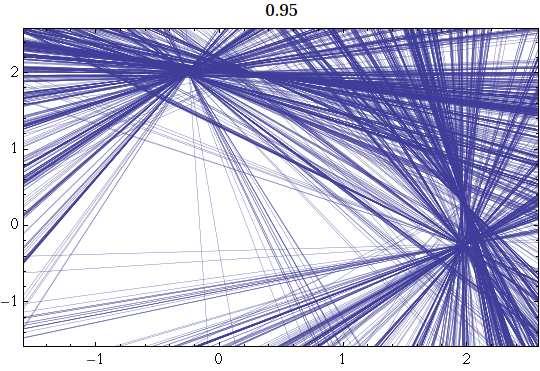
95 Figure 4.37: Left: line fields for b = 0.4; Right: b = 0.5 Figure 4.38: Left: line fields for b = 0.6; Right: b = 0.7 Figure 4.39: Left: line fields for b = 0.8; Right: b =