COMSOL Multiphysics Training. COMSOL Multiphysics

Transcription

1 COMSOL Multiphysics Training COMSOL Multiphysics

2

3

4 5. Products Chemical Field

5 CHEMICAL 1 - Chemical Reaction Engineering Chemical Reaction Engineering g Mass, Energy, and Momentum Transport

6 0D, very few unknowns. Fast (seconds). Idealized reacting systems. 3D Multiphysics. Detailed. Lots of unknowns. Heavy computations. Modeling Strategy Parameter estimation Space-independent Space-dependent Batch Reactor Semi-Batch Reactor CSTR Reactor Plug Flow Reactor Space-dependent 3D Porous Catalyst ci t c d dt i d uxci dx Dci uci Ri R i R i

7 Define Chemical Reaction Formulas in perfectly mixed environme nt (no change in space*) 2. The material balances for the species are automaticall y generated as you type in t he chemical equations 1. Just type in the chemical reaction form ulas 3. The kinetics are automatically formulat ed according to the law of mass action. If needed, you can replace the rat e law with your own expressions. Models for batch, semi-batch, continuous stirred tank reactors, and plug-flow reactors are predefin ed 4. Automatic units of rate consta nts, depending on kinetics expre ssions *The 1D plug flow reactor has no change in time Reaction Engineering Interface

8 with CAPE-OPEN(Thermodynaimcs) Run Simulation for the Perfectly Mixed System Parameter Estimation (with Optimization Module)

9 Transport Interfaces

10 Interactions Transport Phenomena Momentum Energy Mass Velocity(u) Pressure(p) rho mu Q Temperature(T) Cp rho k Convection Concentration(c) rho D R Convection CHEMKIN CAPE-OPEN Reaction Rate(R), Entalpy(H), Entropy(S), Heat Source(Q), Thermal Conductivity(k), Diffusion Coefficient(D), Density(rho), Heat Capacity(Cp), Viscosity(mu) Reaction Kinetics CHEMICAL 2 - Electrochemistry Electrochemistry Batteries & Fuel Cells Electrodeposition Corrosion osion

11 The Electrochemistry Interfaces Current Distribution Interfaces Generic Electrochemical Cell Modeling Nernst-Planck Equations Flat or porous electrodes Arbitrary number of reactions Electroanalysis Battery Interfaces (B&FC only) Corrosion Interfaces (Corrosion Module only) Electrodeposition Interfaces (Electrodeposition only) Electrochemical Reactions User-Defined Bulter-Volmer Linearized Bulter-Volmer Anodic Tafel equation Cathodic Tafel equation Concentration dependent kinetics Settings windows for electrode reactions for secondary current distribution

12 Electrodeposition & Corrosion Deformed Geometry With Moving Geometry Without Moving Geometry

13

14 Thermal Decomposition in a Parallel Plate Reactor Introductions outlet ROH R O OR Inlet Heated cylinder ROH Chemical Engineering Module Fully coupled momentum, energy and mass transport Strategies for Multiphysics modeling

15 Coupled Three phenomena Navier-Stokes Equations velocity Convection and Diffusion, Reaction Density,viscosity Thermal conductivity Heat capacity Reaction rate Temperature reaction rate =f(c) ( ) Convection and Conduction 1 One-way coupled The momentum transport is independent of the energy and mass transport The energy transport depends only on the momentum transport The mass transport depends on both the momentum transport and the energy transport The heat of reaction, Q, is neglected momentum Heat Mass

16 Momentum : Navier-stokes equations u u t 0 u T u u p F u Energy : Convection and Conduction C P T t kt Q C u T P T Mass : Convection and Diffusion c t i Dici Ri u ci R i E A exp RgT Ci c i 2 Fully Coupled The momentum transport depends on the energy transport The energy transport depends on both momentum and mass transport The mass transport depends on both the momentum transport and the energy transport momentum Heat Mass

17 Momentum : Navier-stokes equations u u t 0 u T u u p F u Energy : Convection and Conduction C P T t kt Q C u T P T Mass : Convection and Diffusion c t i Dici Ri u ci R i E A exp RgT Ci c i Model Navigator (Momentum / Heat / Mass Transport) / CAD (2D) omain / Boundary Settings (Momentum / Heat / Mass Transport) Mesh Solver Postprocessing

18 Coupled Three phenomena Navier-Stokes Equations velocity Convection and Diffusion, Reaction Density,viscosity Thermal conductivity Heat capacity Reaction rate Temperature reaction rate =f(c) ( ) Convection and Conduction Results - velocity < Constants > < T dependent >

19 Results - Temperature < Constants > < T dependent > Results - Concentration < Constants > < T dependent >

20 Thermal Decomposition Introduction In this tutorial, the heat and mass transport equations are coupled to laminar flow in order to model exothermic reactions in a parallel plate reactor. It exemplifies how you can use COMSOL Multiphysics to systematically set up and solve increasingly sophisticated models using predefined physics interfaces. Model Definition In this model you investigate the unimolecular decomposition of a chemical passing through a parallel plate reactor. A heat sensitive compound is present in a water solution. After entering the reactor, the liquid first experiences expansion due to a step in the bottom plate. Before exiting, the fluid also passes a heated cylinder. The full 3D representation of the reactor geometry is given in Figure 1. Top plate Outlet Inlet Heated cylinder Bottom plate Figure 1: 3D geometry of a parallel plate reactor. The reacting fluid is heated as it passes the cylinder. The short inlet section of the reactor is considerably wider than it is high. With such a geometry, it is reasonable to assume that the laminar flow develops a parabolic velocity profile between the top and bottom plate. At the same time, the velocity between the side walls is expected to be close to constant (Ref. 1). As a consequence, you can reduce the modeling domain to 2D without dramatically reducing the validity of the 1 THERMAL DECOMPOSITION

21 simulation (see Figure 2). Inlet Top plate Heating cylinder Outlet Bottom plate Figure 2: Neglecting edge effects, the modeling geometry can be reduced to 2D. CHEMISTRY A heat sensitive chemical (A) undergoes thermal decomposition into fragments (F) according to the following unimolecular reaction: A k F The reaction rate (SI unit: mol/(m 3 s)) is given by: rate = kc A where rate constant k (SI unit: s 1 ) is temperature dependent according to the Arrhenius equation: k = E Aexp R g T (1) In Equation 1, A is the frequency factor ( /s), E the activation energy ( J/mol), R g the gas constant (8.314 J/(mol K)), and T the temperature (SI unit: K). In addition, the decomposition reaction is exothermic, and the rate of energy expelled is given by: Q = rate H where H is the heat of reaction ( 100 kj/mol). The conversion of species A in the reactor is a function of the residence time; that is, it depends on the detailed fluid flow. Furthermore, the decomposition is influenced by the temperature distribution. A coupled system of transport equations thus describes the reactor. 2 THERMAL DECOMPOSITION

22 MOMENTUM TRANSPORT The Navier-Stokes equations, which govern momentum transport and are solved by default in the single-phase flow interfaces, give the compressible formulation of the continuity: ρ ( ρu) = 0 t (2) and the momentum equations: ρ u ρu u t = p μ( u + ( u) T 2 + ) --μ( u)i 3 + F (3) Here, μ denotes the dynamic viscosity (SI unit: Ns/m 2 ), u the velocity (SI unit: m/ s), ρ the density of the fluid (SI unit: kg/m 3 ), p the pressure (SI unit: Pa), and F a body force term (SI unit: N/m 3 ). This particular model contains the solution to a steady-state problem, so the first term in each of the equations above disappears. Equation 2 governs the flow of a Newtonian fluid in the laminar flow regime. The flow type in this specific model is determined in The Flow Regime. Apart from the domain equations you also need to select proper boundary conditions. At the inlet you specify a velocity vector normal to the boundary: u n = u 0 (4) At the outlet boundary you specify a pressure p = p 0. Finally, at the surfaces of the reactor plates and the heating cylinder you set the velocity to zero, that is, a no slip boundary condition: u = 0 (5) By selecting the Laminar Flow interface you can easily associate the momentum balance (Equation 2) and boundary conditions (Equation 4, Equation 5, and Equation 5) with your modeling geometry. ENERGY TRANSPORT The energy balance equation applied to the reactor domain considers heat transfer through convection and conduction: ( k T) + ρc p ( u )T = Q (6) 3 THERMAL DECOMPOSITION

23 In Equation 6, C p denotes the specific heat capacity (SI unit: J/(kg K)), k is the thermal conductivity (SI unit: W/(m K)), and Q is a sink or source term (SI unit: W/ m 3 ). At the inlet and at the surface of the heating cylinder you set a Temperature boundary condition: T = T 0 (7) T = T cyl (8) At the outlet you set an Outflow boundary condition. This prescribes that all energy passing through this boundary does so by means of convective transport. Equivalently, this means that the heat flux due to conduction across the boundary is zero: q cond n = k T n = 0 (9) so that the resulting equation for the total heat flux becomes: q n = ρc p T u n (10) This is a useful boundary condition, particularly in convection-dominated energy balances where the outlet temperature is unknown. Finally, assume that no energy is transported across the reactor plates, that is, apply a Thermal Insulation boundary condition: q n = 0 (11) Using the Heat Transfer in Fluids interface, you can associate the energy balance (Equation 6) and boundary conditions (Equation 7 to Equation 11) with the modeling geometry. MASS TRANSPORT The mass transfer in the reactor domain is given by the stationary convection and diffusion equation: ( D i c i ) + u c i = R i (12) where D i denotes its diffusion coefficient (SI unit: m 2 /s), and R i denotes the reaction term (SI unit: mol/(m 3 s)). Equation 12 assumes that the species i is diluted in a solvent. 4 THERMAL DECOMPOSITION

24 For the boundary conditions, specify the concentration of compound A at the inlet: c i = c i, 0 (13) At the outlet, specify that the mass flow through the boundary is dominated by convection. This assumes that any mass flux due to diffusion across this boundary is zero: n ( D i c i ) = 0 (14) and that: N i n = c i u n (15) Finally, at the surfaces of the reactor plates and the heating cylinder, assume that no mass is transported across the boundaries that is, an insulation boundary condition: N i n = 0 (16) By selecting the Transport in Diluted Species interface you can easily associate the mass balance (Equation 12) and boundary conditions (Equation 13 to Equation 16) with the modeling geometry. PREPARING FOR MODELING Before you can start modeling you need to gather the physical data that characterize your reacting flow. For instance, flow modeling requires you to supply the fluid density and viscosity. Mass transport requires knowledge of diffusivities and the reaction kinetics. Another part of the preparations involves selecting the appropriate physics interfaces and investigating the couplings between different transport equations. Transport Properties The term transport properties refers to the physical properties occurring in the transport equations (see the previous section). The momentum and heat transfer equations (Equation 2 and Equation 6) require fluid-specific transport properties: Viscosity (η) Density (ρ) Thermal conductivity (k) Heat capacity (C p ) 5 THERMAL DECOMPOSITION

25 The mass transport equation (Equation 12) requires the following species-specific property: Diffusivities (D i ) You need to supply appropriate values of the transport properties to the physics interfaces in order to ensure accurate simulation results. In the present example, water with the dissolved compound A enters the reactor at 300 K. Because water is the solvent, you can assume that its physical properties are representative for the entire fluid. The warmest part of the reactor is held at 325 K. Table 1 lists the transport properties of water as well as the diffusivity of A in water at 300 K and 325 K. TABLE 1: PHYSICAL PROPERTIES OF LIQUID WATER PROPERTY AT 300 K AT 325 K Density (kg/m 3 ) Viscosity (Ns/m 2 ) Thermal conductivity (W/(m K)) Heat capacity (J/(kg K)) Diffusivity (m 2 /s) When you build this model you make use of the built-in material databases of COMSOL Multiphysics, which automatically provides temperature-dependent properties. The Flow Regime The Reynolds number indicates whether a flow is in the laminar or turbulent regime: Re = ρud η As a rule of thumb, a Reynolds number between of 2000 and 2500 marks the transition from stable streamlines to stable turbulent flow. It is always good practice to evaluate the Reynolds number related to the specific flow conditions of the model, because its magnitude guides you to choose the appropriate flow model and corresponding physics interface. In the present example, you can evaluate the Reynolds number using values from Table 1 and setting the velocity to m/s and the characteristic length to m: Re = = 4 6 THERMAL DECOMPOSITION

26 Calculating the Reynolds number at 325 K produces a nearly identical result. The Reynolds numbers are well within the limits of the laminar flow regime. Dilute or Concentrated Mixtures When modeling mass transport, it is advisable to discriminate between dilute and concentrated mixtures. For dilute mixtures, Fick s Law is adequate to describe the diffusional transport. Furthermore, you can assume that the transport properties of the fluid are those of the solvent. For concentrated mixtures, on the other hand, other diffusion models, such as the Maxwell-Stefan model, may be required. The transport properties of the fluid then depend on the mixture composition. In COMSOL Multiphysics, the Transport of Diluted Species interface is appropriate for dilute mixtures, while the Transport of Concentrated Species interface is recommended for concentrated mixtures. As a rule of thumb, you can consider concentrations of up to 10 mol% of a solute in a solvent as a dilute mixture. In the example at hand, the compound A is dissolved in water at a concentration of 1000 mol/m 3. As the concentration of pure water is 55,500 mol/m 3, the molar fraction of A is approximately 2%. Because the mixture is dilute, it is appropriate to select the Transport of Diluted Species interface for mass transport and to select the transport properties of water as representative values for the mixture. Solving Coupled Models As noted previously, the chemistry occurring in the reactor depends both on the fluid flow and the temperature distribution in the reactor. More explicitly, the mass transport equation c i + ( D t i c i + c i u) = R i (17) depends on the velocity vector, u, which is solved for in the momentum transfer equation (Equation 3). Furthermore, the source term R i in Equation 17 is a function of the temperature, which in turn is the dependent variable of the energy transport equation ρc T p + ( k T ) + ρcp u T = Q t 7 THERMAL DECOMPOSITION

27 When attempting to solve a coupled system of equations such as the one illustrated above, it is often a good idea to analyze the couplings involved and then approach the solution in a stepwise fashion. In the current model, you first neglect the heat of reaction, Q. This leads to a loose two-way coupling between the transport equations: The momentum transport is weakly dependent on the energy and mass transport through the material properties. The energy transport depends only on the momentum transport. The mass transport depends on both the momentum transport and the energy transport. This structure suggests that it is possible to solve the problem sequentially in the following order: First solve the momentum transport and energy transport problem. Then add the mass transport and investigate the difference. The last step leads to a fully coupled problem: The momentum transport depends on the energy transport. The energy transport depends on both momentum and mass transport (added heat of reaction). The mass transport depends on both the momentum transport and the energy transport. In this case you must solve the equations describing all transport phenomena simultaneously. 8 THERMAL DECOMPOSITION

28 Results and Discussion Figure 3 shows the velocity field in the reactor domain along with arrows indicating the velocity magnitude. Figure 3: Velocity field (m/s) in the reactor. The cross-sectional area of the fluid increases at the step and decreases at the cylinder, leading to a corresponding local reduction and then increase in the fluid velocity. Recirculation zones appear after the step and the cylinder. 9 THERMAL DECOMPOSITION

29 The water solution enters the reactor at a temperature of 300 K and is heated as it passes the cylinder (325 K). Figure 4 shows the temperature distribution in the reactor domain at steady state. Figure 4: A water solution enters the reactor at 300 K and is heated by a cylinder kept at 325 K. 10 THERMAL DECOMPOSITION

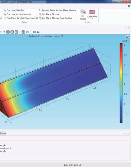
30 At the reactor inlet, the concentration of A is 1000 mol/m 3. Figure 5 shows the concentration of A as the compound undergoes decomposition. Figure 5: Concentration of the heat sensitive chemical (A) (mol/m 3 ) as function of position in the reactor. These plots make it possible to identify some general trends. It is clear that decomposition occurs mainly after the liquid has been heated by the cylinder. In the first half of the reactor, where the temperature is relatively low, decomposition is still fairly advanced near the wall and after the step. This is due to the longer residence times in these areas. In the second part of the reactor, where heating takes place, regions with relatively high concentrations of compound A are visible. This also makes physical sense because the water velocity is relatively high. The temperature distribution in the entire reactor is affected by the heat of reaction. As shown in Figure 6, the maximum fluid temperature now exceeds the temperature 11 THERMAL DECOMPOSITION

31 of the heating cylinder. Furthermore, the water temperature is higher than 300 K in the region between the inlet and the cylinder. Figure 6: Reactor temperature (K) when the heat of reaction is taken into account. 12 THERMAL DECOMPOSITION

32 Figure 7 plots the rate of reaction as a function of the position in the reactor. Clearly, significant reaction now occurs in the first part of the reactor, before the heating cylinder. Figure 7: Significant decomposition of compound A occurs in the first half of the reactor. Reference 1. H. Schlichting, Boundary Layer Theory, 4th ed., McGraw Hill, p. 168, Application Library path: Chemical_Reaction_Engineering_Module/ Reactors_with_Mass_and_Heat_Transfer/thermal_decomposition Modeling Instructions From the File menu, choose New. NEW 1 In the New window, click Model Wizard. 13 THERMAL DECOMPOSITION

33 MODEL WIZARD 1 In the Model Wizard window, click 2D. 2 In the Select physics tree, select Fluid Flow>Single-Phase Flow>Laminar Flow (spf). 3 Click Add. 4 Click Study. 5 In the Select study tree, select Preset Studies>Stationary. 6 Click Done. GLOBAL DEFINITIONS First define some parameters. Parameters 1 On the Home toolbar, click Parameters. 2 In the Settings window for Parameters, locate the Parameters section. 3 Click Load from File. 4 Browse to the application s Application Library folder and double-click the file thermal_decomposition_parameters.txt. GEOMETRY 1 Rectangle 1 (r1) 1 On the Geometry toolbar, click Primitives and choose Rectangle. 2 In the Settings window for Rectangle, locate the Size section. 3 In the Width text field, type W1. 4 In the Height text field, type H1. Rectangle 2 (r2) 1 On the Geometry toolbar, click Primitives and choose Rectangle. 2 In the Settings window for Rectangle, locate the Size section. 3 In the Width text field, type W2. 4 In the Height text field, type H2. Circle 1 (c1) 1 On the Geometry toolbar, click Primitives and choose Circle. 2 In the Settings window for Circle, locate the Size and Shape section. 3 In the Radius text field, type R1. 14 THERMAL DECOMPOSITION

34 4 Locate the Position section. In the x text field, type xpos. 5 In the y text field, type ypos. Difference 1 (dif1) 1 On the Geometry toolbar, click Booleans and Partitions and choose Difference. 2 Select the object r1 only to add it to the Objects to add list. 3 In the Settings window for Difference, locate the Difference section. 4 Find the Objects to subtract subsection. Select the Active toggle button. 5 Select the objects r2 and c1 only. 6 Right-click Component 1 (comp1)>geometry 1>Difference 1 (dif1) and choose Build Selected. ADD MATERIAL 1 On the Home toolbar, click Add Material to open the Add Material window. 2 Go to the Add Material window. 3 In the tree, select Liquids and Gases>Liquids>Water. 4 Click Add to Component in the window toolbar. 5 On the Home toolbar, click Add Material to close the Add Material window. MATERIALS Water (mat1) By default, the first material you add applies on all domains so you can keep the Geometric Scope settings. DEFINITIONS In preparation for defining boundary conditions, it is practical to define some named selections. Explicit 1 1 On the Definitions toolbar, click Explicit. 2 In the Model Builder window, under Component 1 (comp1)>definitions right-click Explicit 1 and choose Rename. 3 In the Rename Explicit dialog box, type Inlet in the New label text field. 4 Click OK. 5 In the Settings window for Explicit, locate the Input Entities section. 6 From the Geometric entity level list, choose Boundary. 15 THERMAL DECOMPOSITION

35 7 Select Boundary 1 only. Explicit 2 1 On the Definitions toolbar, click Explicit. 2 In the Model Builder window, under Component 1 (comp1)>definitions right-click Explicit 2 and choose Rename. 3 In the Rename Explicit dialog box, type Outlet in the New label text field. 4 Click OK. 5 In the Settings window for Explicit, locate the Input Entities section. 6 From the Geometric entity level list, choose Boundary. 7 Select Boundary 6 only. Explicit 3 1 On the Definitions toolbar, click Explicit. 2 In the Model Builder window, under Component 1 (comp1)>definitions right-click Explicit 3 and choose Rename. 3 In the Rename Explicit dialog box, type Heater in the New label text field. 4 Click OK. 5 In the Settings window for Explicit, locate the Input Entities section. 6 From the Geometric entity level list, choose Boundary. 7 Select Boundaries 7 10 only. Follow the instructions below to set up the Fluid Flow interface. The fluid properties are automatically taken from the material assigned to the reactor domain, so all you need to do is to define inlet and outlet boundary conditions. LAMINAR FLOW (SPF) Inlet 1 1 On the Physics toolbar, click Boundaries and choose Inlet. 2 In the Settings window for Inlet, locate the Boundary Selection section. 3 From the Selection list, choose Inlet. 4 Locate the Velocity section. In the U 0 text field, type 5e-4. Outlet 1 1 On the Physics toolbar, click Boundaries and choose Outlet. 2 In the Settings window for Outlet, locate the Boundary Selection section. 16 THERMAL DECOMPOSITION

36 3 From the Selection list, choose Outlet. 4 Locate the Pressure Conditions section. Select the Normal flow check box. This concludes the setup of the Laminar Flow interface. In the next step you will compute the solution. A mesh is created automatically. If you wish, you can inspect the mesh by clicking the Mesh node. STUDY 1 1 In the Model Builder window, right-click Study 1 and choose Rename. 2 In the Rename Study dialog box, type Isothermal Flow in the New label text field. 3 Click OK. 4 On the Home toolbar, click Compute. RESULTS Velocity (spf) 1 In the Model Builder window, under Results right-click Velocity (spf) and choose Arrow Surface. 2 On the Velocity (spf) toolbar, click Plot. 3 Click the Zoom Extents button on the Graphics toolbar. 4 In the Model Builder window, right-click Velocity (spf) and choose Rename. 5 In the Rename 2D Plot Group dialog box, type Flow Field in the New label text field. 6 Click OK. At this point, move on to include a Heat Transfer in Fluids interface and extend the model to account for a nonisothermal flow situation. ADD PHYSICS 1 On the Home toolbar, click Add Physics to open the Add Physics window. 2 Go to the Add Physics window. 3 In the Add physics tree, select Heat Transfer>Heat Transfer in Fluids (ht). 4 Find the Physics interfaces in study subsection. In the table, enter the following settings: Studies Isothermal Flow Solve 5 Click Add to Component in the window toolbar. 17 THERMAL DECOMPOSITION

37 6 On the Home toolbar, click Add Physics to close the Add Physics window. HEAT TRANSFER IN FLUIDS (HT) Temperature 1 1 On the Physics toolbar, click Boundaries and choose Temperature. 2 In the Settings window for Temperature, locate the Boundary Selection section. 3 From the Selection list, choose Inlet. 4 Locate the Temperature section. In the T 0 text field, type 300[K]. Temperature 2 1 On the Physics toolbar, click Boundaries and choose Temperature. 2 In the Settings window for Temperature, locate the Boundary Selection section. 3 From the Selection list, choose Heater. 4 Locate the Temperature section. In the T 0 text field, type 325[K]. Outflow 1 1 On the Physics toolbar, click Boundaries and choose Outflow. 2 In the Settings window for Outflow, locate the Boundary Selection section. 3 From the Selection list, choose Outlet. MULTIPHYSICS Couple the Laminar Flow interface to the Heat Transfer in Fluids interface, i.e., the pressure and velocity are inputs taken from the Laminar Flow interface 1 On the Physics toolbar, click Multiphysics and choose Global>Flow Coupling. Coupling the Heat Transfer in Fluids interface to the Laminar Flow interface, i.e., temperature is an input from the Heat Transfer in Fluids interface. 2 On the Physics toolbar, click Multiphysics and choose Global>Temperature Coupling. ADD STUDY 1 On the Home toolbar, click Add Study to open the Add Study window. 2 Go to the Add Study window. 3 Find the Studies subsection. In the Select study tree, select Preset Studies>Stationary. 4 Click Add Study in the window toolbar. 5 On the Home toolbar, click Add Study to close the Add Study window. 18 THERMAL DECOMPOSITION

38 STUDY 2 Step 1: Stationary 1 In the Settings window for Stationary, click to expand the Values of dependent variables section. 2 Locate the Values of Dependent Variables section. Select the Initial values of variables solved for check box. 3 From the Method list, choose Solution. 4 From the Study list, choose Isothermal Flow, Stationary. With this selection the solver will take the solution to the isothermal flow case as starting guess for the flow field and pressure variables. 5 In the Model Builder window, right-click Study 2 and choose Rename. 6 In the Rename Study dialog box, type Non-isothermal Flow in the New label text field. 7 Click OK. 8 In the Settings window for Study, locate the Study Settings section. 9 Clear the Generate default plots check box. 10 On the Home toolbar, click Compute. RESULTS 2D Plot Group 3 1 On the Home toolbar, click Add Plot Group and choose 2D Plot Group. 2 In the Settings window for 2D Plot Group, locate the Data section. 3 From the Data set list, choose Non-isothermal Flow/Solution 2. 4 Right-click Results>2D Plot Group 3 and choose Surface. 5 In the Settings window for Surface, click Replace Expression in the upper-right corner of the Expression section. From the menu, choose Component 1>Heat Transfer in Fluids>Temperature>T - Temperature. 6 On the 2D Plot Group 3 toolbar, click Plot. 7 In the Model Builder window, right-click 2D Plot Group 3 and choose Rename. 8 In the Rename 2D Plot Group dialog box, type Temperature in the New label text field. 9 Click OK. 19 THERMAL DECOMPOSITION

39 10 Click the Zoom Extents button on the Graphics toolbar. Now move on to extend the model to include mass transport and chemical reaction. ADD PHYSICS 1 On the Home toolbar, click Add Physics to open the Add Physics window. 2 Go to the Add Physics window. 3 In the Add physics tree, select Chemical Species Transport>Chemistry (chem). 4 Find the Physics interfaces in study subsection. In the table, enter the following settings: Studies Solve Isothermal Flow Non-isothermal Flow 5 Click Add to Component in the window toolbar. 6 In the Add physics tree, select Chemical Species Transport>Transport of Diluted Species (tds). 7 Click to expand the Dependent variables section. In the table, enter the following settings: Studies Solve Isothermal Flow Non-isothermal Flow 8 In the Concentrations table, enter the following settings: ca 9 Click Add to Component in the window toolbar. 10 On the Home toolbar, click Add Physics to close the Add Physics window. CHEMISTRY (CHEM) 1 In the Model Builder window, under Component 1 (comp1) click Chemistry (chem). 2 In the Settings window for Chemistry, locate the Model Inputs section. 3 From the T list, choose Temperature (ht). Reaction 1 1 On the Physics toolbar, click Domains and choose Reaction. 20 THERMAL DECOMPOSITION

40 2 In the Settings window for Reaction, locate the Reaction Formula section. 3 In the Formula text field, type A=>F. 4 Click Apply. 5 Locate the Rate Constants section. Select the Use Arrhenius expressions check box. 6 In the A f text field, type A. 7 In the E f text field, type E. 8 Locate the Reaction Thermodynamic Properties section. From the Enthalpy of reaction list, choose User defined. 9 In the H text field, type H. Species: F 1 In the Model Builder window, under Component 1 (comp1)>chemistry (chem) click Species: F. 2 In the Settings window for Species, click to expand the Species concentration/activity section. 3 Locate the Species Concentration/Activity section. Select the Locked concentration/ activity check box. TRANSPORT OF DILUTED SPECIES (TDS) On the Physics toolbar, click Chemistry (chem) and choose Transport of Diluted Species (tds). Transport Properties 1 1 In the Model Builder window, expand the Transport of Diluted Species (tds) node, then click Transport Properties 1. 2 In the Settings window for Transport Properties, locate the Diffusion section. 3 In the D ca text field, type 2e-9. Inflow 1 1 On the Physics toolbar, click Boundaries and choose Inflow. 2 In the Settings window for Inflow, locate the Boundary Selection section. 3 From the Selection list, choose Inlet. 4 Locate the Concentration section. In the c 0,cA text field, type Outflow 1 1 On the Physics toolbar, click Boundaries and choose Outflow. 2 In the Settings window for Outflow, locate the Boundary Selection section. 21 THERMAL DECOMPOSITION

41 3 From the Selection list, choose Outlet. Reactions 1 1 On the Physics toolbar, click Domains and choose Reactions. 2 Select Domain 1 only. 3 In the Settings window for Reactions, locate the Reaction Rates section. 4 From the R ca list, choose Rate expression for species A (chem). The chemical reaction generates heat. Take this into account by adding a Heat Source node to the Heat Transfer in Fluids interface. HEAT TRANSFER IN FLUIDS (HT) Heat Source 1 1 On the Physics toolbar, click Domains and choose Heat Source. 2 Select Domain 1 only. 3 In the Settings window for Heat Source, locate the Heat Source section. 4 From the Q 0 list, choose Heat source of reactions (chem). MULTIPHYSICS Couple the Laminar Flow interface to the Transport of Diluted Species interface, i.e., the velocity is an input from the Laminar Flow interface. 1 On the Physics toolbar, click Multiphysics and choose Global>Flow Coupling. 2 In the Settings window for Flow Coupling, locate the Flow Coupling section. 3 From the Destination list, choose Transport of Diluted Species (tds). Couple the Heat Transfer in Fluids interface to the Transport of Diluted Species interface, i.e., temperature is an input from the Heat Transfer in Fluids interface. 4 On the Physics toolbar, click Multiphysics and choose Global>Temperature Coupling. 5 In the Settings window for Temperature Coupling, locate the Temperature Coupling section. 6 From the Destination list, choose Transport of Diluted Species (tds). ADD STUDY 1 On the Home toolbar, click Add Study to open the Add Study window. 2 Go to the Add Study window. 3 Find the Studies subsection. In the Select study tree, select Preset Studies>Stationary. 22 THERMAL DECOMPOSITION

42 4 Click Add Study in the window toolbar. 5 On the Home toolbar, click Add Study to close the Add Study window. STUDY 3 Step 1: Stationary 1 In the Model Builder window, under Study 3 click Step 1: Stationary. 2 In the Settings window for Stationary, click to expand the Values of dependent variables section. 3 Locate the Values of Dependent Variables section. Select the Initial values of variables solved for check box. 4 From the Method list, choose Solution. 5 From the Study list, choose Non-isothermal Flow, Stationary. 6 In the Model Builder window, right-click Study 3 and choose Rename. 7 In the Rename Study dialog box, type Fully Coupled in the New label text field. 8 Click OK. 9 In the Settings window for Study, locate the Study Settings section. 10 Clear the Generate default plots check box. 11 On the Home toolbar, click Compute. RESULTS Temperature 1 In the Settings window for 2D Plot Group, locate the Data section. 2 From the Data set list, choose Fully Coupled/Solution 3. 3 Click the Zoom Extents button on the Graphics toolbar. 4 On the Temperature toolbar, click Plot. Create new plot groups and generate surface plots for the concentration and the reaction rate. 2D Plot Group 4 1 On the Home toolbar, click Add Plot Group and choose 2D Plot Group. 2 In the Settings window for 2D Plot Group, locate the Data section. 3 From the Data set list, choose Fully Coupled/Solution 3. 4 Right-click Results>2D Plot Group 4 and choose Surface. 23 THERMAL DECOMPOSITION

43 5 In the Settings window for Surface, click Replace Expression in the upper-right corner of the Expression section. From the menu, choose Component 1>Transport of Diluted Species>cA - Concentration. 6 On the 2D Plot Group 4 toolbar, click Plot. 7 Click the Zoom Extents button on the Graphics toolbar. 8 In the Model Builder window, right-click 2D Plot Group 4 and choose Rename. 9 In the Rename 2D Plot Group dialog box, type Concentration in the New label text field. 10 Click OK. 2D Plot Group 5 1 On the Home toolbar, click Add Plot Group and choose 2D Plot Group. 2 In the Settings window for 2D Plot Group, locate the Data section. 3 From the Data set list, choose Fully Coupled/Solution 3. 4 Right-click Results>2D Plot Group 5 and choose Surface. 5 In the Settings window for Surface, click Replace Expression in the upper-right corner of the Expression section. From the menu, choose Component 1>Transport of Diluted Species>tds.R_cA - Total rate expression. 6 On the 2D Plot Group 5 toolbar, click Plot. 7 Click the Zoom Extents button on the Graphics toolbar. 8 In the Model Builder window, right-click 2D Plot Group 5 and choose Rename. 9 In the Rename 2D Plot Group dialog box, type Reaction Rate in the New label text field. 10 Click OK. 24 THERMAL DECOMPOSITION

44

45 Optimization of a Catalytic Microreactor

46

47 Optimization of a Catalytic Microreactor Introduction In this example model, a solution is pumped through a catalytic bed, where a reactant undergoes chemical reaction as it gets in contact with the catalyst. The purpose of the model is to maximize the total reaction rate for a given total pressure difference across the bed by finding an optimal catalyst distribution. The distribution of the porous catalyst determines the total reaction rate in the bed. A large amount of catalyst results in a low flow rate through the bed while less catalyst gives a high flow rate but low conversion of the reactant. This modeling example is based on Ref. 1. Note: This application requires the Optimization Module. Model Definition The model geometry is shown in Figure 1. The reactor consists of an inlet channel, a fixed catalytic bed, and an outlet channel. 1 OPTIMIZATION OF A CATALYTIC MICROREACTOR

48 Reacting domain Inlet Outlet Symmetry boundary Figure 1: Model geometry. The optimal catalyst distribution should maximize the average reaction rate, which is expressed as the integral of the local reaction rate, r (SI unit: mol/(m 3 s)), over the domain, Ω. This is equivalent to minimizing the negative of this average reaction rate: 1 min r dω vol(ω) Assuming a first-order catalytic reaction with respect to the reactant species, the local reaction rate is determined by Ω r = k a ( 1 ε)c (1) where ε denotes the volume fraction of solid catalyst, c refers to the concentration (SI unit: mol/m 3 ), and k a is the rate constant (SI unit: 1/s). The mass transport is described by the convection and diffusion equation ( D c) = r u c where u denotes the velocity vector (SI unit: m/s) and D is the diffusion coefficient (SI unit: m 2 /s). The Navier-Stokes equations describe the fluid flow: ρ( u )u = p + μ u ( + ( u) T ) α( ε)u u = 0 (2) 2 OPTIMIZATION OF A CATALYTIC MICROREACTOR

49 The coefficient α(ε) depends on the distribution of the porous catalyst as αε ( ) = μ q( 1 ε) Da L q + ε (3) where Da is the Darcy number; L is the length scale (SI unit: m); and q is a dimensionless parameter, the interpretation of which is discussed in the next section. From Equation 3, the direct conclusion is that when ε equals 1, α equals zero and Equation 2 reduces to the ordinary Navier-Stokes equations. In this case the reaction rate is zero; see Equation 1. To summarize, the optimization problem is 1 min k vol(ω) ( a ( 1 ε)c) dω ε Ω (4) where ρ( u )u = p + μ u ( + ( u) T ) α( ε)u u = 0 and physical boundary conditions apply. ( D c) = r u c 0 ε 1 CONVEX OPTIMIZATION PROBLEMS One of the most important characteristics of an optimization problem is whether or not the problem is convex. This section therefore briefly describes this property. For a more general discussion of the subject, see for example Ref. 2. A set C is said to be convex if for any two members x, y of C, the following relation holds: tx + ( 1 t)y C for every t [ 01, ] that is, the straight line between x and y is fully contained in C. A convex function is a mapping f from a convex set C such that for every two members x, y of C ftx ( + ( 1 t)y) tf( x) + ( 1 t)fy ( ) for every t [ 0, 1] (5) 3 OPTIMIZATION OF A CATALYTIC MICROREACTOR

50 An optimization problem is said to be convex if the following conditions are met: the design domain is convex the objective and constraints are convex functions The importance of convexity follows simply from the result that if x* is a local minimum to a convex optimization problem, then x* is also a global minimum. This is easily proven by simply assuming that there is a y such that f(y) < f(x*), and then using Equation 5. This particular optimization problem is nonlinear, because a change in ε implies a change in the concentration, c. Because of this implicit dependence, it is very difficult to determine whether or not the objective is convex. There is therefore no guarantee that the optimal solution you obtain is globally optimal or unique. In the best of cases, running the optimization gives a good local optimum. The parameter q can be used to smoothen the interfaces between the catalyst and the open channel. To see the effect of this parameter, rewrite Equation 3 as αε ( ) = μ 1 ε Da L ε q 4 OPTIMIZATION OF A CATALYTIC MICROREACTOR

51 It follows that when q approaches infinity, α is the (inverse) porosity. On the other hand, lowering the value of q decreases the magnitude of α. Figure 2: q(1 ε)/(q ε) plotted as a function of ε for different values of q. Figure 2 shows q(1 ε)/(q ε) plotted as a function of ε for different values of q. This plot shows that lowering the value of q, increases the convexity of the force coefficient. For a low q value, an increase in ε around 0.5, imposes a small increase of the force coefficient, while for a higher value of q, a change in ε imposes an almost equal change for the whole range. Therefore, for a lower q value, the solution is not sharp at the interfaces. On the other hand, for small values of ε, the force term decreases rapidly when q is small, and thus affects the flow field to a much wider extent. In the limit when q approaches infinity, α as a function of ε is a straight line. Results and Discussion Figure 3 shows the velocity field in the empty channel, this is the starting point for the optimization. 5 OPTIMIZATION OF A CATALYTIC MICROREACTOR

52 Figure 3: Velocity field in the open channel. Figure 4: Distribution of the porous catalyst seen in black and open channel in white. 6 OPTIMIZATION OF A CATALYTIC MICROREACTOR

53 Figure 4 shows the distribution of the porous catalyst in black and the open channels in white. This result shows that, optimally, the supply of the reactant should be distributed over a large area of the reactor. Note also that the amount of open channel volume is significant. Figure 5 shows the concentration distribution in the reactor. This plot shows how the porous catalyst is fed with the reactant through the open channels. The plot naturally resembles that of Figure 4. Figure 5: Concentration distribution in the reactor after optimization. Let F i = n flow ( D c + cu) ds Ω i where n flow refers to the normal to the boundary Ω i in the flow direction (that is, pointing in to the domain at the inlet and out from the domain at the outlet). Then F i is a measurement of the flow of the species with concentration c through the boundary Ω i per unit length in the transverse dimension. The conversion, X, of the reactant is defined as 7 OPTIMIZATION OF A CATALYTIC MICROREACTOR

54 X = F in F out F in In this case, the conversion of the reactant is around 50%. Figure 6 shows the velocity field in the reactor. The porous catalyst slows down the flow significantly compared to Figure 3. Figure 6: Velocity field in the reactor after optimization. References 1. F. Okkels and H. Bruus, Scaling Behavior of Optimally Structured Catalytic Microfluidic Reactors, Phys. Rev. E, vol. 75, pp , S.G. Nash and A. Sofer, Linear and Nonlinear Programming, McGraw-Hill, Application Library path: Chemical_Reaction_Engineering_Module/ Reactors_with_Mass_Transfer/microreactor_optimization 8 OPTIMIZATION OF A CATALYTIC MICROREACTOR

55 Modeling Instructions From the File menu, choose New. NEW 1 In the New window, click Model Wizard. MODEL WIZARD 1 In the Model Wizard window, click 2D. 2 In the Select physics tree, select Fluid Flow>Single-Phase Flow>Laminar Flow (spf). 3 Click Add. 4 In the Select physics tree, select Chemical Species Transport>Transport of Diluted Species (tds). 5 Click Add. 6 In the Select physics tree, select Mathematics>Optimization and Sensitivity>Optimization (opt). 7 Click Add. 8 Click Study. 9 In the Select study tree, select Preset Studies for Selected Physics Interfaces>Stationary. 10 Click Done. GLOBAL DEFINITIONS Parameters 1 On the Home toolbar, click Parameters. 2 In the Settings window for Parameters, locate the Parameters section. 3 In the table, enter the following settings: Name Expression Value Description q Optimization parameter Da 1e-4 1E-4 Darcy number L 1[mm] m Length scale rho 1000[kg/m^3] 1000 kg/m³ Density of water eta 1e-3[Pa*s] Pa s Viscosity of water c_in 1[mol/m^3] 1 mol/m³ Concentration at inlet 9 OPTIMIZATION OF A CATALYTIC MICROREACTOR

56 Name Expression Value Description k_a 0.25[mol/ (m^3*s)] 0.25 mol/(m³ s) Reaction rate coefficient delta_p 0.25[Pa] 0.25 Pa Pressure drop vol 3*L*6*L 1.8E-5 m² Volume of the reacting domain D 3e-8[m^2/s] 3E-8 m²/s Diffusion coefficient GEOMETRY 1 Next, create the geometry. The reactor consists of three domains: the inlet channel, the reacting domain, and the outlet channel (see Figure 1). 1 In the Model Builder window, under Component 1 (comp1) click Geometry 1. 2 In the Settings window for Geometry, locate the Units section. 3 From the Length unit list, choose mm. Rectangle 1 (r1) 1 On the Geometry toolbar, click Primitives and choose Rectangle. 2 In the Settings window for Rectangle, locate the Size section. 3 In the Width text field, type 2*L. 4 In the Height text field, type L. Rectangle 2 (r2) 1 On the Geometry toolbar, click Primitives and choose Rectangle. 2 In the Settings window for Rectangle, locate the Size section. 3 In the Width text field, type 6*L. 4 In the Height text field, type 3*L. 5 Locate the Position section. In the x text field, type 2*L. Rectangle 3 (r3) 1 On the Geometry toolbar, click Primitives and choose Rectangle. 2 In the Settings window for Rectangle, locate the Size section. 3 In the Width text field, type 2*L. 4 In the Height text field, type L. 5 Locate the Position section. In the x text field, type 8*L. 6 Right-click Component 1 (comp1)>geometry 1>Rectangle 3 (r3) and choose Build Selected. 10 OPTIMIZATION OF A CATALYTIC MICROREACTOR

57 7 Click the Zoom Extents button on the Graphics toolbar. The geometry should now look like that in Figure 1. DEFINITIONS Define integration couplings to use for calculating the conversion of the reactant. Integration 1 (intop1) 1 On the Definitions toolbar, click Component Couplings and choose Integration. 2 In the Settings window for Integration, locate the Source Selection section. 3 From the Geometric entity level list, choose Boundary. 4 Select Boundary 1 only. Integration 2 (intop2) 1 On the Definitions toolbar, click Component Couplings and choose Integration. 2 In the Settings window for Integration, locate the Source Selection section. 3 From the Geometric entity level list, choose Boundary. 4 Select Boundary 12 only. Variables 1 1 On the Definitions toolbar, click Local Variables. 2 In the Settings window for Variables, locate the Variables section. 3 In the table, enter the following settings: Name Expression Unit Description F_in intop1(tds.tflux_cx mol/(m s) Influx ) F_out intop2(tds.tflux_cx ) mol/(m s) Outflux X (F_in-F_out)/F_in Conversion of reactant Here, tds.tfluxx_c is the COMSOL Multiphysics variable for the x-component of the total flux. Variables 2 1 On the Definitions toolbar, click Local Variables. 2 In the Settings window for Variables, locate the Geometric Entity Selection section. 3 From the Geometric entity level list, choose Domain. 4 Select Domain 2 only. 11 OPTIMIZATION OF A CATALYTIC MICROREACTOR

58 5 Locate the Variables section. In the table, enter the following settings: Name Expression Unit Description phi k_a*(1-epsilon)*c Local reaction rate alpha (eta/ (Da*L^2))*q*(1-epsi lon)/(q+epsilon) Drag-force coefficient ADD MATERIAL 1 On the Home toolbar, click Add Material to open the Add Material window. 2 Go to the Add Material window. 3 In the tree, select Built-In>Water, liquid. 4 Click Add to Component in the window toolbar. 5 On the Home toolbar, click Add Material to close the Add Material window. LAMINAR FLOW (SPF) Volume Force 1 1 On the Physics toolbar, click Domains and choose Volume Force. 2 Select Domain 2 only. 3 In the Settings window for Volume Force, locate the Volume Force section. 4 Specify the F vector as -alpha*u -alpha*v x y Inlet 1 1 On the Physics toolbar, click Boundaries and choose Inlet. 2 Select Boundary 1 only. 3 In the Settings window for Inlet, locate the Boundary Condition section. 4 From the list, choose Pressure. 5 Locate the Pressure Conditions section. In the p 0 text field, type delta_p. Symmetry 1 1 On the Physics toolbar, click Boundaries and choose Symmetry. 2 Select Boundaries 2, 5, and 9 only. 12 OPTIMIZATION OF A CATALYTIC MICROREACTOR

59 Outlet 1 1 On the Physics toolbar, click Boundaries and choose Outlet. 2 Select Boundary 12 only. TRANSPORT OF DILUTED SPECIES (TDS) Transport Properties 1 1 In the Model Builder window, expand the Component 1 (comp1)>transport of Diluted Species (tds) node, then click Transport Properties 1. 2 In the Settings window for Transport Properties, locate the Model Inputs section. 3 From the u list, choose Velocity field (spf). 4 Locate the Diffusion section. In the D c text field, type D. Reactions 1 1 On the Physics toolbar, click Domains and choose Reactions. 2 Select Domain 2 only. 3 In the Settings window for Reactions, locate the Reaction Rates section. 4 In the R c text field, type -phi. Concentration 1 1 On the Physics toolbar, click Boundaries and choose Concentration. 2 In the Settings window for Concentration, locate the Concentration section. 3 Select the Species c check box. 4 In the c 0,c text field, type c_in. 5 Select Boundary 1 only. Outflow 1 1 On the Physics toolbar, click Boundaries and choose Outflow. 2 Select Boundary 12 only. This completes the setup of the physics. Now set up the optimization problem. OPTIMIZATION (OPT) Define the control variable epsilon, select its shape, and constrain its values to the interval [0, 1]. Control Variable Field 1 1 On the Physics toolbar, click Domains and choose Control Variable Field. 13 OPTIMIZATION OF A CATALYTIC MICROREACTOR

60 2 Select Domain 2 only. Because the porous catalyst is only used in the reacting domain you can deactivate the inlet and outlet channels. 3 In the Settings window for Control Variable Field, locate the Control Variable section. 4 In the Control variable name text field, type epsilon. 5 In the Initial value text field, type 1. 6 Locate the Discretization section. From the Element order list, choose Linear. Control Variable Bounds 1 1 In the Model Builder window, right-click Control Variable Field 1 and choose Control Variable Bounds. 2 In the Settings window for Control Variable Bounds, locate the Bounds section. 3 In the Upper bound text field, type 1. Next, define the objective function. Integral Objective 1 1 On the Physics toolbar, click Domains and choose Integral Objective. 2 Select Domain 2 only. 3 In the Settings window for Integral Objective, locate the Objective section. 4 In the Objective expression text field, type -phi/vol. This example requires a fine mesh, both to solve the physics problem and to resolve the topology optimization problem. MESH 1 1 In the Model Builder window, under Component 1 (comp1) click Mesh 1. 2 In the Settings window for Mesh, locate the Mesh Settings section. 3 From the Element size list, choose Finer. 4 Click the Build All button. STUDY 1 Although you can choose to solve the optimization problem directly, it can be useful to check that the solution for the PDE problem looks sound before starting the optimization. 1 On the Home toolbar, click Compute. 14 OPTIMIZATION OF A CATALYTIC MICROREACTOR

61 RESULTS Velocity (spf) The first default plot (see Figure 3) shows the velocity field in the reactor. Now solve the optimization problem. STUDY 1 Step 1: Stationary 1 In the Model Builder window, expand the Study 1 node, then click Step 1: Stationary. 2 In the Settings window for Stationary, click to expand the Results while solving section. 3 Locate the Results While Solving section. Select the Plot check box. This setting gives a plot of the evolving velocity distribution in the Graphics window. Optimization 1 On the Study toolbar, click Optimization. Choose the SNOPT solver rather than MMA since the objective function contains an implicit trade-off between a high flow rate and a high active catalyst area. This makes the objective severely nonlinear. 2 In the Settings window for Optimization, locate the Optimization Solver section. 3 From the Method list, choose SNOPT. Solution 1 1 On the Study toolbar, click Show Default Solver. 2 In the Model Builder window, expand the Solution 1 node. 3 In the Model Builder window, expand the Study 1>Solver Configurations>Solution 1>Optimization Solver 1 node, then click Stationary 1. 4 In the Settings window for Stationary, locate the General section. 5 In the Relative tolerance text field, type 1e-6. 6 On the Study toolbar, click Compute. RESULTS Velocity (spf) The velocity field in the reactor after optimization should resemble that in Figure OPTIMIZATION OF A CATALYTIC MICROREACTOR

62 Concentration (tds) The third default plot shows the concentration distribution in the reactor after optimization (Figure 5). To reproduce the plot in Figure 4, modify the default plot with the following steps. 2D Plot Group 4 1 In the Model Builder window, under Results click 2D Plot Group 4. 2 In the Settings window for 2D Plot Group, click to expand the Title section. 3 From the Title type list, choose Manual. 4 In the Title text area, type Distribution of porous catalyst. 5 In the Model Builder window, expand the 2D Plot Group 4 node, then click Surface 1. 6 In the Settings window for Surface, click Replace Expression in the upper-right corner of the Expression section. From the menu, choose Component 1>Optimization>epsilon - Control variable epsilon. 7 Locate the Coloring and Style section. From the Color table list, choose GrayScale. 8 Clear the Color legend check box. 9 On the 2D Plot Group 4 toolbar, click Plot. 10 Click the Zoom Extents button on the Graphics toolbar. 11 Right-click Results>2D Plot Group 4>Surface 1 and choose Rename. 12 In the Rename Surface dialog box, type Porous Catalyst in the New label text field. 13 Click OK. 14 Click the Zoom Extents button on the Graphics toolbar. Derived Values To display the result for the conversion rate, continue as follows: 1 On the Results toolbar, click Global Evaluation. 2 In the Settings window for Global Evaluation, click Replace Expression in the upper-right corner of the Expression section. From the menu, choose Component 1>Definitions>Variables>X - Conversion of reactant. 3 Click the Evaluate button. TABLE 1 Go to the Table window. The value appears in the Table window below the Graphics window. 16 OPTIMIZATION OF A CATALYTIC MICROREACTOR

63

64 Wire Electrode Modeling of Electrochemical Cells Primary current distribution Accounts only for Ohmic effects in the simulation of current density distribution and performance of the cell: Neglects the influence of concentration variations in the electrolyte Neglects the influence of electrode kinetics on the performance of the cell, i.e. activation o verpotential is neglected (losses due to activation energy) Secondary current distribution Accounts only for Ohmic effects and the effect of electrode kinetics in the simul ation of current density distribution and performance of the cell: Neglects the influence of concentration variations in the electrolyte Tertiary current distribution Accounts for Ohmic effects, effects of electrode kinetics, and the effects of conc entration variations on the performance of a cell

65 Modeling of Electrochemical Cells Non-porous electrodes Heterogeneous reactions Typically used for electrolysis, metal winning, and electrodeposition Porous electrodes Reactions treated as homogeneous reaction in models although they are heterogeneous in reality Typically used for batteries, fuel cells, and in some cases also for electrolysis Electrolytes Diluted and supporting electrolytes Concentrated electrolytes Free electrolytes with forced and free convection Immobilized electrolytes through the use of porous matrixes, negligible free convection, rarely force d convection Solid electrolytes, no convection Primary Current Distribution Assumptions: Perfectly mixed electrolyte Negligible activation overpotential Negligible ohmic losses in the anode structure Anode: Wire electrode Cathodes: Flat-plate electrodes Cathodes: Flat-plate electrodes Electrolyte

66 Domain and Boundary Settings Domain: Charge continuity Boundary Electrode potentials at electrode surfaces Insulation elsewhere Cathodes: Electrode potential = 0 V E 0 = 0 V (negligible overpotential) Anode: Cell voltage = 1.3 V E 0 = 1.2 V Total cell (in this case ohmic) polarization = 100 mv Cathodes: 0 V Electrolyte: 0 l Ionic potential l Some Definitions Activation and concentration over potential = 0 0 s l E 0 l s E 0 Select the cathode as reference p oint sc, 0 E cell s, a s, c 0 E lc, 0, c E E l, a cell 0, a Ionic potential l Electronic potential s Ecell a c Cell voltage At anode, index At cathode, index

67 Results Current density distribution at tha anode surface Potential distribution in the electrolyte Highly active catalyst Inactive catalyst Secondary Current Distribution Activation overpotential taken int oaccount s l E 0 Charge transfer current at the elec trode surfaces New boundary conditions l n ict 1 F F ict i 0 exp exp RT g RT g Exchange current density Faraday s constant Gas constant Charge transfer coefficient

68 Comparison: Primary and Secondary C urrent Distributions Current density distribution at the anode surface Polarization curves Solid line = Primary Dashed line = Secondary Effect of Activation overpotential Lower current density with equal cell voltage (1.3V) compared to primary case Comparison: Primary and Secondary Current Density Dis tribution, 0.1 A Total Current Dimensionless current density disr ibution, primary case Dimensionless current density disr ibution, secondary case Independent of total current Dependent of total current cdd i i ct ct, average

69 Tertiary Current Density Distribution Use the secondary current distribution case as starting point Add the flow equations, in this case from single phase laminar flow Navier-Stokes Solve only for the flow Add equations for mass transport, in this chase the Nernst-Planck equations Introduce the concentration dependence on the reaction kinetics Solve the fully coupled material and charge balances using the already solved flow fi eld Results: Concentration and Current De nsity Distribution Main direction of the flow Stagnation in the flow results in lower concentration

70 Comparison: Primary, Secondary, Tertiary Current Distributions

71 Wire Electrode Solved with COMSOL Multiphysics 5.1 One of the most important aspects in the design of electrochemical cells is the current density distributions in the electrolyte and electrodes. Non-uniform current density distributions can be detrimental for the operation of electrochemical processes. In many cases the parts of an electrode that are subjected to high current density degrade at a faster rate. Knowledge of the current density distribution is also desired to optimize the utilization of the electrocatalysts, because these are often made of expensive noble metals. Non-uniform deposition and consumption, as well as unnecessarily high overvoltages, with resulting energy losses and possibly unwanted side-reactions, may be other effects that one would like to minimize. This example models the primary, secondary, and tertiary current density distributions (Ref. 1) of an arbitrary electrochemical cell. It successively goes through the different classes of current density distributions so as to also show how complexity should be gradually introduced when modeling electrochemical cells. Introduction The same geometry is considered in all three cases: a wire electrode structure is placed between two flat electrode surfaces, and in the open volume between the wire and the flat surfaces electrolyte is allowed to flow; see Figure 1. The electrochemical cell can be seen as a unit cell of a larger wire-mesh electrode an electrochemical cell setup common for many large-scale industrial processes. 1 WIRE ELECTRODE

72 . Flat electrode (cathode) Wire electrode (anode) Outlet Flat electrode (cathode) Inlet Figure 1: Modeled electrochemical cell. Wire electrode (anode) between two flat electrodes (cathodes). Flow inlet to the left, outlet to the right. The top and bottom flat surfaces are inert. Model Definition PRIMARY CURRENT DISTRIBUTION Figure 1 shows the investigated geometry. Firstly, this example considers primary current density distribution. This is the situation where the mixing of electrolyte is vigorous or where concentration gradients are small, so that ionic migration is the dominating transport mechanism. The general mass balance in the electrolyte, assuming steady-state conditions and that no homogeneous reactions occur, can be given by N i = 0 where N i is the flux of species i (SI unit: mol m 2 /s), which in turn is governed by: D i c i z i m i Fc i φ l + c i u = N i (1) where c i represents the concentration of the ion i (SI unit: mol/m 3 ), z i its valence, D i its diffusivity (SI unit: m 2 /s), m i its mobility (SI unit: mol m 2 (s V A)), F denotes the 2 WIRE ELECTRODE

73 Faraday constant (SI unit: As/mol), φ i the ionic potential, and u the velocity vector (SI unit: m/s). The components operated upon by the above transport equation are often described as the diffusion, migration, and convection transport mechanisms. The net current density can be described through: where i is the current density vector (SI unit: A/m 2 ). Combining the three above equations, while assuming electroneutrality (which removes the convection term) and negligible concentration gradients (which removes diffusion) leaves: Current density is conserved throughout: i = F z i N i 2 i = F z m i i Fc i φ l i = 0 (2) so that by combining the valence, ionic mobility, constant concentration and the Faraday constant to a representative conductivity, κ (SI unit: 1/(W m 2 )), Equation 2 becomes: ( κ φ l ) = 0 (3) This final equation is basically Ohm s Law. The boundary conditions for the case of primary current density distribution assume that the kinetics on the electrode surfaces are fast, which allow the assumption of constant potential on these surfaces (all other boundaries are insulated). The solid phase (electronic conductor) potential on the cathode, convenient choice of reference potential in the system: φ s, c = 0 (SI unit: V), is a The electrode potential equals the difference between the potential of solid phase in the electrode,, and the potential in the adjacent electrolyte, : φ e E electrode = φ s φ l In the absence of kinetic losses, the cathode potential, E c, equals the equilibrium potential, E eq,c : E eq, c φ s, c φ l, c φ s, c = = φ l, c φ i 3 WIRE ELECTRODE

74 which sets the boundary condition for the cathode. The potential difference over the whole cell, E cell, is defined as the potential difference between the solid phases of the two electrodes E cell = φ s, a φ s, c = φ s, a In this way the boundary condition for the ionic potential at the anode can be set via: E eq, a φ s, a φ l, a = = E cell φ l, a SECONDARY CURRENT DISTRIBUTION Secondary current distribution takes into account the kinetics at the electrodes. Mixing is supposed to be good and the electroneutrality condition still relevant so that Ohm s Law remains a good description for the equations in the domain. Yet the electrochemical reactions are no longer fast enough that a constant potential can be applied at the electrodes. The properties of the chemical species and their ability to react at the surface, that is, the reaction driving forces (overvoltages), need to be considered. In this model, the expressions for the local current density, i (SI unit: A/m 2 ), is based on the Butler-Volmer equation (Ref. 2) for a single electron reaction. For the secondary current distribution case (that is, without concentration dependence) it reads: i loc = i 0 ( exp( η( 1 β)f ( RT) ) exp( ηβf ( RT) )) here T is the temperature and R is the gas constant (SI unit: J/(K mol). i 0, the exchange current density, (SI unit: A/m 2 ), and β, the symmetry factor, are reaction and electrode dependent and are therefore different for each electrode. The overpotential, η, is the difference between the electrode potential and the equilibrium potential for the electrode reaction, defined in the following way: η = E electrode E eq This results in the following expressions for the overpotentials for the cathode and anode, respectively: η c = φ l, c E eq, c η a = E cell φ l, a E eq, a 4 WIRE ELECTRODE

75 TERTIARY CURRENT DISTRIBUTION In tertiary current density distribution, mass transport through diffusion, convection, and migration has to be considered (that is, all components of Equation 1). For the net ionic charge transport the assumption for this model still is electroneutrality and a supporting electrolyte with negligible concentration gradients, which means that the potential distribution in the electrolyte can be described through Ohm s Law (Equation 3) To introduce a mass transport dependence in this model the species being oxidized at the anode now has mass transport limitations and its localized concentration, c (SI unit: mol/m 3 ), affects the electrode kinetics. The anodic branch of the Butler-Volmer expression at the anode therefore gets a concentration dependence, and the expression now reads: c i a = i exp( η( 1 β)f ( RT) ) exp( ηβf ( RT) ) c 0 (4) Here c 0 (SI unit: mol/m 3 ) denotes a reference concentration (equal to the inlet concentration). Equation 4 is applied to the wire (anode) electrode, while the cathodes keep the expression for the local current density from the secondary current distribution model. Also a momentum balance is introduced to describe the convection. In this case, the assumption is a stationary laminar incompressible flow, using the Navier-Stokes equation: μ( u + ( u) T ) + ρ( u )u + p = 0 u = 0 (5) where μ is the dynamic viscosity (SI unit: Ns/m 2 ), ρ density (SI unit: kg/m 3 ) and p pressure (SI unit: Pa). No Slip boundary conditions are applied to the electrode surfaces, and slip boundary conditions to the top and bottom to account for the periodically repeating unit cell in this spatial direction. At the inlet, a laminar inflow with a fixed mean velocity is specified, whereas a pressure condition specifying a zero reference pressure is used at the outlet. Finally, Equation 1 accounts for the mass transport of the reacting species: ( D c zmfc φ + cu) = 0 (6) 5 WIRE ELECTRODE

76 No-flux boundary conditions are applied for all boundaries except for the inlet, outlet and the anode. At the inlet, a fixed concentration is specified. Outflow conditions are applied for the outlet. Faraday s law is used to specify the net molar flux at the anode where the species is consumed: N = i ---- a a F Results and Discussion Figure 2 shows the different polarization plots that results from using a parametric solver to solve for all the three cases of current distribution. The total current decreases as potential losses due to kinetics and mass transport are introduced in the model. The following sections cover each case more in detail. Figure 2: Polarization plots comparing the three cases of current distribution. PRIMARY CURRENT DISTRIBUTION Figure 3 shows the potential distribution in the electrolyte and current density distribution at the anode at a cell voltage of 1.45 V. The current density distribution is 6 WIRE ELECTRODE

77 highest at the corners of the wires and close to zero at the central parts of the wire structure. Figure 3: Primary current distribution, E cell =1.45 V. Potential distribution in the electrolyte (top) and current density on the anode (bottom). 7 WIRE ELECTRODE

78 SECONDARY CURRENT DISTRIBUTION Figure 4 shows the plots for the secondary current distribution. A higher cell voltage is chosen reach a total cell current comparable to Figure 3. Compared to the primary current distribution the secondary current distribution is smoother, this is due to the 8 WIRE ELECTRODE

79 effect that a high local current density induces local over potential losses on the electrode surface. Figure 4: Secondary current distribution, E cell =1.65 V. Potential distribution in the electrolyte (left) and current density on the anode (right). 9 WIRE ELECTRODE

80 TERTIARY CURRENT DSITRIBUTION Figure 5 shows the flow velocity magnitude of the flow and the concentration of the reactant at 1.8 V. The convective flow is close to zero between the wires, and this results in a depletion zone with low concentration in these parts in the cell. Figure 5: Flow field (top: slice plot, right: arrows) and concentration profile (bottom: slices and anode surface) at 1.8 V. 10 WIRE ELECTRODE

81 Figure 6 shows the resulting potential and current density distribution. The low concentration between the wires now impacts severely on the smoothness of the current distribution. Figure 6: Tertiary current distribution, E cell =1.8 V. Potential distribution in the electrolyte (top) and current density on the anode (bottom). 11 WIRE ELECTRODE

82 Notes About the COMSOL Implementation You set up the model using the following physics interfaces: Primary Current Distribution for modeling the electrolyte potential, governed by Ohm s Law (Equation 3). The secondary and tertiary current distributions are modeled by changing the current distribution type of the interface to Secondary. Transport of Diluted Species for the mass transport of the reacting species (Equation 6). Laminar Flow for the momentum balance to describe the convection (Equation 5). References 1. J.S. Newman, Electrochemical Systems, 2nd ed., Prentice Hall, NJ, J. O M. Bockris and A.K.N. Reddy, Modern Electrochemistry, Plenum Press, NY, Application Library path: Electrochemistry_Module/ Electrochemical_Engineering/wire_electrode Modeling Instructions From the File menu, choose New. NEW 1 In the New window, click Model Wizard. MODEL WIZARD 1 In the Model Wizard window, click 3D. 2 In the Select physics tree, select Electrochemistry>Primary Current Distribution (siec). 3 Click Add. 4 Click Study. 5 In the Select study tree, select Preset Studies>Stationary. 6 Click Done. 12 WIRE ELECTRODE

83 GEOMETRY 1 Import the model geometry from a file. Import 1 (imp1) 1 On the Home toolbar, click Import. 2 In the Settings window for Import, locate the Import section. 3 Click Browse. 4 Browse to the application s Application Library folder and double-click the file wire_electrode.mphbin. 5 On the Home toolbar, click Build All. DEFINITIONS Create selections for the anode and the cathode in the geometry. They will be used later when setting up the physics. Explicit 1 1 On the Definitions toolbar, click Explicit. 2 In the Settings window for Explicit, locate the Input Entities section. 3 From the Geometric entity level list, choose Boundary. 4 Select Boundaries 2 and 5 only. 5 Right-click Component 1 (comp1)>definitions>explicit 1 and choose Rename. 6 In the Rename Explicit dialog box, type Cathodes in the New label text field. 7 Click OK. Explicit 2 1 On the Definitions toolbar, click Explicit. 2 In the Settings window for Explicit, locate the Input Entities section. 3 From the Geometric entity level list, choose Boundary. 4 Select the All boundaries check box. 5 Select Boundaries 6 37 only. This selection is easiest to achieve by selecting all boundaries (the 'All boundaries' check box), followed by deselecting all exterior surfaces. 6 Right-click Component 1 (comp1)>definitions>explicit 2 and choose Rename. 7 In the Rename Explicit dialog box, type Anode in the New label text field. 8 Click OK. 13 WIRE ELECTRODE

84 Integration 1 (intop1) Create some component couplings to be used when analyzing the results. 1 On the Definitions toolbar, click Component Couplings and choose Integration. 2 In the Settings window for Integration, type anode_int in the Operator name text field. 3 Locate the Source Selection section. From the Geometric entity level list, choose Boundary. 4 From the Selection list, choose Anode. Average 1 (aveop1) 1 On the Definitions toolbar, click Component Couplings and choose Average. 2 In the Settings window for Average, type anode_avg in the Operator name text field. 3 Locate the Source Selection section. From the Geometric entity level list, choose Boundary. 4 From the Selection list, choose Anode. GLOBAL DEFINITIONS Now start defining the physics for the primary current distribution simulation. Begin with the model parameters. Parameters 1 On the Home toolbar, click Parameters. 2 In the Settings window for Parameters, locate the Parameters section. 3 In the table, enter the following settings: Name Expression Value Description Ecell 1.3[V] 1.3 V Cell voltage Eeq_c 0[V] 0 V Cathode equilibrium potential Eeq_a 1.2[V] 1.2 V Anode equilibrium potential MATERIALS Add water from the material library. Modify the material by adding the conductivity value. ADD MATERIAL 1 On the Home toolbar, click Add Material to open the Add Material window. 14 WIRE ELECTRODE

85 2 Go to the Add Material window. 3 In the tree, select Built-In>Water, liquid. 4 Click Add to Component in the window toolbar. 5 On the Home toolbar, click Add Material to close the Add Material window. MATERIALS Water, liquid (mat1) 1 In the Model Builder window, under Component 1 (comp1)>materials click Water, liquid (mat1). 2 In the Settings window for Material, locate the Material Contents section. 3 In the table, enter the following settings: Property Name Value Unit Property group Electrolyte conductivity sigmal 10[S/ m] S/m Electrolyte conductivity 4 Right-click Component 1 (comp1)>materials>water, liquid (mat1) and choose Rename. 5 In the Rename Material dialog box, type Electrolyte in the New label text field. 6 Click OK. PRIMARY CURRENT DISTRIBUTION (SIEC) Electrolyte 1 Now start setting up the physics. Only the equilibrium potentials and the electrode potential boundary values need to be set for the primary current distribution. Electrolyte-Electrode Boundary Interface 1 1 On the Physics toolbar, click Boundaries and choose Electrolyte-Electrode Boundary Interface. 2 In the Settings window for Electrolyte-Electrode Boundary Interface, locate the Boundary Selection section. 3 From the Selection list, choose Cathodes. Electrode Reaction 1 1 In the Model Builder window, expand the Electrolyte-Electrode Boundary Interface 1 node, then click Electrode Reaction 1. 2 In the Settings window for Electrode Reaction, locate the Model Inputs section. 15 WIRE ELECTRODE

86 3 In the T text field, type T. 4 Locate the Equilibrium Potential section. In the E eq text field, type Eeq_c. Electrolyte-Electrode Boundary Interface 2 1 On the Physics toolbar, click Boundaries and choose Electrolyte-Electrode Boundary Interface. 2 In the Settings window for Electrolyte-Electrode Boundary Interface, locate the Boundary Selection section. 3 From the Selection list, choose Anode. 4 Locate the Boundary Condition section. In the φ s,ext text field, type Ecell. Electrode Reaction 1 1 In the Model Builder window, expand the Electrolyte-Electrode Boundary Interface 2 node, then click Electrode Reaction 1. 2 In the Settings window for Electrode Reaction, locate the Model Inputs section. 3 In the T text field, type T. 4 Locate the Equilibrium Potential section. In the E eq text field, type Eeq_a. Initial Values 1 Also, provide initial values for the electrolyte potential. 1 In the Model Builder window, under Component 1 (comp1)>primary Current Distribution (siec) click Initial Values 1. 2 In the Settings window for Initial Values, locate the Initial Values section. 3 In the phil text field, type (Ecell-Eeq_a-Eeq_c)/2. MESH 1 The following steps creates a mesh with boundary layers adjacent to the anode and cathode surfaces. This is a convenient way of increasing the number of mesh elements close to a surface of special interest. Boundary Layer Properties 1 In the Model Builder window, under Component 1 (comp1) right-click Mesh 1 and choose Boundary Layers. 2 In the Settings window for Boundary Layer Properties, locate the Boundary Selection section. 3 From the Selection list, choose Anode. 16 WIRE ELECTRODE

87 4 Locate the Boundary Layer Properties section. In the Number of boundary layers text field, type 6. 5 In the Boundary layer stretching factor text field, type From the Thickness of first layer list, choose Manual. 7 In the Thickness text field, type 2e-5. Boundary Layer Properties 1 1 In the Model Builder window, under Component 1 (comp1)>mesh 1 right-click Boundary Layers 1 and choose Boundary Layer Properties. 2 In the Settings window for Boundary Layer Properties, locate the Boundary Selection section. 3 From the Selection list, choose Cathodes. 4 Locate the Boundary Layer Properties section. In the Number of boundary layers text field, type 2. 5 In the Boundary layer stretching factor text field, type In the Thickness adjustment factor text field, type 5. Size 1 In the Model Builder window, under Component 1 (comp1)>mesh 1 click Size. 2 In the Settings window for Size, locate the Element Size section. 3 From the Calibrate for list, choose Fluid dynamics. STUDY 1 The model is now ready for solving. Add an auxiliary continuation sweep to solve for a range of cell potentials. Step 1: Stationary 1 In the Model Builder window, under Study 1 click Step 1: Stationary. 2 In the Settings window for Stationary, click to expand the Study extensions section. 3 Locate the Study Extensions section. Select the Auxiliary sweep check box. 4 Click Add. 5 In the table, enter the following settings: Parameter name Parameter value list Parameter unit Ecell range(1.25,0.05,1.8) 6 In the Model Builder window, click Study WIRE ELECTRODE

88 7 In the Settings window for Study, locate the Study Settings section. 8 Clear the Generate default plots check box. 9 On the Home toolbar, click Compute. You have now solved the primary current distribution model. RESULTS Data Sets To be able to study the anode surface in detail, create a selection of the solution. 1 On the Results toolbar, click More Data Sets and choose Solution. 2 On the Results toolbar, click Selection. 3 In the Settings window for Selection, locate the Geometric Entity Selection section. 4 From the Geometric entity level list, choose Boundary. 5 From the Selection list, choose Anode. STUDY 1 Solution 1 and 2 in the data sets will now be updated every time you update and solve the model. To store this particular solution, copy and store the primary current distribution solution in order to compare with these results later when you modify the model. Solution 1 In the Model Builder window, expand the Study 1>Solver Configurations node. Solution 1 - Copy 1 1 Right-click Solution 1 and choose Solution>Copy. 2 In the Model Builder window, under Study 1>Solver Configurations right-click Solution 1 - Copy 1 and choose Rename. 3 In the Rename Solution dialog box, type Primary current distribution in the New label text field. 4 Click OK. RESULTS Data Sets 1 On the Results toolbar, click More Data Sets and choose Solution. 2 In the Settings window for Solution, locate the Solution section. 18 WIRE ELECTRODE

89 3 From the Solution list, choose Primary current distribution. 4 On the Results toolbar, click Selection. 5 In the Settings window for Selection, locate the Geometric Entity Selection section. 6 From the Geometric entity level list, choose Boundary. 7 From the Selection list, choose Anode. 1D Plot Group 1 Now create a polarization plot for the primary current distribution model. 1 On the Results toolbar, click 1D Plot Group. 2 In the Settings window for 1D Plot Group, locate the Data section. 3 From the Data set list, choose None. 4 Click to expand the Title section. From the Title type list, choose Manual. 5 In the Title text area, type Polarization plot. 6 Locate the Plot Settings section. Select the x-axis label check box. 7 In the associated text field, type Cell voltage (V). 8 Select the y-axis label check box. 9 In the associated text field, type Total current (A). 10 Click to expand the Legend section. From the Position list, choose Upper left. 11 On the 1D Plot Group 1 toolbar, click Global. 12 In the Settings window for Global, locate the Data section. 13 From the Data set list, choose Study 1/Primary current distribution (3). 14 Locate the y-axis Data section. In the table, enter the following settings: Expression Unit Description abs(anode_int(siec.nil)) A 15 Click to expand the Legends section. From the Legends list, choose Manual. 16 In the table, enter the following settings: Legends Primary current distribution 17 On the 1D Plot Group 1 toolbar, click Plot. 3D Plot Group 2 The following creates an isosurface of the potential in the electrolyte. 19 WIRE ELECTRODE

90 1 On the Home toolbar, click Add Plot Group and choose 3D Plot Group. 2 In the Settings window for 3D Plot Group, locate the Data section. 3 From the Data set list, choose None. 4 Right-click Results>3D Plot Group 2 and choose Isosurface. 5 In the Settings window for Isosurface, locate the Data section. 6 From the Data set list, choose Study 1/Solution 1 (1). 7 From the Parameter value (Ecell) list, choose On the 3D Plot Group 2 toolbar, click Plot. 3D Plot Group 3 The following creates a normalized plot of the normal electrolyte current density on the anode surface. 1 On the Home toolbar, click Add Plot Group and choose 3D Plot Group. 2 In the Settings window for 3D Plot Group, locate the Data section. 3 From the Data set list, choose None. 4 Click to expand the Title section. From the Title type list, choose Manual. 5 In the Title text area, type Dimensionless current density distribution. 6 Locate the Plot Settings section. Clear the Plot data set edges check box. 7 Right-click Results>3D Plot Group 3 and choose Surface. 8 In the Settings window for Surface, locate the Data section. 9 From the Data set list, choose Study 1/Solution 1 (2). 10 From the Parameter value (Ecell) list, choose Plot the normal current density divided by the average normal current density. 11 Locate the Expression section. In the Expression text field, type (comp1.siec.nil)/ anode_avg(comp1.siec.nil). 12 On the 3D Plot Group 3 toolbar, click Plot. PRIMARY CURRENT DISTRIBUTION (SIEC) Now modify the model to simulate the secondary current distribution. 1 In the Model Builder window, under Component 1 (comp1) click Primary Current Distribution (siec). 2 In the Settings window for Primary Current Distribution, locate the Current Distribution Type section. 20 WIRE ELECTRODE

91 3 From the Current distribution type list, choose Secondary. GLOBAL DEFINITIONS Add the needed parameters for the secondary model. Parameters 1 In the Model Builder window, under Global Definitions click Parameters. 2 In the Settings window for Parameters, locate the Parameters section. 3 In the table, enter the following settings: Name Expression Value Description i0_c 100[A/m^2] 100 A/m² Cathode exchange current density i0_a 100[A/m^2] 100 A/m² Anode exchange current density be_c Cathode symmetry factor be_a Anode symmetry factor T 298[K] 298 K Temperature SECONDARY CURRENT DISTRIBUTION (SIEC) On the Physics toolbar, click Primary Current Distribution (siec) and choose Secondary Current Distribution (siec). Electrode Reaction 1 Now set up the new boundary conditions for the secondary current distribution by adding the needed kinetics parameters. 1 In the Model Builder window, under Component 1 (comp1)>secondary Current Distribution (siec)>electrolyte-electrode Boundary Interface 1 click Electrode Reaction 1. 2 In the Settings window for Electrode Reaction, locate the Electrode Kinetics section. 3 From the Kinetics expression type list, choose Butler-Volmer. 4 In the i 0 text field, type i0_c. 5 In the α a text field, type be_c. 6 In the α c text field, type 1-be_c. 7 In the Model Builder window, click Electrode Reaction 1. 8 In the Settings window for Electrode Reaction, locate the Electrode Kinetics section. 9 From the Kinetics expression type list, choose Butler-Volmer. 21 WIRE ELECTRODE

92 10 In the i 0 text field, type i0_a. 11 In the α a text field, type be_a. 12 In the α c text field, type 1-be_a. STUDY 1 On the Home toolbar, click Compute. RESULTS 3D Plot Group 2 You have now solved the secondary current distribution problem. STUDY 1 Solution 1 1 In the Model Builder window, under Study 1>Solver Configurations right-click Solution 1 and choose Rename. 2 In the Rename Solution dialog box, type Secondary current distribution in the New label text field. 3 Click OK. RESULTS Proceed to look at the results by adding the secondary current distribution polarization plot. 1D Plot Group 1 1 In the Model Builder window, under Results>1D Plot Group 1 right-click Global 1 and choose Duplicate. 2 In the Settings window for Global, locate the Data section. 3 From the Data set list, choose Study 1/Secondary current distribution (1). 4 Locate the Legends section. In the table, enter the following settings: Legends Secondary current distribution 5 On the 1D Plot Group 1 toolbar, click Plot. Note that you have now updated the 3D plots to contain the results from the latest computation. (By choosing different data sets you may compare the primary and secondary current distribution results.) 22 WIRE ELECTRODE

93 3D Plot Group 2 1 In the Model Builder window, under Results>3D Plot Group 2 click Isosurface 1. 2 In the Settings window for Isosurface, locate the Data section. 3 From the Parameter value (Ecell) list, choose On the 3D Plot Group 2 toolbar, click Plot. 3D Plot Group 3 1 In the Model Builder window, under Results>3D Plot Group 3 click Surface 1. 2 In the Settings window for Surface, locate the Data section. 3 From the Parameter value (Ecell) list, choose On the 3D Plot Group 3 toolbar, click Plot. GLOBAL DEFINITIONS Now modify the problem to model a tertiary current distribution problem by adding mass transport. Start by adding the parameters. Parameters 1 In the Model Builder window, under Global Definitions click Parameters. 2 In the Settings window for Parameters, locate the Parameters section. 3 In the table, enter the following settings: Name Expression Value Description D 1e-9[m^2/s] 1E-9 m²/s Diffusion coefficient c_in 1e3[mol/m^3] 1000 mol/m³ Inlet concentration u_in 5[mm/s] m/s Inlet flow velocity DEFINITIONS Explicit 3 1 On the Definitions toolbar, click Explicit. 2 In the Model Builder window, under Component 1 (comp1)>definitions right-click Explicit 3 and choose Rename. 3 In the Rename Explicit dialog box, type Inlet in the New label text field. 4 Click OK. 5 In the Settings window for Explicit, locate the Input Entities section. 6 From the Geometric entity level list, choose Boundary. 23 WIRE ELECTRODE

94 7 Select Boundary 1 only. Explicit 4 1 On the Definitions toolbar, click Explicit. 2 In the Model Builder window, under Component 1 (comp1)>definitions right-click Explicit 4 and choose Rename. 3 In the Rename Explicit dialog box, type Outlet in the New label text field. 4 Click OK. 5 In the Settings window for Explicit, locate the Input Entities section. 6 From the Geometric entity level list, choose Boundary. 7 Select Boundary 38 only. ADD PHYSICS 1 On the Home toolbar, click Add Physics to open the Add Physics window. 2 Go to the Add Physics window. 3 In the Add physics tree, select Chemical Species Transport>Transport of Diluted Species (tds). 4 Click Add to Component in the window toolbar. ADD PHYSICS 1 Go to the Add Physics window. 2 In the Add physics tree, select Fluid Flow>Single-Phase Flow>Laminar Flow (spf). 3 Click Add to Component in the window toolbar. 4 On the Home toolbar, click Add Physics to close the Add Physics window. TRANSPORT OF DILUTED SPECIES (TDS) 1 In the Model Builder window, under Component 1 (comp1) click Transport of Diluted Species (tds). 2 In the Settings window for Transport of Diluted Species, locate the Transport Mechanisms section. 3 Select the Migration in electric field check box. Transport Properties 1 1 In the Model Builder window, expand the Transport of Diluted Species (tds) node, then click Transport Properties 1. 2 In the Settings window for Transport Properties, locate the Model Inputs section. 24 WIRE ELECTRODE

95 3 From the u list, choose Velocity field (spf). 4 In the T text field, type T. 5 In the V text field, type phil. 6 Locate the Diffusion section. In the D c text field, type D. 7 Locate the Migration in Electric Field section. In the z c text field, type -1. Inflow 1 1 On the Physics toolbar, click Boundaries and choose Inflow. 2 In the Settings window for Inflow, locate the Boundary Selection section. 3 From the Selection list, choose Inlet. 4 Locate the Concentration section. In the c 0,c text field, type c_in. Outflow 1 1 On the Physics toolbar, click Boundaries and choose Outflow. 2 In the Settings window for Outflow, locate the Boundary Selection section. 3 From the Selection list, choose Outlet. Initial Values 1 1 In the Model Builder window, under Component 1 (comp1)>transport of Diluted Species (tds) click Initial Values 1. 2 In the Settings window for Initial Values, locate the Initial Values section. 3 In the c text field, type c_in. Electrode-Electrolyte Interface Coupling 1 Couple the flux on the anode surface to the electrode reaction currents by using a Electrode-Electrolyte Interface Coupling feature. 1 On the Physics toolbar, click Boundaries and choose Electrode-Electrolyte Interface Coupling. 2 In the Settings window for Electrode-Electrolyte Interface Coupling, locate the Boundary Selection section. 3 From the Selection list, choose Anode. Reaction Coefficients 1 1 In the Model Builder window, expand the Electrode-Electrolyte Interface Coupling 1 node, then click Reaction Coefficients 1. 2 In the Settings window for Reaction Coefficients, locate the Model Inputs section. 3 From the i loc list, choose Local current density (siec/eebii2/er1). 25 WIRE ELECTRODE

96 4 Locate the Stoichiometric Coefficients section. In the ν c text field, type 1. SECONDARY CURRENT DISTRIBUTION (SIEC) Also modify the current density expression to be concentration dependent. On the Physics toolbar, click Transport of Diluted Species (tds) and choose Secondary Current Distribution (siec). Electrode Reaction 1 1 In the Model Builder window, under Component 1 (comp1)>secondary Current Distribution (siec)>electrolyte-electrode Boundary Interface 2 click Electrode Reaction 1. 2 In the Settings window for Electrode Reaction, locate the Electrode Kinetics section. 3 From the Kinetics expression type list, choose Concentration dependent kinetics. 4 In the C R text field, type c/c_in. LAMINAR FLOW (SPF) On the Physics toolbar, click Secondary Current Distribution (siec) and choose Laminar Flow (spf). Fluid Properties 1 1 In the Model Builder window, under Component 1 (comp1)>laminar Flow (spf) click Fluid Properties 1. 2 In the Settings window for Fluid Properties, locate the Model Inputs section. 3 In the T text field, type T. Inlet 1 1 On the Physics toolbar, click Boundaries and choose Inlet. 2 In the Settings window for Inlet, locate the Boundary Selection section. 3 From the Selection list, choose Inlet. 4 Locate the Boundary Condition section. From the list, choose Laminar inflow. 5 Locate the Laminar Inflow section. In the U av text field, type u_in. 6 In the L entr text field, type 10e-3. Outlet 1 1 On the Physics toolbar, click Boundaries and choose Outlet. 2 In the Settings window for Outlet, locate the Boundary Selection section. 3 From the Selection list, choose Outlet. 26 WIRE ELECTRODE

97 4 Locate the Pressure Conditions section. Select the Normal flow check box. Wall 2 1 On the Physics toolbar, click Boundaries and choose Wall. 2 Select Boundaries 3 and 4 only. 3 In the Settings window for Wall, locate the Boundary Condition section. 4 From the Boundary condition list, choose Slip. ADD STUDY Next, set up the solver for the tertiary current distribution problem. Do this by adding a new study wherein you first solve for the flow problem, which does not depend on the other variables, and then the species transport and electric currents. 1 On the Home toolbar, click Add Study to open the Add Study window. 2 Go to the Add Study window. 3 Find the Studies subsection. In the Select study tree, select Preset Studies>Stationary. 4 Click Add Study in the window toolbar. 5 On the Home toolbar, click Add Study to close the Add Study window. STUDY 2 Step 1: Stationary 1 In the Model Builder window, under Study 2 click Step 1: Stationary. 2 In the Settings window for Stationary, locate the Physics and Variables Selection section. 3 In the table, enter the following settings: Physics interface Solve for Discretization Secondary Current Distribution Transport of Diluted Species physics physics Step 2: Stationary 2 1 On the Study toolbar, click Study Steps and choose Stationary>Stationary. 2 In the Settings window for Stationary, locate the Physics and Variables Selection section. 27 WIRE ELECTRODE

98 3 In the table, enter the following settings: Physics interface Solve for Discretization Laminar Flow physics Set up an auxiliary continuation sweep for the 'Ecell' parameter. 4 Click to expand the Study extensions section. Locate the Study Extensions section. Select the Auxiliary sweep check box. 5 Click Add. 6 In the table, enter the following settings: Parameter name Parameter value list Parameter unit Ecell range(1.25,0.05,1.8) Solution 3 Change to a fully coupled direct solver to decrease solver time. 1 On the Study toolbar, click Show Default Solver. 2 In the Model Builder window, expand the Solution 3 node. 3 In the Model Builder window, expand the Study 2>Solver Configurations>Solution 3>Stationary Solver 2 node. 4 Right-click Study 2>Solver Configurations>Solution 3>Stationary Solver 2 and choose Fully Coupled. 5 In the Settings window for Fully Coupled, locate the General section. 6 From the Linear solver list, choose Direct 1. 7 In the Model Builder window, click Study 2. 8 In the Settings window for Study, locate the Study Settings section. 9 Clear the Generate default plots check box. 10 On the Study toolbar, click Compute. You have now solved the tertiary current distribution. 11 Right-click Study 2 and choose Rename. 12 In the Rename Study dialog box, type Tertiary current distribution in the New label text field. 13 Click OK. 28 WIRE ELECTRODE

99 RESULTS Data Sets Add the tertiary current distribution to the polarization plot. 1D Plot Group 1 1 In the Model Builder window, under Results>1D Plot Group 1 right-click Global 2 and choose Duplicate. 2 In the Settings window for Global, locate the Data section. 3 From the Data set list, choose Tertiary current distribution/solution 3. 4 Locate the Legends section. In the table, enter the following settings: Legends Tertiary current distribution 5 On the 1D Plot Group 1 toolbar, click Plot. Data Sets 1 On the Results toolbar, click More Data Sets and choose Solution. 2 In the Settings window for Solution, locate the Solution section. 3 From the Solution list, choose Solution 3. 4 On the Results toolbar, click Selection. 5 In the Settings window for Selection, locate the Geometric Entity Selection section. 6 From the Geometric entity level list, choose Boundary. 7 From the Selection list, choose Anode. 3D Plot Group 4 1 On the Results toolbar, click 3D Plot Group. 2 In the Settings window for 3D Plot Group, locate the Data section. 3 From the Data set list, choose Tertiary current distribution/solution 3 (5). 4 Right-click Results>3D Plot Group 4 and choose Slice. 5 In the Settings window for Slice, click Replace Expression in the upper-right corner of the Expression section. From the menu, choose Component 1>Laminar Flow>spf.U - Velocity magnitude. 6 Locate the Plane Data section. In the Planes text field, type 7. 7 On the 3D Plot Group 4 toolbar, click Plot. 29 WIRE ELECTRODE

100 3D Plot Group 5 Finish the post-processing by creating a arrow, slice and surface plot that visualizes the concentration and flow in the cell. 1 On the Home toolbar, click Add Plot Group and choose 3D Plot Group. 2 In the Settings window for 3D Plot Group, locate the Data section. 3 From the Data set list, choose Tertiary current distribution/solution 3 (5). 4 Locate the Plot Settings section. Clear the Plot data set edges check box. 5 Right-click Results>3D Plot Group 5 and choose Arrow Volume. 6 In the Settings window for Arrow Volume, click Replace Expression in the upper-right corner of the Expression section. From the menu, choose Component 1>Laminar Flow>u,v,w - Velocity field. 7 Locate the Arrow Positioning section. Find the x grid points subsection. In the Points text field, type Find the y grid points subsection. In the Points text field, type Find the z grid points subsection. In the Points text field, type Locate the Coloring and Style section. From the Color list, choose Black. 11 Select the Scale factor check box. 12 In the associated text field, type Right-click Results>3D Plot Group 5>Arrow Volume 1 and choose Duplicate. 14 In the Settings window for Arrow Volume, locate the Arrow Positioning section. 15 Find the y grid points subsection. In the Points text field, type Find the z grid points subsection. In the Points text field, type On the 3D Plot Group 5 toolbar, click Plot. 18 On the 3D Plot Group 5 toolbar, click More Plots and choose Multislice. 19 In the Settings window for Multislice, click Replace Expression in the upper-right corner of the Expression section. From the menu, choose Component 1>Transport of Diluted Species>c - Concentration. 20 Locate the Multiplane Data section. Find the x-planes subsection. In the Planes text field, type In the Model Builder window, right-click 3D Plot Group 5 and choose Surface. 22 In the Settings window for Surface, locate the Data section. 23 From the Data set list, choose Tertiary current distribution/solution 3 (7). 30 WIRE ELECTRODE

101 24 Click Replace Expression in the upper-right corner of the Expression section. From the menu, choose Component 1>Transport of Diluted Species>c - Concentration. 25 Click to expand the Inherit style section. Locate the Inherit Style section. From the Plot list, choose Multislice On the 3D Plot Group 5 toolbar, click Plot. 3D Plot Group 2 1 In the Model Builder window, under Results>3D Plot Group 2 click Isosurface 1. 2 In the Settings window for Isosurface, locate the Data section. 3 From the Data set list, choose Tertiary current distribution/solution 3 (5). 4 On the 3D Plot Group 2 toolbar, click Plot. 3D Plot Group 3 1 In the Model Builder window, under Results>3D Plot Group 3 click Surface 1. 2 In the Settings window for Surface, locate the Data section. 3 From the Data set list, choose Tertiary current distribution/solution 3 (7). 4 On the 3D Plot Group 3 toolbar, click Plot. 31 WIRE ELECTRODE

102

103 Electrodeposition of an Inductor Coil Model

104 Electrode reaction: Physics Deposition growth rate: Equations: Electrodeposition, Secondary Interface + Transport of Diluted Species Interface Results

105 Electrodeposition of an Inductor Coil Introduction This example models the deposition of an inductor coil in the μm-scale, where diffusion limitations govern the deposition rate. A 10 μm thick photoresist mask has been used create the deposition pattern. As the deposition process proceeds, the depth of the pattern created by the mask decreases, which in turn affects the current distribution over the active surface. Model Definition The model geometry is shown in Figure 1. The geometry consists of two domains: the 10 μm extrusion of the deposition pattern down into the photoresist film, and a diffusion layer in form of a rectangular block, 50 μm thick, on top of the photoresist. Diffusion layer Cathode Photoresist Figure 1: Model geometry. The extruded spiral pattern forms the vertical photoresist walls, 10 μm high. The diffusion layer, in form of a rectangular block, is 50 μm thick. 1 ELECTRODEPOSITION OF AN INDUCTOR COIL