12/20/2017. Lectures on Signals & systems Engineering. Designed and Presented by Dr. Ayman Elshenawy Elsefy

Transcription

1 //7 ectures on Signals & systems Engineering Designed and Presented by Dr. Ayman Elshenawy Elsefy Dept. of Systems & Computer Eng. Al-Azhar University eaymanelshenawy@yahoo.com aplace Transform Applications x t = e at u t, a >, a R X S = + x t e st dt = = + + e at u t e st dt = e at e st dt + e (s+a)t dt = s + a e s+a e s+a = s + a =, Re s > a s + a

2 //7 x t = e at u t, a > + X S = x t e st dt + = e at u t e st dt = e at e st dt = e (s+a)t dt = s + a e s+a e s+a = s + a =, Re s < a s + a

3 //7 Zeroes and Poles of rational aplace transform Zeroes and Poles of rational aplace transform N(s) X s = D(s) Zeroes of the aplace transform N(s) = If z is a zero, then X z = Poles of the aplace transform D(s) = p = then X p = Region of Convergence ROC Region of Convergence ROC 3

4 //7 Region of Convergence ROC Basic aplace Pairs xt X s t ut ut s s s a s a Poles ROC none Res s s Re s Re s e ut Re s a s a e at u t Res a s a t Res t Res u s u t Res e t u at e u t s a s at s a Re Re s s a a Example 9.3 Xs s Res X s s s Res X s Xs X s s t x t e u t Res j j j 5 6 4

5 // Time Shifting Shifting in s-domain xt X s st xt t X se Roc R Roc R xt X s st xt e X s s Roc R Roc R Res Example xt t kt k X s e st Res j T j T j pole-zero plot r j r r Res r r Re s j ROC r Res r Res Res r Res 7 8 Convolution Property Convolution Property x t X s Roc R xt X s Roc R x t xt XsX s Roc R R s Xs s Res s X s s Res X sx s Res x t xt t 9 5

6 //7 Example x t e ut x t e ut x t x t? t 3t 3 t x 5 t t t x t e ut e u Differentiation in the Time Domain xt Example Determine X s dxt sxs dt X s xt Roc R 4 Roc R s e e X s Xs X s s s e Res s 6 8 t Differentiation in the s-domain xt X s dx s tx t ds at te ut s a t e ut s a 3 at Roc R Roc R Res a Res a 9.7 Analysis and Characterization of TI Systems Using the aplace Transform t xt ht y Y s X sh s H s xt X s ht Hs yt Ys System Function or Transfer Function 3 4 6

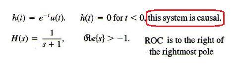
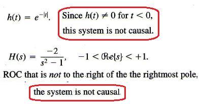
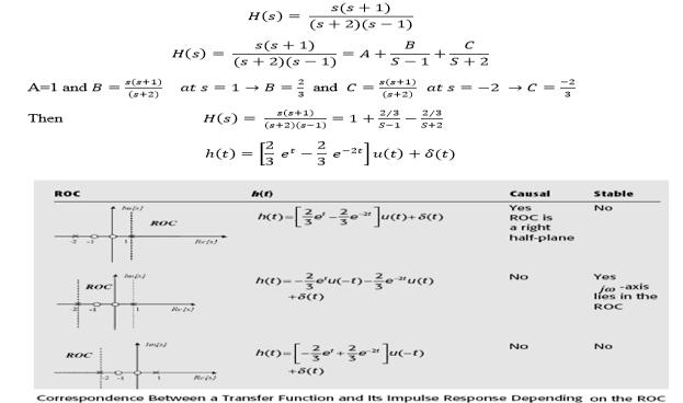
7 //7 Causality of TI Stability of TI 7

8 //7 s Hs s s a Res Causal, unstable system j j Transfer Function of the system TI Systems Characterized by inear Constant-Coefficient Differential Equations d y t N k M ak k k dt k k d x bk k dt t Y s H s X s M k N k k bk s ROC k a s k b - Res noncausal, stable system dyt 3yt xt dt c Res anticausal, unstable system j 9 3 Example Consider a causal TI system whose input and output related through an linear constant-coefficient differential equation of the form x t yt 3 y t y t y t x t Determine the unit step response of the system. t t s t e e u t H s s / C R / s / C 3 3 8

9 //7 Example 9.5 Consider an TI system with input x t e u, t 3t Output t t y t e e u t. (a) Determine the system function. (b) Justify the properties of the system. (c) Determine the differential equation of the system. s 3 H s Res - s s Example Consider a causal TI system, t t. xt e - t yt e - t 6 dht 4t. ht e ut but b unknown constant dt Hs Determine the system function and b. H s Res s s y t y t y t x t x t System Functions for Interconnections of TI Systems System Functions for Interconnections of TI Systems 9

10 //7 RC Circuit System Model Case RC Circuit System Model Case ( System Function & Impulse Response) RC Circuit System Model Case RC Circuit System Model Case ( System Function & Impulse Response) RC Circuit System Model Case

11 //7 Example: Example: Realization of Transfer Function Realization of Transfer Function First Order System

12 //7 Realization of Transfer Function Second Order System H s = s. +a s+a Realization of Transfer Function Second Order System H s = s. +a s+a Realization of Transfer Function Second Order System H s = s. +a s+a Realization of Transfer Function Second Order System H s = s. +a s+a

13 //7 Realization of Transfer Function Second Order System H s = s. +a s+a 3