Fundamentals of the gravitational wave data analysis V

Transcription

1 Fundamentals of the gravitational wave data analysis V - Hilbert-Huang Transform - Ken-ichi Oohara Niigata University

2 Introduction The Hilbert-Huang transform (HHT) l It is novel, adaptive approach to time series analysis proposed by Huang+ (1996) l It consists of Ø an empirical mode decomposition (EMD) Ø the Hilbert spectral analysis (HSA) l It can be applied to non-linear and non-stationary time series data l It has been applied to various fields; biomedical engineering, financial engineering, image processing, seismic studies, ocean engineering l I will review the method of the HHT and its application to search in GWs. 2

3 Contents l Hilbert Spectral Analysis (HSA) Ø Complex Signal (Analytic Signal) Ø Instantaneous Amplitude and Frequency (IA & IF) Ø Hilbert Transform Ø Problems in the simple HSA l Hilbert-Huang Transform Ø Empirical Mode Decomposition (EMD) and Intrinsic Mode Function (IMF) l Application of HHT to search for GWs Ø Results of Recent Research of Ours Ø Future Plans 3

4 Time-Frequency Analysis of GWs l GWs we will detect are mostly non-stationary. l Analysis of time-varying powers (or amplitudes) and frequencies in the time domain is important. l Traditionally for time-frequency analysis of GWs Ø the short-time Fourier transform (STFT) or Ø the wavelet analysis l The resolutions in time and frequency: restricted by "the uncertainty principle". l They require predetermined "window functions". 4

5 Demodulation I will discuss methods of high-resolution time-freq. analysis. A simple method of time-freq. analysis is demodulation. l Divide a signal h(t) into modulator and carrier: Ø modulator a(t) : a lower frequency signal Ø carrier c(t) or cosθ(t) : a higher frequency signal. l a(t): the time-varying amplitude or the instantaneous amplitude (IA) l θ(t): the phase h(t) = a(t)c(t) = a(t)cosθ(t) l the instantaneous frequency (IF) f (t) = 1 dθ(t) 2π dt 5

6 Complex Signals l The decomposition h(t) = a(t)c(t) is not unique. The problem will be better with a complex signal. l Assume h(t) = the real part of a certain complex function F(t) h(t) = Re F(t) ( ) or F(t) = h(t) + i v(t) = a(t)e iθ (t ) l a(t) = h(t) 2 + v(t) 2 : IA v(t) 1 dθ(t) θ(t) = tan 1 h(t) : the phase; f = 2π dt : IF l This is valid only if the time scale of varying a(t) is less than 1/f. 6

7 Hilbert Spectral Analysis (HSA) l How to find the complex signal F(t) or the imaginary part v(t) from h(t). l Hilbert Transform v(t) =H h(t) 1 π P h(t ') t t ' dt ' = h(t)* 1 πt P : the Cauchy's principal value * : the convolution l If h(t) is the real part on the real axis of a holomorphic function F(z) ( k>0, M>0, z k F(z) < M for z ), its imaginary part v(t) is uniquely given by the Hilbert transform of h(t). 7

8 How to calculate the Hilbert Transform l HT: convolution of h(t) and g(t)=1/πt; H h(t) = h(t)* 1 πt l FT of g(t)=1/πt : ĝ(ω ) = isgn(ω ) = i (ω > 0) 0 (ω > 0) i (ω > 0) l FT of H h(t): H h (ω ) = ĥ(ω )ĝ(ω ) where ĥ(ω ) is the FT of h(t) 8

9 How to calculate the Hilbert Transform l [ inverse FT of ĥ(ω )ĝ(ω )] = H h(r) l ĥ( ω ) = ĥ(ω )* since h(t) is real H h(t)= 1 2π = 1 2π ĥ(ω )ĝ(ω )e iωt dω 0 = i 2π 0 = Im 1 2π iĥ(ω )eiωt dω + ĥ(ω )e iωt 0 0 ĥ( ω )e iωt 2ĥ(ω )eiωt dω ( i)ĥ(ω )eiωt dω dω 9

10 How to calculate the Hilbert Transform H h(t)= Im 1 2π 0 2ĥ(ω )eiωt dω = Im 1 2π where h(ω ) = 2ĥ(ω ) (ω > 0) 0 (ω 0) h(ω )e iωt dω 1 h(t)= Re 2π 0 2ĥ(ω )eiωt dω = Re 1 2π h(ω )e iωt dω F(t) = h(t) + ih h(t) = 1 2π 2ĥ(ω )eiωt dω = 1 0 2π h(ω )e iωt dω 10

11 Examples of HT h(t) = sint cost exp(it) exp( it) 1 t 2 +1 sint t H h(t) = cost sint i exp(it) i exp( it) t t cost t H [ H h(t) ] = h(t) 11

12 Hilbert Transform l Consider h(t) = a(t) cosω 0 t, for example, where a(t) is slowly varying function of t, the Fourier components of a(t) vanish for ω >ω 0 l Its Hilbert transform: H h(t) = v(t) = a(t) sinω 0 t. l F(t) = h(t) + i v(t) = a(t) e iω 0 t l a(t) : the amplitude, f = ω 0 /2π: the frequency 12

13 The Chirp Signals l The chirp signals from the inspiral phase of CBC: h + (t) = A(τ ) 1+ cos2 ι cosφ(τ ) 2 h (t) = A(τ )cosιsinφ(τ ) where ι is the inclination of the orbital plane and A(τ ) = 4 r GM c c 2 5/3 f gw (τ ) = 1 5 π 256τ 3/8 π f gw c GM c c 2 2/3 5/8 τ 0 Φ(τ ) = 2π f gw (τ )dτ = Φ 0 2 τ τ = t coal t; 5GM c c 2 t coal : time at coalescence 5/8 τ 5/8 13

14 The Chirp Signals h + (t) = A(τ ) 1+ cos2 ι cosφ(τ ) 2 h (t) = A(τ )cosιsinφ(τ ) l Since A / A ~ τ 2 / f GW = P b (orbital period) in the inspiral phase, when τ = t coal t P b, we can consider A(τ ) 1+ cos2 ι and A(τ )cosι as the 2 amplitude of h + and h x and f GW as the frequency. 14

15 The Complex Chirp Signal l We cannot measure A(τ ) 1+ cos2 ι or A(τ )cosι 2 and cosφ(τ ) or sinφ(τ ) separately. l The output of the detector is h(t) = F + ( ˆn)h + (t) + F ( ˆn)h (t) F + ( ˆn) and F ( ˆn) ˆn : the detector pattern functions : the direction of propagation of the wave l Define the complex signal h(t) = F + ( ˆn) i F ( ˆn) as ( )( h + (t) + i h (t)) 1+ cos 2 ι = F + i F cosι 2 h(t) ( ˆF + i ˆF ) A(τ )( cosφ(τ ) + isinφ(τ )) A(τ ) ( cosφ(τ ) + isinφ(τ ) ) = h(t) + i v(t) 15

16 The Complex Chirp Signal l h(t) = ( ˆF + i ˆF ) A(τ )( cosφ(τ ) + isinφ(τ )) = ˆF+ 2 + ˆF 2 e iφ A(τ )e iφ(τ ) = ˆF+ 2 + ˆF 2 i Φ(τ )+φ A(τ )e ( ) ˆΦ(t Â(t)ei ) l IF: l IA: f GW (t) = 1 d ˆΦ(t) 2π dt h(t) = Â(t) = ˆF+ 2 + ˆF 2 A(τ ) 1+ cos ˆF 2 ι + = F +, ˆF = F cosι 2 16

17 The Complex Chirp Signal l l l IA: h(t) = Â(t) = ˆF+ 2 + ˆF 1+ cos 2 ι 2 A(τ ) ; ˆF+ = F +, ˆF = F cosι 2 detected by two or more detectors the position of the source is known F + and F are known h k (t) = ˆFk+ 2 + ˆF k 2 A(τ ); (k = 1, 2, ) h 1 (t) h 2 (t + Δt) = observed ˆF ˆF 2 1 ˆF ˆF 2 2 = F 1+ 2 F cos 2 ι 2 1+ cos 2 ι F 1 2 cosι + F 2 2 cosι cosι A(τ) 17

18 Time-frequency analysis of chirp signals l The time-frequency analysis can be made by the Hilbert spectral analysis (HSA) of observed chirp signals h(t); h(t) = F + ( ˆn)h + (t) + F ( ˆn)h (t) l The HSA is applied to the GWs from other phases of CBC, merger and ring-down phase, or other sources including continuous and burst sources. 18

19 HSA vs FSA l h(t) = cosω 1 t + cosω 2 t l The Fourier spectral analysis (FSA): superposition (or interference) of two waves of frequencies ω 1 and ω 2. 19

20 HSA vs FSA l h(t) = cosω 1 t + cosω 2 t l The Fourier spectral analysis (FSA): superposition (or interference) of two waves of frequencies ω 1 and ω 2. l The Hilbert spectral analysis (HSA) : beat 20

21 HSA vs FSA l h(t) = cosω 1 t + cosω 2 t l The Fourier spectral analysis (FSA): superposition (or interference) of two waves of frequencies ω 1 and ω 2. l The Hilbert spectral analysis (HSA) : beat h(t) = 2cos (ω ω )t 1 2 of frequency 2 with cos (ω + ω )t a modulated amplitude (ω 1 + ω 2 ) / 2 a(t) = 2cos (ω 1 ω 2 )t 2 = 2( 1+ cos(ω 1 ω 2 )) 21

22 22

23 Beat h(t) = a 1 cosω 1 + a 2 cosω 2 l ω 1 ω 2 ω 1 + ω 2 l Otherwise a beat superposition of two waves 23

24 a 1 = 1.0, ω 1 / 2π = 10Hz, a 2 = 0.5, ω 1 / 2π = 11Hz a 1 = 1.0, ω 1 / 2π = 3Hz, a 2 = 0.5, ω 1 / 2π = 10Hz 24

25 Beat h(t) = a 1 cosω 1 + a 2 cosω 2 l ω 1 ω 2 ω 1 + ω 2 l Otherwise a beat superposition of two waves l FSA HSA superposition beat (or sometime unphysical as the next discussion) l Question: Ø Is it possible to distinguish a beat or superposition depending on ω 1 ω 2? l Answer: 25

26 Problems in HSA l The IF is obtained as long as the integral h(t ') t t ' dt ' converges. l IF: not always physically meaningful l h(t) = a cosωt + b H h(t) = asinωt F(t) = h(t) + ih h(t) = ae iωt + b = A(t)e iφ(t ) IA: A(t) = ( a 2 + b 2 + 2abcosωt) 1/2 IF: f (t) = 1 dφ(t) 2π dt = ω a(a + bcosωt) 2π a 2 + b 2 + 2abcosωt 26

27 h(t) = cos2π f t + b, f = 5Hz b = 1.5 b = 0.75 b = 0 27

28 h(t) = cos2π f t + b, f = 5Hz F(t) = h(t) + ih h(t) = A(t)e iφ(t ) b = 0 b = 0.75 b = 1.5 phase diagram 28

29 h(t) = cos2π f t + b, f = 5Hz, b = 0 phase diagram The point of the complex signal moves along the circle at a constant speed in the complex plain. The phase increases with time at a constant rate and the frequency is constant. The amplitude is constant, too. 29

30 h(t) = cos2π f t + b, f = 5Hz F(t) = h(t) + ih h(t) = A(t)e iφ(t ) b = 0 b = 0.75 b = 1.5 phase diagram 30

31 h(t) = cos2π f t + b, f = 5Hz, b = 0.75 phase diagram The point moves at a constant speed. The phase increases monotonically But the rate changes with time; the frequency is not constant. The amplitude varies with time, too. It is not the case that the amplitude varies slowly. 31

32 h(t) = cos2π f t + b, f = 5Hz F(t) = h(t) + ih h(t) = A(t)e iφ(t ) b = 0 b = 0.75 b = 1.5 phase diagram 32

33 h(t) = cos2π f t + b, f = 5Hz, b = 1.5 phase diagram The phase decrease in some region. It causes a negative frequency. 33

34 Decomposition of Signals To overcome this problem and resolve the beat-or-superposition problem, l we need to decompose signal h(t) into some waves c k (t) and the non-wave part r(t); h(t) = c k (t) + r(t) = a k (t)cosφ k (t) + r(t) k k c k (t): intrinsic mode functions (IMF) r(t) : the trend (non-wave part) l a k (t) and r(t) are slowly varying functions. 34

35 Intrinsic Mode Functions (IMFs) l An IMF must satisfies the following conditions to obtain a meaningful IF: Ø oscillate around zero; in the whole data set, # of extrema # of zero = 0 or 1 Ø locally symmetric wrt zero; the mean value of the upper and lower envelopes defined by the local maxima and minima = 0 l Empirical Mode Decomposition (EMD): a sift procedure for decomposing a signal into IMFs. 35

36 Empirical Mode Decomposition (EMD) l l l Set h 1 (t) = h(t) (the original signal) for i = 1 to i max Ø h i1 (t) = h i (t) Ø for k = 1 to k max 1) Mark the local maxima and minima of h ik (t). 2) Interpolate the maxima and minima by cubic splines the upper U ik (t) and lower L ik (t) envelopes. 3) m ik (t) = (U ik (t) + L ik (t))/2. 4) h i,k+1 (t) = h ik (t) - m ik (t). Ø Exit if a certain stoppage criterion is satisfied. Ø IMF i is obtained; c i (t) = h ik (t). Ø Set h i+1 (t) = h i (t) - c i (t). Set the final residual r(t) = h imax+1 (t). 36

37 IMF1, iteration 0 l The original signal h 11 (t) = h 1 (t) = h(t) 37

38 IMF1, iteration 1 l Mark the maxima. 38

39 IMF1, iteration 1 l Interpolate the maxima by cubic splines to obtain the upper envelope U 11 (t). 39

40 IMF1, iteration 1 l Repeat the procedure to obtain the lower envelope L 11 (t). 40

41 IMF1, iteration 1 l Calculate the local mean curve m 11 (t) = (U 11 (t)+l 11 (t))/2. 41

42 IMF1, iteration 1 l Subtract the mean m 11 (t) from the original signal h 11 (t), 42

43 IMF1, iteration 2 l to obtain the residual h 12 (t) = h 11 (t) - m 11 (t). 43

44 IMF1, iteration 2 l Iterate the procedure on h 12 (t). l Mark the maxima and the minima. 44

45 IMF1, iteration 2 l Interpolate the maxima and minima to obtain the upper and lower envelopes, U 12 (t) and L 12 (t). l Calculate the local mean curve m 12 (t) = (U 12 (t)+l 12 (t))/2. l Subtract m 12 (t) from h 12 (t). 45

46 IMF1, iteration 3 l to obtain the residual h 13 (t) = h 12 (t) m 12 (t). 46

47 IMF1, iteration 3 l Iterate the procedure on h 1k (t), 47

48 IMF1, iteration 4 48

49 IMF1, iteration 4 49

50 IMF1, iteration 5 50

51 IMF1, iteration 6 51

52 IMF1, iteration 6 l until the stoppage criterion is satisfied; m 1k (t) is sufficiently small and/or the numbers of zero crossing and extrema of the residual h 1,k+1 (t) are equal or differ at most one. 52

53 IMF1 l Adopt h 1,k+1 (t) as IMF1, c 1 (t), if the stoppage criterion is satisfied. 53

54 IMF2, iteration 0 l Subtract IMF1 c 1 (t) from the original signal h 1 (t), 54

55 IMF2, iteration 1 l to obtain the residual h 2 (t) = h 1 (t) c 1 (t). l Apply the sifting process on h 2 (t) again to obtain IMF2. 55

56 IMF2, iteration 1 l Calculate the upper U 21 (t) and lower L 21 (t) envelops and the mean curve m 21 (t). l Subtract m 21 (t) from h 21 (t), 56

57 IMF2, iteration 2 l to obtain h 22 (t). 57

58 IMF2, iteration 2 l Iterate the procedure until the stoppage criterion is satisfied, 58

59 IMF2, iteration 3 59

60 IMF2 l and IMF2 is obtained. 60

61 IMF3 IMF4 l The sifting process is applies repeatedly to obtain IMF3, IMF4, etc. 61

62 residual l The sifting is completed when residual r(t) is smaller than the predetermined value, or when r(t) has at most one extremum. 62

63 the original signal h(t) IMF1 c 1 (t) Finally, the original signal is decomposed in terms of IMFs. h(t) = n i=1 c i (t) + r(t) IMF2 c 2 (t) IMF3 c 3 (t) IMF4 c 4 (t) residual r(t) 63

64 Empirical Mode Decomposition (EMD) l The EMD serves two purposes. Ø To decompose the signal into some waves of considerably different frequencies. Ø To eliminate the background trend on which the IMF is riding. Ø To make the wave profiles more symmetric. 64

65 Intrinsic Mode Functions (IMFs) v the first IMF: the finest-scale or the shortest-period oscillation v the next IMF: the next shortest-period one. l The EMD is a series of high-pass filters. l the residual r(t): Ø an oscillation of very long period or a signal varying monotonically Ø the adaptive local median or trend. 65

66 Stoppage Criteria of the EMD Several different types of stoppage criteria l the Cauchy type of convergence test (Huang et al 1998); the iteration is completed if m ik (t) is small enough, m ik (t j ) 2 < ε h ik (t j ) 2, j=1 with a predetermined value of ε. Ø mathematically rigorous N Ø not easy to predetermine the value of ε. N j=1 66

67 Stoppage Criteria of the EMD Another type of criterion proposed by Huang+ (1999, 2003) l the S stoppage; The EMD stops only after the numbers of zero crossing and extrema are: Ø Equal or differ at most by one. Ø Stay the same for S consecutive times. l the optimal range for S : between 3 and 8 (Huang et al 2003) l Any selection is ad hoc, and the optimal values of ε and S are likely to depend on the signal. 67

68 Hilbert-Huang Transform l Hilbert-Huang Transform (HHT) HSA of IMF time-frequency analysis of signals l The EMD: an adaptive decomposition Ø not require an a priori functional basis Ø the basis functions: adaptively derived from the data by the EMD sift procedure, instead l The HHT can be applied to nonlinear and non-stationary data. 68

69 Application of HHT to search for GWs l output of GW detectors: signal s(t) + noise n(t) h(t) = s(t) + n(t) l noise: spreading across broad band in the frequency domain l EMD decomposing the output into the signal and the noise 69

70 Problems with EMD l the original EMD: sensitive to noise Ø In the original form of the EMD, mode mixing frequently appears. l mode mixing Ø A single IMF consists of signals of widely disparate scale. Ø Signals of a similar scale reside in different IMF components. serious aliasing in the time-frequency distribution not physical meaningful IMF 70

71 Mode Mixing l Mode mixing often occurs if envelopes are close together and at height away from zero. 71

72 Ensemble EMD l Solution: Ensemble EMD (EEMD) Ø Proposed by Huang et al. (2009) Ø Inspired by the study of white noise using EMD l Algorithm: 1) Add white noise to the original data to form a "trial", h i (t) = h(t) + n i (t). 2) Perform EMD on each h i (t) with different n i (t). 3) For each IMF, take ensemble mean among the trials ( i = 1, 2, ) as the final answer. 72

73 EEMD l EEMD is a noise-assisted data analysis. l Noises act as the reference scale. They perturb the data in the solution space. l A noise contaminates the data. l Noises will be cancelled out ideally by averaging. 73

74 Parameters to be Predetermined l To perform the EMD or the EEMD, we must predetermine Ø stoppage criterion: the value of ε (the Cauchy type convergence) the number of S (the S stoppage) Ø the size of the ensemble for EEMD Ø the magnitude large noise to be added for EEMD 74

75 Application of HHT to search for GWs l In order to demonstrate applicability of the HHT to search for GWs, especially burst waves, and in order to determine optimal parameters of the EMD or the EEMD, we made simulations. (H. Takahashi+, Advances in Adaptive Data Analysis Vol5 (2013), ) 75

76 Setup for Simulation s(t) = a SG exp t /τ a SG : a constant to be fixed as SNR is specified l a sine-gaussian signals: τ = 0.016s Ø SG with constant freq. (SG-CF): ( ) 2 sinφ(t) φ(t) = 6π t 0.01s, f SG = 1 dφ 2π dt = 300Hz Ø SG with time-dependent frequency (SG-chirp) φ(t) = 2π 3 f SG = t 0.01s t 0.01s Hz t 0.01s 2, 76

77 Setup for Simulation l data to analyze: add noise to each signal h(t) = s(t) + n(t) l noise n(t): Gaussian noise of σ=1 l Signal-Noise Ratio (SNR): Ø SNR = 10 : Ø SNR = 20 : a SG = 1.56 a SG = 3.12 SNR = ( s(t j )) 2 j σ l how accurately the signal is recovered from the noisy data under the HHT with various parameters 77

78 Signal and Noise SG-CF Sine-Gaussian with Constant Freq. SG-chirp with Time-Dependent Freq. 78

79 Simulation l We performed the EMD and EEMD procedures for 400 samples of each data set; Ø injected signal: SG-CF and SG-chirp Ø SNR = 20 and 10 Ø stoppage criterion: S = 2, 4, 6; ε= 10-1, 10-2, 10-3, 10-4, 10-5, 10-6 Ø magnitude of the noise added for the EEMD σ e = 0.5, 1.0, 1.5, 2.0, 3.0, 5.0, 10.0, 20.0 Ø the size of the ensemble for the EEMD confirmed that the results change little with N e > 100 N e = 200; 79

80 IMFs: SG-CF, SNR=20 EMD EEMD 80

81 IMFs: SG-CF, SNR=10 EMD EEMD 81

82 IMFs: SG-chirp, SNR=20 EMD EEMD 82

83 IMFs: SG-chirp, SNR=10 EMD EEMD 83

84 Instantaneous Amplitudes (EEMD) Overlap of IAs of IMF2 4 for 30 samples with the EEMD SG-CF SG-Chirp 84

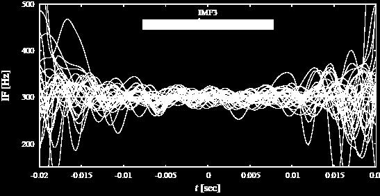
85 Instantaneous Frequencies (EEMD) Overlap of IFs of IMF3 for 30 samples with the EEMD SG-CF SG-Chirp 85

86 Regression for the IF l To determine the accuracy, the linear and quadratic regression are made for the IF f IMF (t) calculated with the HSA of each IMF. Ø the linear regression: f fit (t) = [ a 1 + b 1 (t / 0.01s) ]Hz Ø the quadratic regression: f fit (t) = a 2 + b 2 (t / 0.01s)+c 2 (t / 0.01s) 2 Hz n the exact values: a = 300, b = 0, c = 0 for SG-CF a = 300, b = 48, c = 0 for SG-chirp 86

87 Regression of IF (SG-CF) The coefficients of the linear and quadratic regression of IFs for SG-CF. The averages and the standard deviations of 400 samples are shown. The difference between EMD and EEMD is not apparent except for the quadratic regression of low SNR. 87

88 Regression of IF (SG-chirp) The coefficients of the linear and quadratic regression of IFs for SG-chirp. The averages and the standard deviations of 400 samples are shown. EMD gives worse results for low SNR, but difference between EMD and EEMD looks small for high SNR. 88

89 Indices of the Accuracy of Fitting l the relative error of fitting against the exact freq.: [ ] [ ] ρ = 100 WTSS f fit(t) f SG (t) WTSS f SG (t) the weighted total sum of squre: WTSS f (t) A(t) : the IA of the IMF [ ] A 2 (t j ) f 2 (t j ) j smaller ρ better fit to the exact freq. l the deviation of the IF for each IMF around the exact freq.: [ ] [ ] δ = 100 WTSS f IMF(t) f SG (t) WTSS f SG (t) It indicates how widely f IMF fluctuates around the exact freq. The procedure is considered unstable if δ is large, even if ρ is small. 89

90 Indices of the Accuracy of Fitting l the coefficient of determination: [ ] [ ] R 2 = 1 WTSS f fit(t) f IMF (t) WTSS f IMF (t) Ø R 2 is a measure of the goodness of fitting, too. Ø R 2 = 1 if the regression line perfectly fits the data; R 2 = 0 indicates no relationship between f IMF and t. Ø For SG-chirp (time-dependent freq.): R 2 1 indicates better fit Ø For SG-CF (constant freq.): R 2 0 indicates better fit 90

91 IF obtained with the EMD and EEMD The IFs with EMD fluctuate more widely than with EEMD. mode mixing 91

92 Comparison of σ e (SG-CF) the magnitude σ e of the noise added for the EEMD All except with very large σ e are acceptable. 92

93 Comparison of σ e (SG-chirp) the standard deviation σ e of the noise added for the EEMD All except with very large as well as small σ e are acceptable. 93

94 Plots of Coefficients for various σ e The dependence of the accuracy on σ e is rather weak. The best value of σ e depends on SNR; ~ 3.0 for SNR = 20; ~1.5 for SNR = 10 94

95 Comparison of stoppage criteria (SG-CF) All except with very small ε are acceptable. 95

96 Comparison of stoppage criteria (SG-chirp) Unstable with large ε. A rigid criterion is likely to cause the mode mixing. 96

97 Conclusion l The EMD tends to cause stronger mode mixing than the EEMD. l Stoppage criterion: the most important Ø The strict criterion is generally adequate. It sometimes causes mode mixing. It always requires long CPU time. Ø the optimal value: S = 2~4 or ε=10-4 l σ e : magnitude of the noise to be added for EEMD Ø The dependence on the accuracy is rather weak. Ø the optimal value: σ e = 1.0~3.0 (may depend on the amplitude of the signal) (H. Takahashi+, Advances in Adaptive Data Analysis Vol5 (2013), ) 97

98 Application of HHT to search in GWs Since HHT provides time-frequency analysis of waves Ø with fine resolution Ø without templates, it can be applied to l constructing a low-latency alert system for multi-messenger observation (M. Kaneyama, KO+ 2013) l detailed analysis of detected GWs from various sources including CBC, bursts of stellar core collapse (M. Kaneyama+ in collaboration with NR group, in preparation) l examining detector characterization (detchar) l 98