Numerical Simulation of Three-Phase Flows in the Inverse Fluidized bed

Transcription

1 Western University Electronic Thesis and Dissertation Repository October 2018 Numerical Simulation of Three-Phase Flows in the Inverse Fluidized bed Yunfeng Liu The University of Western Ontario Supervisor Zhang, Chao The University of Western Ontario Co-Supervisor Zhu, JingXu The University of Western Ontario Graduate Program in Mechanical and Materials Engineering A thesis submitted in partial fulfillment of the requirements for the degree in Master of Engineering Science Yunfeng Liu 2018 Follow this and additional works at: Part of the Mechanical Engineering Commons Recommended Citation Liu, Yunfeng, "Numerical Simulation of Three-Phase Flows in the Inverse Fluidized bed" (2018). Electronic Thesis and Dissertation Repository This Dissertation/Thesis is brought to you for free and open access by Scholarship@Western. It has been accepted for inclusion in Electronic Thesis and Dissertation Repository by an authorized administrator of Scholarship@Western. For more information, please contact tadam@uwo.ca, wlswadmin@uwo.ca.

2 Abstract The inverse three-phase fluidized bed has excellent potentials to be used in chemical, biochemical, petrochemical and food industries because of its high contact efficiency among each phase which leads to a good mass and heat transfer. The understanding of the hydrodynamics and flow structures in inverse three-phase fluidized beds is important for the design and scale up purposes. A CFD model based on the Eulerian-Eulerian (E-E) approach coupled with the kinetic theory of the granular flow is successfully developed to simulate an inverse three-phase fluidization system. The proposed CFD model for the inverse three-phase fluidization system is validated by comparing the numerical results with the experimental data. Investigations on the hydrodynamics and flow structures in the inverse three-phase fluidized bed under a batch liquid mode are conducted by numerical studies. The development of the fluidization processes and the general gas-liquid-solids flow structures under different operating conditions are further studied by the proposed three-phase E-E CFD model. Parametric studies including different inlet superficial gas velocities, particle densities, and solids loadings are investigated numerically. The numerical results show a general non-uniform radial flow structure in the inverse three-phase fluidized bed. It is also found that the particle distribution profiles in the axial direction relate to the solids loading, particle density and inlet superficial gas velocity. The existences of the liquid and solids recirculation inside the inverse three-phase fluidized bed are also noticed under the batch liquid mode. Moreover, the proposed CFD model for the inverse three-phase fluidized bed is further modified by adjusting the bubble size. The modified CFD model takes the bubble size effects into account and performs better on estimating the average gas holdup. In addition, a correlation between the bubble size and the superficial gas velocity, gas holdup and physical properties of the liquid and solid phases is proposed based on the numerical results. The predicted bubble size and the gas holdup in the inverse three-phase fluidized beds under a batch mode using the proposed correlation agree well with the experimental data. Therefore, the proposed three-phase E-E CFD model incorporated with the bubble i

3 size adjustment can be used to predict the performance of the inverse three-phase fluidization system more accurately. Keywords: computational fluid dynamic (CFD), inverse fluidized bed, three-phase flow, bubble size ii

4 Co-Authorship Statement Chapter 3 and Chapter 4 of this thesis will be submitted for publications. All papers are drafted by Yunfeng Liu and modified under the supervision of Prof. Chao Zhang and Prof. Jesse Zhu and in consultation with Miss Zeneng Sun in Prof. Chao Zhang s research group iii

5 Acknowledgement I would like to take this opportunity to express the gratitude and appreciation to those who have always been helping and supporting me throughout my master s study. First, I would like to express my sincerest thank to my Supervisor Prof. Zhu and Prof. Zhang, for believing my potential, providing me advice, support and encouragement through my entire research work. I attribute the thesis to their guidance and efforts, which ensured the work to be successfully completed. Then I would like to thank all members of our Computational Fluid Dynamics Research Laboratory, especially Zeneng Sun, Huirui Han, Hao Luo for their help and friendship in both academic and daily life. Finally, I would like to thank my parents for their encouragement and support during the entire process. iv

6 Table of Contents Abstract... i Co-Authorship Statement... iii Acknowledgement... iv Table of Contents... v Nomenclature... ix List of Tables... xi List of Figures... xii Chapter Introduction Background Literature review Experimental studies of the hydrodynamic characteristics of the inverse three-phase fluidized beds Modes of operation and flow regimes Particle movements Phase holdups Remarks CFD modelling of multiphase flows in fluidized beds Objectives v

7 1.4 Thesis structure Reference Chapter A CFD Model for the Simulation of the Inverse Gas-Liquid-Solid Fluidized Bed Introduction Experimental setup of the inverse three-phase fluidized bed Numerical models Governing equations Interphase forces Turbulence model Numerical methodology Results and discussion Grid independence test and CFD model validation Flow development and flow structure in an inverse three-phase fluidized bed Initial fluidization stage Developing stage Fully developed stage Effects of the solids loading General flow structure vi

8 2.5.5 Recirculation Conclusions Reference Chapter Modification of the CFD Model Based on the Bubble Size Adjustment for the Inverse Three-phase Fluidized Bed Introduction Experimental setup of the inverse three-phase fluidized bed Numerical models Governing equations Interphase forces Turbulence model Numerical methodology Grid Independence test Results and discussion Bubble size adjustment under different Ug Mean bubble size correlation Conclusions Reference Chapter vii

9 4 Conclusions and Recommendations Conclusions Recommendations Curriculum Vitae viii

10 Nomenclature Notation C 1ε Turbulence constants, dimensionless C 2ε Turbulence constants, dimensionless C 3ε Turbulence constants, dimensionless C D Drag coefficient, dimensionless d p Mean particles diameter, m d b Mean bubble size, m D e Column diameter, m Restitution coefficient for particle-particle collision, dimensionless ɡ Acceleration due to gravity, m/s 2 g 0 Radial distribution function, dimensionless G b Generation of turbulence kinetic energy due to buoyancy, m 2 /s 2 G k Generation of turbulence kinetic energy due to the mean velocity gradients, m 2 /s 2 H Column height from bottom to top, m k Turbulent kinetic energy, m 2 /s 2 K p Re t Interphase momentum exchange coefficient, kg/m 3 s Pressure, Pa Reynolds number, dimensionless Time, s ix

11 Ug Superficial gas velocity, m/s v x Velocity, m/s Radial position from left wall to right wall, m Greek letters α Local volume fraction, dimensionless ε Turbulent energy dissipation rate, m 2 /s 2 ε g Gas holdup, dimensionless γ Collision dissipation rate of energy, kg/ms 3 k Θs Granular conductivity, kg/m 3 s Θ Granular temperature, m 2 /s 2 λ μ Bulk viscosity, kg m/s Dynamic viscosity, kg/m-s ρ Density kg/m 3 τ Stress sensor, Pa Subscripts l g s Liquid phase Gas phase Solid phase x

12 List of Tables Table2.1 Operating conditions and physical properties of the liquid, gas and solid phases Table 2.2 Parameters of the RNG k-ɛ models Table 2.3 Mesh information for the grid independent test Table 2.4 Average gas holdups for different meshes Table 3.1 Operating conditions and physical properties of each phase Table 3.2 Parameters of the dispersed RNG k-ɛ models Table 3.3 Constitutive equations of the solid phases Table 3.4 Mesh information for the grid independent test Table 3.5 Average gas holdups from different meshes Table 3.6 Bubble sizes under the different inlet superficial gas velocities xi

13 List of Figures Figure 1.1 Schematic diagram of the gas-liquid-solid three-phase fluidization (Muroyama & Fan, 1985)... 4 Figure 1.2 Flow regimes in the three-phase inverse fluidized bed. (Fan et al., 1982)... 6 Figure 1.3 Flow regime map of the three-phase bubble column under the batch mode (Sun, 2017)... 7 Figure 2.1 Configuration of the experimental setup of the inverse three-phase fluidized bed (Sun, 2017) Figure 2.2 Computational domain of the inverse three-phase fluidized bed Figure 2.3 Comparison of the axial profiles of the solids volume fraction between the numerical results and experimental data at Ug=15 mm/s, 15% loading and ρs=930 kg/m Figure 2.4 Contours of the solids volume fraction at different time of the initial fluidization stage for Ug=15mm/s, 15% solids loading and ρs= 930 kg/m Figure 2.5 Axial profiles of the solids volume fraction at different time at the initial fluidization stage Figure 2.6 Radial profiles of the solids volume fraction at different axial locations at the initial fluidization stage (t=30s) Figure 2.7 Radial profiles of the gas volume fraction at different axial locations at the initial fluidization stage (t=30s) Figure 2.8 Radial profiles of the solids axial velocity at different axial locations at the initial fluidization stage (t=30s) Figure 2.9 Radial profiles of the liquid and gas axial velocities at H=0.5 m (t=30s) xii

14 Figure 2.10 Contours of the solids volume fraction at different time at the developing stage Figure 2.11 Axial profiles of the solids volume fraction at different time at the developing stage (t=150s) Figure 2.12 Radial profiles of the gas volume fraction at different axial locations at the developing stage (t=150s) Figure 2.13 Radial profiles of the solids volume fraction at different axial locations at the developing stage (t=150s) Figure 2.14 Radial profiles of the solids axial velocity component at different axial locations at the developing stage (t=150s) Figure 2.15 Contours of the solid phase volume fraction at the fully developed stage with time Figure 2.16 Time-averaged axial profile of the solids volume fraction at the fully developed stage Figure 2.17 Time-averaged axial profile of the gas volume fraction at the fully developed stage Figure 2.18 Time-averaged radial profiles of the solids axial velocity at different axial locations Figure 2.19 Time-averaged radial profiles of the solids volume fraction at different axial locations Figure 2.20 Time-averaged radial profiles of the solid and liquid axial velocities at H=1m Figure 2.21 Effects of the solids loading on the flow development time xiii

15 Figure 2.22 Axial profiles of the solids volume fraction under different solids loadings at Ug=15mm/s and ρs=930kg/m Figure 2.23 Radial profiles of the solids axial velocity under different solids loadings at Ug=15mm/s and ρs=930kg/m Figure 2.24 Radial profiles of the solids volume fraction under different solids loadings at Ug=15mm/s and ρs=930kg/m Figure 2.25 Radial profiles of the gas hold up at Ug=15mm/s and ρs=930kg/m Figure 2.26 Time required to reach to the developing and fully developed stages under differet inlet superficial gas velocities Figure 2.27 Contours of the solids volume fraction under different inlet superficial velocities at 15% solids loading and ρs=930 kg/m Figure 2.28 Radial profiles of the solids volume fraction under different inlet superficial gas velocities Figure 2.29 Average gas holdup under different particle densities at Ug=15mm/s, and 15% solids loading Figure 2.30 Contours of the solids volume fraction with different particle densities at 15% solids loading and Ug=15mm/s Figure 2.31 Radial profiles of solids holdup with different particle densities at 15% solids loading and Ug=15mm/s Figure 2.32 Radial profiles of the solids axial velocity under different inlet superficial gas velocities Figure 2.33 Instantaneous volume fraction contour (left) and particle velocity vector contour (right) xiv

16 Figure 3.1 Configuration of the experimental setup of the inverse three-phase fluidized bed (Sun, 2017) Figure 3.2 Computational domain of the inverse three-phase fluidized bed under the batch liquid mode Figure 3.3 Comparison of the average gas holdup between the numerical results and experimental data under the different inlet superfical gas velocities at 15% solids loading and ρs=930 kg/m Figure 3.4 Comparison of the axial gas holdups from the origin CFD model and modified CFD model with the experiment data at ρs=930 kg/m 3 and 15% solids loading Figure 3.5 Time-averaged radial gas holdups under different superficial gas velocities from the modified CFD model Figure 3.6 Comparison of the radial profiles of the gas holdup between the origin CFD model and the modified CFD model at 15% solids loading and ρs=930 kg/m xv

17 1 Chapter 1 1 Introduction 1.1 Background Fluidization is a process that makes the solid particles behave like fluid by introducing liquid or gas flow. The concept of the fluidized bed was first proposed for the gasification of coal in the 1920s, and the fluidization was used for fluid catalytic processes (FCC) in 1940s (Werther, Hartge, & Heinrich, 2014). Today, fluidized beds are widely used in chemical, biochemical, petrochemical and food industries because of the good heat and mass transfer. Usually, fluidized beds can be categorized by the fluidizing agent, so that there are liquidsolid two-phase fluidization, gas-solid two-phase fluidization and gas-liquid-solid (GLS) three-phase fluidization. Gas-solid fluidized beds were the first to be applied in industries, then the application extended to the liquid-solid and gas-liquid-solid fluidized beds. With the development of fluidization technology, fluidized beds can also be characterized by the flow directions after the concept of the inverse fluidized bed was proposed. Fluidized beds can be further divided into upward fluidized beds and inverse fluidized beds. For the traditional upward two-phase fluidization process, the liquid or gas is injected into the reactor from the bottom and flows through the space between particles. Under a low fluid velocity, the drag force acting on the particles cannot overcome the gravity of particles, causing them to remain packed. The fluidization begins as the fluid velocity reaches to the minimum fluidization velocity where the drag force acting on the particles can balance the gravity of the particles. Minimum fluidization velocity Umf is an important parameter for designing the fluidized bed (Zhu, Na, & Lu, 2007). By further increasing the fluid velocity, the drag force acting on particles will increase and particles will entrain out of the fluidized bed reactor, and the fluidized bed becomes a circulating fluidized bed if the entrained particles are recycled.

18 2 For gas-solid upward fluidization, the fluidized bed usually goes through the bubbling regime, turbulent regime, fast fluidization regime, to the pneumatic transport regime with the increase in the superficial gas velocity (Grace, 1986). For the gas-liquid-solid fluidization, the gas phase is usually introduced into the reactor as bubbles. The flow regime can be divided into dispersed bubble flow, discrete bubble flow, coalesced bubble flow, slug flow, churn flow, bridging flow and annular flow at different gas and liquid velocities (Zhang, Grace, Epstein, & Lim, 1997). As mentioned before, the three-phase GLS fluidized bed has been studied since 1970s with the development of fluidization technology (Ostergaard, 1971). Due to the close contact among solid, liquid and gas phases in GLS three-phase fluidized beds (TPFBs), it is used in chemical and biochemical processing (Muroyama & Fan, 1985). Three-phase fluidization can be divided into upward flow three-phase fluidization and inverse threephase fluidization depending on the flow direction of the gas and liquid phases. The different modes of three-phase fluidization is shown in Figure 1.1. Modes 1a and 1b are co-current flows where the air and liquid are injected from the bottom of the reactor and particles are moving upward. Modes 2a and 2b are countercurrent flows where the gas is introduced to the reactor from the bottom and the liquid is injected from the top of the reactor. The density of the particles used for modes 2a and 2b are usually less than the density of the liquid medium, allowing particles to overcome the buoyancy force and expand downward during the fluidization process. Besides modes 2a and 2b, the inverse fluidization can be also operated under the batch liquid mode (Comte, Bastoul, Hebrard, Roustan, & Lazarova, 1997; Sun, 2017), in which the liquid initially fills the reactor and the particles are floated at the top surface of the liquid before the operation starts. In the inverse fluidized bed under the batch mode operating condition, the fluidization state of the particles can be achieved with the zero liquid velocity when the superficial gas velocity is high enough resulting in the drag force and gravity acting on particles balanced with the buoyancy force. Compared to the upward flow three-phase fluidization, the inverse threephase fluidization can reduce energy cost and minimum solids attrition as the solid phase can be fluidized under low liquid and gas velocities, and the particle entrainment problem can be eliminated without using any external equipment (Ibrahim, Briens, Margaritis, & Bergongnou, 1996). The inverse three-phase fluidized bed has been started to be used in

19 3 wastewater treatment industries. Compared with the traditional methods of the wastewater treatment such as activated sludge process which requires longer retention time and large space, the retention time can be reduced in fluidized bed reactor due to high biomass concentration, and another problem of excessive growth of biomass on particles can be fixed by using light particles in inverse fluidized beds as well (Sokół & Korpal, 2006). Understanding the hydrodynamics of inverse three-phase fluidized beds is important when designing the reactors for industrial applications. Fan, Muroyama and Chern (1982) first defined the flow regime for the inverse three-phase fluidized bed, which are the fixed bed with dispersed bubble regime, bubbling fluidized bed regime, transition regime and slugging flow regime based on the liquid and gas velocities. Other flow characteristics in the inverse three-phase fluidized bed including the phase holdup, minimum fluidization velocity, pressure drop, bubble behavior, bed expansion has been studied by many researchers (Briens, Ibrahim, Margaritis, & Bergougnou, 1999; Renganathan & Krishnaiah, 2008; Son, Kang, Kim, Kang, & Kim, 2007). However, few researchers have reported the flow structure in the radial direction of the inverse three-phase fluidized bed. 1a 1b 2a 2b Diagram of GLS fluidized bed Continuous phase Liquid Gas Liquid Gas Flow direction Cocurrent Up-flow Countercurrent flow

20 4 Figure 1.1 Schematic diagram of the gas-liquid-solid three-phase fluidization (Muroyama & Fan, 1985) Although a few experimental studies on the hydrodynamics in GLS three-phase flows have been conducted, it is hard to fully understand the underlying phenomena of the GLS threephase fluidization due to the complex interactions between each phase. There is even less studies focused on predicting the flow characteristics of the inverse three-phase fluidized bed due to the restrictions of the experiments. Therefore, with the rapid development of computer technology, CFD has become a powerful tool to simulate the multiphase flow and provide more details on the three-phase fluidization process. In addition, CFD is considered to be more time and economic efficient to simulate complex flows compared with the experimental method. However, few CFD models has been developed to predict the hydrodynamics and flow structure in inverse three-phase fluidized beds (TPFBs). 1.2 Literature review The literature review will focus on two parts, which are the experiment studies on the hydrodynamics of the GLS three-phase inverse fluidized bed and the CFD simulations of the GLS three-phase fluidized bed Experimental studies of the hydrodynamic characteristics of the inverse three-phase fluidized beds Minimum fluidization velocity is an important parameter to consider when designing an inverse three-phase fluidized bed. Minimum fluidization velocity is defined as the velocity when the pressure gradient across the bed is minimum in the inverse three-phase fluidized bed (Ibrahim et al., 1996). Ibrahim et al.(1996) found that the minimum liquid fluidization velocity will decrease when increasing the gas velocity. Many researchers also reported the same trend in which the minimum liquid fluidization velocity decreases with the increase in gas flowrate (Bandaru, Murthy, & Krishnaiah, 2007; Cho, Park, Kim, Kang, & Kim, 2002; D. H. Lee, Epstein, & Grace, 2000; Renganathan & Krishnaiah, 2008). Renganathan and Krishnaiah (2008) also found the same results and developed the correlation for the minimum gas fluidization velocity in inverse three-phase fluidized beds under the batch liquid (Ul=0) operating condition.

21 Modes of operation and flow regimes Inverse three-phase fluidized beds can operate under the batch liquid mode or continuous mode. Under the batch liquid mode, the liquid velocity is zero, and the fluidization state of particles can be achieved by injecting gas only. The main method to determine the flow regime for inverse three-phase fluidized beds is by visual observation of the flow phenomena (particle movement or bubble behavior) in the experiment. Fan et al. (1982) conducted the first experimental study to investigate the hydrodynamics in the three-phase inverse fluidized bed. Both the gas and liquid phase can be considered as the continuous phase in an inverse three-phase fluidized bed. Fan et al. (1982) defined four flow regimes shown in Figure 1.2 based on the gas and liquid velocities in an inverse three-phase fluidized bed, which are: (a) the fixed bed with the dispersed bubble regime, (b) the bubbling fluidized bed regime, (c) the transition regime and (d) the slugging fluidized bed regime. In the fixed bed with dispersed bubble regime, the gas and liquid velocities are low, and the drag force and gravity acting on the particle cannot overcome the buoyancy force. In this regime, the particles remain packed. With the increase in gas and liquid velocities, the bubbling fluidized bed regime can be reached. The gravity and drag force exerted on particles can balance the buoyancy force, so, particles start to fluidize from the bottom of packed bed, ultimately distributing uniformly along the reactor. The bubble size is uniform within the bubbling fluidized bed regime. At the transition regime, bubbles starts to coalescence and their sizes will change. At the slugging fluidized bed regime, particles will move upward with slug bubbles, and then settle down quickly, and the interaction between particles and bubbles will affect their flows.

22 6 Figure 1.2 Flow regimes in the three-phase inverse fluidized bed. (Fan et al., 1982) Only a few researchers studied the batch mode of the inverse three-phase fluidized bed compared to the continuous mode. Comte et al. (1997) conducted experiments in an inverse TPFB under the batch mode operating condition. The particles used in the experiment have a mean density of 934 kg/m 3, and gas bubbles are introduced into the fluidized bed by using a perforate plate and membrane distributor. Three significant transition velocities have been defined based on different distributions of the solid phase to distinguish the flow regimes and study the flow behavior: (1) the minimum gas fluidization velocity Ug1 that can break the fixed bed; (2) velocity Ug2 is the velocity at which some particle can reach the bottom of the reactor; (3) velocity Ug3, at this velocity, the particle distribution is uniform along the reactor. It was found that Ug2 and Ug3 will decrease when increasing the solids loading or particle density. A mathematical model to predict velocity Ug3 was developed based on the assumption that the particle movement is mainly due to the density difference between particles and mixture of gas and liquid. Sun (2017) also proposed similar specific transition velocities, which are the initial fluidization velocity, expansion velocity, and complete fluidization velocity to study the flow behavior of solid phase

23 7 shown in Figure 1.3. In addition, when the superficial gas velocity is above Ug4, a free board region can be observed. It was also confirmed that Ug1, Ug2 and Ug3 will decrease with the increase in the particle density. Han et al. (2003) used particles with a density of 934 kg/m 3 but the gas distributor used in their experiment is different from the distributor used in the experimental study by Comte et al. (1997), so a different Ug3 value was derived. Thus, the gas distributor is one of the factors that can influence the Ug3 (Han et al., 2003). Sun (2017) further confirmed this fact by using particles with a density of 930 kg/m 3 and the porous quartz gas distributor, which can generate small bubbles, obtained the smallest Ug3 value among the three studies. Figure 1.3 Flow regime map of the three-phase bubble column under the batch mode (Sun, 2017) Particle movements Buffière and Moletta (1999) investigated the influence of the particle size and density on the flow regimes of the inverse fluidized bed under the batch liquid mode. Two types of particles are used in the experiment: one has a mean diameter of 4 mm with density of 920 kg/m 3 and the other one has a mean diameter of mm with a density of 690 kg/m 3.

24 8 For larger particles with a constant superficial liquid velocity, particles start to settle down and accumulate at the bottom of the reactor when the superficial gas velocity increases which results in a semi-fluidization phenomenon. For smaller particles, it was found that they will distribute uniformly in the reactor when the gas velocity is above a certain value, though the particle density is still smaller than the density of the surrounding liquid-gas mixture. In addition, smaller particles will flow upward with the liquid motion at a high gas velocity, so there is no semi-fluidization for smaller particles at a high gas velocity. In that case, two possible particle expansion mechanisms were proposed: (1) the density difference between particles and liquid-gas mixture and (2) the liquid circulation effect caused by rising bubbles. Later, Renganathan and Krishnaiah (2008) reported the particle expansion mechanism as a combination of the density difference effect and liquid circulation effect. It was indicated that the liquid circulation is not enough to cause the particle movement if the density difference between particles and the liquid-gas mixture is very large for large size particles Phase holdups Cho et al. (2002) conducted an experiment to find out the average phase holdup of an inverse TPFB under the continuous operating condition. The results showed the gas and liquid holdups will increase with an increase in the gas and liquid velocities. Later, Bandaru et al. (2007) also reported the same trend for the liquid average holdup. Only a few studies reported the axial distributions of flow parameters for each phase in inverse TPFBs. Ibrahim et al. (1996) and Bandaru et al. (2007) studied the distribution of the axial volume fraction of each phase in an inverse TPFB. It was found that the bed remains fixed at a lower gas and liquid velocity. With the increase in the inlet liquid or gas velocity, the packed bed starts to fluidize, and the particles begin to move downward. The gas phase holdup was eventually found to be uniform along the reactor. Buffière and Moletta (1999) proposed a correlation to predict the liquid holdup and bed porosity under the batch liquid mode in the inverse TPFB, and it can be used in the dispersed bubble regime and the transition regime. The gas holdup was found to be independent of the liquid velocity, and the gas holdup for large particles is higher than that of small particles under the same superficial gas velocity because the small particles may

25 9 not be able to break up the bubble. Sun (2017) reported that the gas holdup increases, and the liquid holdup decreases with a constant solids loading when increasing the superficial gas velocity. In addition, it was also reported that the local solids volume fraction in the axial direction decreases at the top and increases at the bottom of the column gradually with an increase in the superficial gas velocity Remarks Only a few researchers studied the fluidization process in inverse TPFBs. Most particles remain packed at the minimum fluidization velocity, and the hysteresis effect between the fluidization and defluidization was also found in inverse TPFBs (D. H. Lee et al., 2000). Renganathan and Krishnaiah (2008) observed that particles expanded layer by layer from the bottom of the packed bed instead of expanding suddenly at the minimum fluidization velocity under the batch liquid operating condition. The bed expansion was found to be heterogeneous first before reaching to the homogeneous expansion state (K. Il Lee et al., 2007). It was also found that the bed expands faster when using heavier particles or increasing gas and liquid velocities in inverse TPFBs. In an inverse TPFB, the gas is always introduced to the reactor as bubbles, which it is one of the key factors that can influence the heat and mass transfer. Therefore, it is important to study the bubble behavior and properties in order to better understand the flow characteristics of inverse TPFBs. Son et al. (2007) studied bubble properties in an inverse TPFB, and the results showed that the bubble size increases with an increase in the liquid or gas velocity. It was also found that the bubble size and the bubble rising velocity is higher when using the particles with smaller density. The correlation of bubble size, bubble rising velocity, and frequency was proposed based on the gas drift flux. Cho et al. (2002) also reported that the bubble size increases with an increase in the gas velocity CFD modelling of multiphase flows in fluidized beds In past decades, with the rapid development of the computer technology, computational fluid dynamics (CFD) has becomes a powerful tool to simulate multiphase flows as it is more time and economic efficient than experiments. There are two main approaches used

26 10 to simulate multiphase flows: (1) Eulerian-Eulerian approach and (2) Eulerian-Lagrangian approach. The Eulerian-Lagrangian approach treats the liquid and gas as a continuous phase by solving the Navier-Stokes equations, and the solid phase is treated as a discrete phase which can be solved by tracking the trajectories of each particle based on the Lagrangian force balance equation (ANSYS, 2014). Compared to the Eulerian-Eulerian approach, the advantages of the Eulerian-Lagrangian approach are that fewer empirical constitutive relations need to be used and the detailed information of the discrete phase can be obtained. Therefore, many researchers used the Eulerian-Lagrangian approach to investigate the flow characteristics of the discrete phase in micro-scales. Li, Zhang and Fan (1999) studied the single bubble wake behavior and particle entrainment phenomena in a GLS three-phase bubble column by using the VOF-DPM (volume of fluid-discrete phase model) which described the flows of gas bubbles and solid particles in the Lagrangian coordinates and the liquid phase in the Eulerian coordinates. Later, Zhang and Ahmadi (2005) developed a CFD model for the GLS slurry fluidized bed based on the Eulerian-Lagrangian method, and the effect of the bubble size on the flow structure and transient characteristics of the three-phase flows was studied. Wen, Lei and Huang (2005) treated the liquid and gas phases as continuous, and solid phase as the discrete phase to study the hydrodynamics in a TPFB and got a good agreement between the numerical results and experiment data. Since the Eulerian-Lagrangian approach tracks the trajectory of each individual particle, one of the fundamental assumptions made for the Eulerian-Lagrangian model is that the volume fraction of the discrete phase is low (ANSYS, 2014). The computational resource needed for simulating multiphase flows will be high if the discrete phase volume fraction is high (Pan, Chen, Liang, Zhu, & Luo, 2016). Although the Eulerian-Lagrangian method can predict the hydrodynamics of TPFBs accurately and provide more micro-scale information on the discrete phase, the Eulerian-Eulerian method will be used in the present work because the solids volume fraction in an inverse TPFB is high. The Eulerian-Eulerian approach treats all phases as the interpenetrating continuum, and all phases are solved using governing equations which are closed by additional closure laws and constitutive relations. A turbulence model is used as a closure law to solve the

27 11 governing equations for both the gas and liquid phases. Turbulence models used to close the Reynold-averaged Naiver Stokes can be divided into four categories: (1) zero-equation turbulence model; (2) one-equation turbulence model; (2) two-equation turbulence model and (4) RSM (Reynold Stress) turbulence model. The zero-equation turbulence model is the simplest eddy viscosity model that uses only one algebraic equation to calculate the turbulence viscosity. So, there are no other partial differential equations needed to calculate the turbulent stress. The Prandtl s mixing length theory was the first zero-equation turbulence model developed in 1920s (Prandtl, 1925) based on the Bounsinesq hypothesis (Boussinesq, 1877). But it only considered the mean velocity in a single direction. Later, Cebeci and Smith (1974) and Baldwin and Lomax (1978) extended the model to describe multi-dimensional turbulent flows. The drawbacks of the zero-equation turbulence model are the underestimation of the transport effects, and having difficulties in deriving the turbulence length scale for different types of flows from the empirical data. The one-equation turbulence model calculates the turbulent eddy viscosity by solving one more transport equation for the turbulent kinetic energy. Spallart and Allmaras (1992) developed a one-equation model, which can predict the free shear and boundary layer flows correctly. The advantage of the one-equation turbulence model is that less computation time is required. However, it also has the same drawback as the zero equation turbulence model in which the accuracy strongly depends on the specified turbulent length scale and time scale of the flow. Two-equation turbulence models such as the k model turbulence models are more popular than the zero and one-equation turbulence models because they overcome the drawbacks of the zero and one-equation models. The turbulent viscosity can be calculated by solving two additional transport equations for the turbulence kinetic energy and turbulence dissipation rate. Launder, Reece, and Rodi (1975) first developed the standard k turbulence model but it is only valid for high Reynolds number turbulent flows. To be used for low Reynold number flows, the wall function should be used with the standard k turbulence model in order to solve the flow in the near wall region correctly. Yakhot

28 12 and Orszag (1986) developed the RNG k model by adding addition terms and functions in the transport equation based on the renormalization group theory. Shih et al. (1995) developed the Realizable k model in order to improve the performance of the standard k model on predicting flows with a high shear rate and massive separation. The model has a new transport equation of dissipation rate related to the vorticity fluctuation at a high Reynolds number and a new formation for the turbulence viscosity based on realizability constraints. Laborde-Boutet et al. (2009) compared the performance of each turbulence models by predicting the turbulent flow characteristics in bubble columns. The results showed that the RNG k has a better performance than the standard and realizable k models. The study also investigated the influence of using different turbulence models, the dispersed k model, dispersed k model with bubble induce effect and per phase k model to account for the effect of the gas phase turbulence on the liquid phase turbulence. The results showed there is no influence on the predicted velocity filed, but the turbulent quantities are higher when accounting for the bubble induced turbulence. Masood and Delgado (2014) reported that both the dispersed RNG k model and dispersed RNG k model with bubble induced turbulence can predict the average velocity and turbulent accurately in a 3D square bubble column. Hamidipour, Chen, and Larachi (2012) extended the study to a three-phase bubble column and found the dispersed RNG k has a better performance on predicting the flow field in TPFBs bed than the per-phase RNG k model, realizable standard k model and standard k model. The RSM model is a second closure model, which closes governing equations by solving the transport equation of Reynold stresses instead of calculating the eddy viscosity. The RSM model has better performance on predicting the anisotropic flows than all other turbulence models mentioned above. The drawback of the RSM is the computation expense is high. Therefore, two equation turbulence models are used in the simulation of the multiphase fluidization in present work. For the solid phase, the kinetic theory of granular flow (KTGP) proposed by Chapman and Cowling (1970) is used to model the solid phase pressure, viscosity and stress in order to close the RANS equation. In the KTGP, the random motion of particles caused by particle-

29 13 particle collision can be analogous to the random motion of gas molecules in a thermodynamic system. The granular temperature is defined analogous to the temperature in a thermodynamic system, which is related the particle velocity fluctuation. The solids phase viscosity and stress are the functions of the granular temperature. Ding and Gidaspow (1990) modelled the gas-solid fluidization by using the KTGP. Later, some researchers also used the KTGP for the solid phase when modeling three-phase fluidization (Hamidipour et al., 2012; W. Li & Zhong, 2015; Wu & Gidaspow, 2000). Johnson and Jackson boundary condition (Johnson & Jackson, 1987) was often used for the solid phase to account for the collisions between the wall and particle, and the specularity coefficient is an empirical parameter to define the wall condition. The specularity coefficient can vary from zero to one where one represents the no-slip wall condition which means significant amount of lateral momentum transfer existed at wall, and zero represents the free-slip wall condition which means there is no shear at the wall. For the three-phase fluidization modelling, the Eulerian-Eulerian approach can be categorized into two types which are the pseudo two-fluid model and three-fluid Eulerian- Eulerian approach. The pseudo two-fluid model can be used for modeling the three-phase fluidization only when the gas bubble is smaller than the particle size and uniformly distributed along the column because the gas phase and fluid phase can be considered as a single mixed fluid phase (Felice, 2000). In addition, the two-fluid model is also applied to the three-phase fluidization when the particle size is small enough, the loading is low and the slip velocity between the solid and liquid phases is small. In that case, the liquid and solid suspension can be simplified to one-phase, and it is often used in the three-phase slurry bubble column simulation (Grevskott, Sannaes, Dudukovic, Hjarbo, & Svendsen, 1996; Hillmer & Weismantel, 1994; Wen & Xu, 1998). In addition, Feng et al. (2005) employed a pseudo two fluid model to the gas liquid-nanoparticles three-phase fluidization process, and the results was validated with the experimental data and the agreement was strong. By applying the pseudo two-fluid model for the three-phase simulation, the complicated three-phase flows can be simplified to a two-phase flow, which reduces the computation expanse as well. However, the drawback of the pseudo two-fluid model is that the application is limited by the particle size and particle loading, and it also neglects the interaction between the two phases. Therefore, the three-fluid Eulerian-

30 14 Eulerian approach will be used because of the large particle size used in the present study. Only a few literatures presented the CFD modelling based on the three-fluid Eulerian- Eulerian model as the interactions among each phase is complicated in TPFBs. Panneerselvam, Savithri, and Surender (2009) developed a CFD model for TPFBs based on the three-fluid Eulerian approach. Two different reactors were used to validate the model, and the particle densities are 2475 kg/m 3 and 2500 kg/m 3. The dispersed standard k turbulence model combined with the bubble and gas induced turbulence model on liquid was applied to the liquid phase. The constant viscosity model (Gidaspow, 1994) instead of the KTGP was used to describe the solid pressure and stress. Only the drag force was considered as the interaction force among each phase to calculate the momentum exchange coefficient. The drag model used between the liquid and solid phases is the Gidaspow drag model (Gidaspow, 1994). For the liquid and gas phases, the Tomiyama drag model (Tomiyama, 1998) and Grace drag models (Grace, 1973) were used, and the Tomiyama drag model gives a better performance by comparing the experimental results. The drag model used for the gas and particle phases in this study was the Schiller-Naumann drag model (Schiller & Naumann, 1935). The no-slip wall boundary condition for the liquid phase and free slip condition for the gas and solid phases were selected. The velocity inlet and pressure outlet were selected as boundary conditions. The mean bubble size is used without considering the bubble size distribution in their study (Panneerselvam et al., 2009), and it was determined by comparing the gas holdup derived from the CFD results using different bubble sizes with the average gas holdup from the experiment data. The simulation results showed a good agreement on the axial gas hold, axial solids velocity, and turbulence quantities such as turbulent velocity and shear stress with the experimental data. However, the model cannot predict the near wall region correctly. Hamidipour et al. (2012) presented a CFD model based on a three-fluid model combined with the KTGP in the same TPFBs as Panneerselvam et al. (2009) to investigate the performance of different turbulence models and solid wall conditions. A single bubble size distribution assumption was made in this study. The results showed the dispersed RNG k model gives a better performance on predicting the axial solids velocity and gas velocity than the other k models. According to this study, it was also found that both the three-

31 15 dimension and two-dimensional models are capable of predicting the flow field, but the three-dimensional model is slightly accurate than the two-dimensional model. However, the computational cost of the three- dimensional simulation is also high. The no-slip wall condition for the liquid phase, free-slip for the gas and solids phases were recommended. The bubble size input for the second phase was found to have an influence on the gas holdup, and the smaller bubble size resulted in a higher gas holdup. Also, the interphase force between the continuous and dispersed phases has been studied widely in literatures, but the interaction between two dispersed phases has not been well understand and modeled. Hamidipour et al. (2012) used the same method to model the drag force between the two dispersed phases to model the drag force between the continuous and dispersed phases because two dispersed phases were also treated as continuums in the Eulerian-Eulerian approach. The drag model used between the gas and solid phases was the Schiller- Naumann drag model (Schiller & Naumann, 1935), between the solid and liquid phase was the Gidaspow drag model (Gidaspow, 1994), between the liquid and gas phase was also the Schiller-Naumann model (Schiller & Naumann, 1935). Li and Zhong (2015) did the CFD modeling using the three-fluid Eulerian-Eulerian approach with the KTGP to investigate the hydrodynamics of the three-phase phase bubble columns. The dispersed RNG model was used for the liquid phase. A mean bubble size was applied even under different superficial gas velocities. The sensitivity of the interphase force, which includes the drag force, was studied. It was found the best drag model for the liquid and gas phases is the Zhang-Vanderheyden model (Zhang & Vanderheyden, 2002), between liquid and solid phases is the Schiller-Naumann drag model (Schiller & Naumann, 1935), and the drag force between the gas and solid phases were not considered. The effect of the superficial gas velocity, particle density, solids loading and particle size on the hydrodynamics of the three-phase bubble column is investigated based on the CFD results. According to literatures, very few works were focused on developing CFD model based on three-fluid Eulerian-Eulerian approach for the three-phase fluidization process, and most of the CFD models are for upward TPFBs. No CFD model for the inverse three-phase fluidization process with light particle has been reported in the literature. Only very few studies which relate to the CFD modeling of the hydrodynamics of inverse two-phase

32 16 fluidized bed has been reported. The following literature review is about liquid-solid inverse fluidized beds. A numerical simulation based on the Eulerian-Eulerian approach has been carried out to study the flow behavior of particles in the inverse liquid-solid fluidization process by Wang et al. (2014). The dispersed standard k turbulence model for the liquid phase and KTGP for the solid phase were applied. The Gidaspow drag model is used to determine the interphase momentum exchange coefficient. The no-slip wall condition was used for both the liquid and solid phases. The particle density was 897 kg/m3 which is lower than the surrounding liquid phase density. The predicted bed expansion was slightly higher than the experimental value. The effects of the liquid velocity on the bed height, solid phase distribution and flow patterns of particles were investigated. Further improvement of the drag model is needed to enhance the performance of CFD model in inverse liquid-solid fluidized beds. Wang et al. (2018) developed a CFD model for inverse liquid-solid fluidized beds based on the Eulerian-Larganrain approach. The effects of the particle velocity, jet velocity and liquid viscosity on the particle flow behavior was studied. The results indicated that the solid distribution was denser at the bottom of the column for heavily particles than light particles in an inverse liquid-solid fluidized bed. It was also found that a higher particles restitution coefficient will give a higher bed expansion height.

33 Objectives According to the literature review presented in the previous section, it is noticed that the hydrodynamics of the inverse fluidized bed has been studied experimentally by many researchers, but most studies were focused on the flow characteristics, such as the average phase holdup, axial phase holdup, and minimum fluidization velocity. However, few of them reported the details of the flow patterns and local flow characteristics such as local radial phase holdup, radial solid phase velocity and etc. In addition, few researchers investigated the development process of the inverse three-phase fluidization process. For CFD models, only a few models were developed and validated for the three-phase fluidization process based on the three-fluid Eulerian-Eulerian approach. The complicated interactions between each phase are still not well understood, and there is no clear guideline to follow when setting up a CFD model for the simulation of the three-phase fluidization process. In addition, there is no CFD model developed for inverse TPFBs from literatures. The mean bubble size is assumed to be constant even under different superficial gas or liquid velocities operating condition from literatures. However, in reality, the mean bubble size varies with the superficial gas velocity. The first objective of the present work is to develop a CFD model for the simulation of the inverse TPFB based on the three-fluid Eulerian-Eulerian approach in order to study the flow details and fluidization development process in the inverse TPFB, which have not been reported by experimental studies. The second objective is to further modify the proposed CFD model by using different mean bubble sizes under different inlet superficial gas velocities. In addition, a correlation between the bubble size and inlet superficial gas velocity in the inverse TPFB will be developed.

34 Thesis structure The thesis is in the Integrated-Article Format. Chapter1: General background and literature review on CFD modelling and experiment study of the three-phase fluidization process is presented. Chapter2: A CFD model is developed for the simulation of the inverse TPFB. The development of the fluidization process and the effect of the operating condition on the hydrodynamics and flow structure are investigated. Chapter3: The CFD model proposed in chapter 2 is modified based on the mean bubble size adjustment and the correlation for the bubble size. Chapter4: Conclusions and recommendations for future work are presented.

35 19 Reference Ansys. Inc. (2014). Fluent 16.0 User s Guide. Baldwin, B., & Lomax, H. (1978). Thin-layer approximation and algebraic model for separated turbulentflows. In 16th Aerospace Sciences Meeting. American Institute of Aeronautics and Astronautics. Bandaru, K. S. V. S. R., Murthy, D. V. S., & Krishnaiah, K. (2007). Some hydrodynamic aspects of 3-phase inverse fluidized bed. China Particuology, 5(5), Boussinesq, J. (1877). Essai sur la theorie des eaux courantes. Mémoires Présentés Par Divers Savants à l Acad. Des Sci. Inst. Nat. France, 23(1), Briens, C. L., Ibrahim, Y. A. A., Margaritis, A., & Bergougnou, M. A. (1999). Effect of coalescence inhibitors on the performance of three-phase inverse fluidized-bed columns. Chemical Engineering Science, 54(21), Buffière, P., & Moletta, R. (1999). Some hydrodynamic characteristics of inverse three phase fluidized-bed reactors. Chemical Engineering Science, 54(9), Cebeci, T., & Smith, A. M. O. (1974). Analysis of turbulent boundary layers. (A. M. O. Smith, Ed.). New York: Academic Press. Chapman, S., & Cowling, F. (1991). The Mathematical Theory of Non-uniform Gases An Account of the Kinetic Theory of Viscosity, Thermal Conduction and Diffusion in Gases. Cambridge University Press. Cho, Y. J., Park, H. Y., Kim, S. W., Kang, Y., & Kim, S. D. (2002). Heat transfer and hydrodynamics in two- and three-phase inverse fluidized beds. Industrial and Engineering Chemistry Research, 41(8), Comte, M. P., Bastoul, D., Hebrard, G., Roustan, M., & Lazarova, V. (1997). Hydrodynamics of a three-phase fluidized bed - The inverse turbulent bed. Chemical Engineering Science, 52(21 22), Ding, J., & Gidaspow, D. (1990). A bubbling fluidization model using kinetic theory of granular flow. AIChE Journal, 36(4), Fan, L. S., Muroyama, K., & Chern, S. H. (1982). Hydrodynamic characteristics of inverse fluidization in liquid-solid and gas-liquid-solid systems. The Chemical Engineering Journal, 24(2),

36 20 Felice, R. Di. (2000). The pseudo-fluid model applied to three-phase fluidisation. Chemical Engineering Science, 55(18), Feng, W., Wen, J., Fan, J., Yuan, Q., Jia, X., & Sun, Y. (2005). Local hydrodynamics of gas liquid-nanoparticles three-phase fluidization. Chemical Engineering Science, 60(24), Gidaspow, D. (1994). Multiphase Flow and Fluidization: Continuu and Kinetic Theory Descriptions. Boston: Acad. Press. Grace, J. R. (1973). Shapes and velocities of bubbles rising in infinite liquids. Transactions of the Institution of Chemical Engineers, 51, Retrieved from Grace, J. R. (1986). Contacting modes and behaviour classification of gas solid and other two phase suspensions. The Canadian Journal of Chemical Engineering, 64(3), Grevskott, S., Sannaes, B. H., Dudukovic, M. P., Hjarbo, K. W., & Svendsen, H. F. (1996). Liquid circulation, bubble size distributions, and solid movement in two- and threephase bubble columns. Chemical Engineering Science, 51(10), Hamidipour, M., Chen, J., & Larachi, F. (2012). CFD study on hydrodynamics in threephase fluidized beds Application of turbulence models and experimental validation. Chemical Engineering Science, 78, Han, H., Lee, W., Kim, Y., Kwon, J., Choi, H., Kang, Y., & Kim, S. (2003). Phase Holdup and Critical Fluidization Velocity in a Three-Phase Inverse Fluidized Bed. Korean J. Chem. Eng., 20(1), Hillmer, G., & Weismantel, L. (1994). Investigations and Modelling Columns of Slurry Bubble. Science, 49(6), Ibrahim, Y. A. A., Briens, C. L., Margaritis, A., & Bergongnou, M. A. (1996). Hydrodynamic Characteristics of a Three-Phase Inverse Fluidized-Bed Column. AIChE Journal, 42(7), Il Lee, K., Mo Son, S., Yeong Kim, U., Kang, Y., Hwan Kang, S., Done Kim, S., Hyun Kim, W. (2007). Particle dispersion in viscous three-phase inverse fluidized beds. Chemical Engineering Science, 62(24), Johnson, P. C., & Jackson, R. (1987). Frictional-collisional constitutive relations for granular materials, with application to plane shearing. Journal of Fluid Mechanics,

37 21 176, Laborde-Boutet, C., Larachi, F., Dromard, N., Delsart, O., & Schweich, D. (2009). CFD simulation of bubble column flows: Investigations on turbulence models in RANS approach. Chemical Engineering Science, 64(21), Launder, B. E., Reece, G. J., & Rodi, W. (1975). Progress in the development of a Reynolds-stress turbulence closure. Journal of Fluid Mechanics, 68(3), Lee, D. H., Epstein, N., & Grace, J. R. (2000). Hydrodynamic Transition from Fixed to Fully Fluidized Beds for Three-Phase Inverse Fluidization. Korean Journal of Chemical Engineering, 17(6), Li, W., & Zhong, W. (2015). CFD simulation of hydrodynamics of gas-liquid-solid threephase bubble column. Powder Technology, 286, Li, Y., Zhang, J., & Fan, L.-S. (1999). Numerical simulation of gas liquid solid fluidization systems using a combined CFD-VOF-DPM method: bubble wake behavior. Chemical Engineering Science, 54(21), Masood, R. M. A., & Delgado, A. (2014). Numerical investigation of the interphase forces and turbulence closure in 3D square bubble columns. Chemical Engineering Science, 108, Muroyama, K., & Fan, L. S. (1985). Fundamentals of gas liquid solid fluidization. AIChE Journal, 31(1), Ostergaard, K. (1971). Three-phase fluidization. In J. F. Davidson & D. Harrison (Eds.), Fluidization (pp ). Academic Press London. Pan, H., Chen, X., Liang, X., Zhu, L., & Luo, Z. (2016). CFD simulations of gas liquid solid flow in fluidized bed reactors A review. Powder Technology, 299, Panneerselvam, R., Savithri, S., & Surender, G. D. (2009). CFD simulation of hydrodynamics of gas liquid solid fluidised bed reactor. Chemical Engineering Science, 64(6), Prandtl, L. (1925). Uber die ausgebildete Turbulenz. Zamm, Vol. 5(5), Renganathan, T., & Krishnaiah, K. (2008). Prediction of Minimum Fluidization Velocity in Two and Three Phase Inverse Fluidized Beds. The Canadian Journal of Chemical Engineering, 81(3 4),

38 22 Schiller, L., & Naumann, A. (1935). A drag coefficient correlation. Z. Ver. Deutsch. Ing, 77, Shih, T.-H., Liou, W. W., Shabbir, A., Yang, Z., & Zhu, J. (1995). A new eddy viscosity model for high Reynolds number turbulent flows. Computers and Fluids, 24(3), Sokół, W., & Korpal, W. (2006). Aerobic treatment of wastewaters in the inverse fluidised bed biofilm reactor. Chemical Engineering Journal, 118(3), Son, S. M., Kang, S. H., Kim, U. Y., Kang, Y., & Kim, S. D. (2007). Bubble properties in three-phase inverse fluidized beds with viscous liquid medium. Chemical Engineering and Processing: Process Intensification, 46(8), SPALART, P., & ALLMARAS, S. (1992). A one-equation turbulence model for aerodynamic flows. In 30th Aerospace Sciences Meeting and Exhibit. American Institute of Aeronautics and Astronautics. Sun, X. (2017). Bubble induced Inverse Gas-liquid-solid Fluidized bed. University of Western Ontario. Tomiyama, A. (1998). Struggle with computational bubble dynamics. Multiphase Science and Technology. Wang, S., Li, H., Wang, R., Tian, R., Sun, Q., & Ma, Y. (2018). Numerical simulation of flow behavior of particles in a porous media based on CFD-DEM. Journal of Petroleum Science and Engineering, 171, Wang, S., Sun, J., Yang, Q., Zhao, Y., Gao, J., & Liu, Y. (2014). Numerical simulation of flow behavior of particles in an inverse liquid solid fluidized bed. Powder Technology, 261, Wen, J., Lei, P., & Huang, L. (2005). Modeling and simulation of gas-liquid-solid threephase fluidization. Chemical Engineering Communications, 192(7 9), Wen, J., & Xu, S. (1998). Local hydrodynamics in a gas-liquid-solid bubble column reactor. Science, 70(97), Werther, J., Hartge, E. U., & Heinrich, S. (2014). Fluidized-bed reactors-status and some development perspectives. Chem. Ing. Tech., 86(12),

39 23 Wu, Y., & Gidaspow, D. (2000). Hydrodynamic simulation of methanol synthesis in gasliquid slurry bubble column reactors. Chemical Engineering Science, 55(3), Yakhot, V., & Orszag, S. A. (1986). Renormalization group analysis of turbulence. I. Basic theory. Journal of Scientific Computing, 1(1), Zhang, D. Z., & Vanderheyden, W. B. (2002). The effects of mesoscale structures on the disperse two-phase flows and their closures for dilute suspensions. Int. J. Multiphase Flows, 28(5), Zhang, J. P., Grace, J. R., Epstein, N., & Lim, K. S. (1997). Flow regime identification in gas-liquid flow and three-phase fluidized beds. In Chemical Engineering Science (Vol. 52, pp ). Pergamon. Zhang, X., & Ahmadi, G. (2005). Eulerian Lagrangian simulations of liquid gas solid flows in three-phase slurry reactors. Chemical Engineering Science, 60(18), Zhu, Z., Na, Y., & Lu, Q. (2007). Effect of pressure on minimum fluidization velocity. Journal of Thermal Science, 16(3),

40 24 Chapter 2 2 A CFD Model for the Simulation of the Inverse Gas-Liquid- Solid Fluidized Bed 2.1 Introduction Fluidization is a process that can convert particle behavior from the solid state to a fluid state by introducing liquid or gas flow into the system. Fluidized beds can be categorized as the liquid-solid fluidization, gas-solid fluidization and gas-liquid-solid three-phase fluidization using different fluidizing agents. Due to the higher contact efficiency among each phase and good mass and heat transfer features, gas-liquid-solid three-phase fluidized beds (TPFBs) have the potential to be used in chemical, biochemical, and petrochemical industries since past decades (Muroyama & Fan, 1985). In addition, fluidized beds can be further divided into upward fluidized beds and inverse fluidized beds based on the flow direction of the fluidizing agent. The inverse gas-liquid-solid TPFBs can be operated under the continuous mode or batch mode. Under the batch mode, the liquid velocity is zero, and the fluidization state of the system can be achieved by increasing the gas velocity. In inverse TPFBs, the particle density is usually smaller than the liquid density, so fluidization will begin when the drag force and gravity of particles can balance with the buoyancy force when increasing the liquid or gas velocity. Comparing to the traditional upward three-phase fluidization, inverse three-phase fluidization possesses some advantages such as lower energy cost and minimum solids attrition. The hydrodynamics and flow patterns in inverse fluidized beds have been studied by a few researchers. The flow regimes in inverse fluidized beds are defined as the fixed bed with dispersed bubble regime, bubbling fluidized bed regime, transition regime and slugging fluidized bed regime with an increase in the liquid velocity or gas velocity (Fan et al., 1982). Three significant transition superficial gas velocities have been defined based on the solid phase distribution in the inverse fluidized bed under the batch liquid mode to distinguish the flow regimes, being (1) the minimum gas fluidization velocity (Ug1) that can break the fixed bed, (2) the velocity (Ug2) that can let some particles reach the bottom of the reactor, and (3) the velocity (Ug3) that can distribute particles uniformly along the reactor (Comte

41 25 et al., 1997; Sun, 2017). It was found that Ug2 and Ug3 will decrease when increasing the solids loading or particle density. A few researchers experimentally investigated the hydrodynamics, such as the minimum fluidization velocity and phase holdup in inverse TPFBs. The minimum liquid fluidization velocity decreased with an increase in the gas flowrate, and the gas and liquid holdup was found to increase with the increase in the gas and liquid velocities (Bandaru et al., 2007; Cho et al., 2002; D. H. Lee et al., 2000). Renganathan & Krishnaiah (2008) developed a correlation, which can predict the minimum fluidization velocity in the inverse TPFB under both the batch mode and continuous mode. The solids holdup was found to become denser at the lower part of the column and dilute at the upper part of the column when increasing the liquid or gas velocity, and the gas holdup is distributed uniformly along the axial direction of the column (Bandaru et al., 2007; Ibrahim et al., 1996; Sun, 2017). The solid phase expansion in the inverse TPFB is due to the combination of the density difference and liquid circulation, and it was also found particles are easier to be fluidized when their density is close to the gas-liquid mixture density (Buffière & Moletta, 1999). Despite a few experimental studies on the hydrodynamics and flow structure conducted, the understanding of the hydrodynamics of inverse TPFBs is still limited. For instance, no studies were found in the literatures that reported the hydrodynamics of an inverse TPFB in the radial direction. CFD has become a powerful tool to study the multi-phase flows in fluidized beds due to the rapid development of computer technology in past decades. Therefore, a numerical study on the hydrodynamics of an inverse fluidized bed will be conducted in the present study in order to better understand the flow patterns and hydrodynamics in the inverse TPFB under the batch mode. Two main methods are usually used to simulate flows in fluidized beds, which are the Eulerian-Lagrangian approach and Eulerian-Eulerian approach. In the Eulerian- Lagrangian approach, the liquid phase is treated as the continuous phase and the solid phase is treated as the discrete phase in which each individual particle is tracked by solving the Lagrangian force balance equation. The Eulerian-Lagrangian approach is typically used when the volume fraction of the discrete phase is low to study the single bubble and particle

42 26 behavior in the TPFB (Y. Li et al., 1999). When the volume fraction of the discrete phase is high, the Eulerian-Eulerian approach is preferred. Therefore, the Eulerian-Eulerian approach will be used in present study since the volume fraction of particles in an inverse three-phase fluidized bed is high. The Eulerian-Eulerian approach treats all phases as an interpenetrating continuum, and the governing equations are solved for each phase with additional closure law and constative relations. The kinetic theory of the granular flow (Ding & Gidaspow, 1990; Hamidipour et al., 2012; W. Li & Zhong, 2015; Wu & Gidaspow, 2000) is used to calculate the solid phase pressure, viscosity and stress. The Eulerian-Eulerian approach can be divided into the pseudo two-fluid Eulerian model and three-fluid Eulerian-Eulerian model for the threephase flows. For the pseudo two-fluid Eulerian model, the liquid-solid or liquid-gas can be treated as one mixed phase when the particle or bubble size is small, volume fraction of the solid or gas phase is low and the slip velocity between the two phases is low. Therefore, the three-phase flows can be simplified to a two-phase flows, which is often used to simulate the flow in the three-phase slurry fluidized bed or the fluidized bed that used nanoparticles as solid phase (Feng et al., 2005; Grevskott et al., 1996; Hillmer & Weismantel, 1994; Wen & Xu, 1998). Due to the limitation of the pseudo two-fluid model, the three-fluid Eulerian-Eulerian model is used in present study to simulate the three-phase flows in a fluidized bed under the batch operating mode. Comparing to the traditional upward two-phase flows in fluidized beds, fewer researchers have been done the numerical study on hydrodynamics in TPFBs. Panneerselvam et al. (2009) developed a CFD model to simulate gas-liquid-solid fluidized beds based on the three-fluid Eulerian-Eulerian approach, and the results shows a good agreement with the experimental data except at the near wall region. Hamidipour et al. (2012) presented a CFD model based on the three-fluid Eulerian-Eulerian approach and kinetic theory of the granular flow to investigate the performance of different turbulence models and wall boundary conditions for the solid phase. It was found the dispersed RNG k model has the best performance. Li and Zhong (2015) studied the performance of different drag models in TPFBs. It was found the best drag model for the liquid and gas phases is the Zhang-Vanderheyden model (Zhang & Vanderheyden, 2002), between the liquid and solid

43 27 phases is the Schiller-Naumann drag model (Schiller & Naumann, 1935), and the drag force between the gas and solid phases were not considered. No CFD studies on inverse TPFBs were found in the literatures. Therefore, the objective of this study is to develop a CFD model based on the three-fluid Eulerian-Eulerian approach with the kinetic theory of the granular flow for an inverse TPFB in order to better understand the hydrodynamics and flow patterns within it. 2.2 Experimental setup of the inverse three-phase fluidized bed The proposed CFD model will be validated based on the he experimental work done by Sun (2017). The schematic diagram of the experiment set up is shown in Figure 2.1. The column is made of PVC with m in diameter and 3 m in height. The ring-shape porous quartz gas distributor with an 8.7 cm outer diameter and a 2.7 cm inner diameter which can generate very small bubbles, is placed at the bottom of the column. The tap water, air and particles are used as the liquid, gas and solid phases, respectively, in the experiment. Three types of particles with different densities (904 kg/m 3, 930 kg/m 3 and 950 kg/m 3 ) are used. Before the experiment begins, tap water and particles are injected into the column. The particles rise to the surface as the particle density is lower than the liquid density. During the experiment, only the gas is continuously introduced into the column through the gas distributor, and there are no inlets and outlets for particles and liquid. The superficial velocity of the gas at the inlet is from 0mm/s to 60mm/s. The experiment is carried out under ambient temperature and pressure. In this study, the simulation of the three-phase flows in the inverse TPFB will be carried out under different operating conditions, such as different particle densities, inlet superficial gas velocities, and solids loadings, in order to study the hydrodynamics and flow structures in the inverse TPFB. The summary of the operating conditions and properties of each phase are shown in Table 2.1.

44 28 1 Column 2 Bubble 3 Liquid 4 Solid particles 5 Rotameters 6 Pressure gauge 7 Gas distributor 8 Liquid inlet/outlet valve 9 Manometer Figure 2.1 Configuration of the experimental setup of the inverse three-phase fluidized bed (Sun, 2017)

45 29 Table2.1 Operating conditions and physical properties of the liquid, gas and solid phases Bubble column size (m) Diameter: Total height: 3 U l (mm/s) 0 U g (mm/s) 9, 12.5, 15, 20, 40 U s (mm/s) 0 Liquid phase Water Liquid phase density (kg/m 3) 998 Liquid phase viscosity (kg/m -s) Sun (2017) Gas phase Air Gas phase density (kg/m 3) Gas phase viscosity (kg/m -s ) Solid phase Polypropylene, polyethylene Particle diameter (mm) 3.5, 4.6 Particle density (kg/m 3) 904, 930, 950 Solid phase loading 5%, 15%, 20% Pressure Temperature Atmospheric pressure Ambient temperature

46 Numerical models The CFD model developed in this study to simulate the inverse gas-liquid-solid three-phase fluidized bed is based on the three-fluid Eulerian-Eulerian approach. Each phase is treated as interpenetrating continuum. A turbulence model coupled with the kinetic theory of the granular flow is used to close the governing equations. The liquid phase is set as the primary phase, and the gas and solid phases are considered as the secondary phases in the simulation. The governing equation for each phase and corresponding closure law and constitutive relations are shown as following Governing equations Conservation equation of mass for the liquid phase (α t lρ l ) + (α l ρ l v l ) = 0 (1) Conservation equation of mass for the gas phase (α t gρ g ) + (α g ρ g v g ) = 0 (2) Conservation equation of mass for the solid phase (α t sρ s ) + (α s ρ s v s ) = 0 (3) where α, ρ, and v are the volume fraction, density and velocity of each phase. The subscript of l, g land s represent liquid, gas and solid phase respectively. The sum of volume fraction for each phase should be equal to one. α l + α g + α s = 1 (4) Conservation equation of momentum for the liquid phase (α t lρ l v l ) + (α l ρ l v l v l ) = α l p + τ l + α l ρ l ɡ + M l (5) τ l = α l μ l ( v l + v T 2 l ) α l μ 3 l( v l )I (6)

47 31 Conservation equation of momentum for the gas phase (α t gρ g v g ) + (α g ρ g v g v g ) = α g p + τ g + α g ρ g ɡ + M g (7) τ g = α g μ g ( v g + v T 2 g ) α g μ 3 g( v g )I (8) Conservation equation of momentum for the solid phase (α t sρ s v s ) + (α s ρ s v s v s ) = α s p + p s + τ s + α s ρ s ɡ + M s (9) τ s = α s μ s ( v s + v T s ) + α s (λ s 2 μ 3 s) v s I (10) where p s and μ s are solid phase viscosity and pressure, which can be obtained by the kinetic theory of the granular flow, and τ is the stress of each phase Interphase forces M l, M g and M s are the momentum exchange terms, which are the interphase interaction forces for each phase including the drag force, lift force, turbulent dispersion force, virtual mass force and etc. Only the drag force and virtual mass force will be considered in the present study since the other two forces are negligible. Regarding the drag force between the liquid and gas phases, the equation is written as the following F drag,gl = K gl (v g v l ) (11) where K gl is the momentum exchange coefficients between the liquid and gas phases, which is calculated by K gl = C D,gl 3 4 ρ l α g α l d b v g v l (12) where d b is the diameter of bubble or droplet, and C D,gl is the drag coefficient between the gas and liquid phases, and the Schiller-Naumann drag model (Schiller and Naumann 1935) is used to calculate C D,gl, which is shown as

48 32 C D,gl = { 24( Re )/Re 1 Re Re 1 > 1000 (13) Re 1 = ρ ld b v g v l (14) μ l The drag force between the liquid and solid phases can be expressed as F drag,ls = K ls (v s v l ) (15) K ls = C D,ls 3 4 ρ l α l α s d p v s v l (16) where d p is the diameter of the particles, and the drag model used to calculate the drag force between liquid and solid phases is also based on the Schiller-Naumann model (Schiller and Naumann 1935). The equations are listed as following C D,ls = { 24( Re )/Re 2 Re Re 2 > 1000 (17) The drag force between the solid and gas phases is shown as Re 2 = ρ ld p u s u l (18) μ l F drag,gs = K gs (v g v s ) (19) K gs = C D,gs 3 4 ρ g α g α s d p v g v s (20) C D,gs = { 24( Re )/Re 3 Re Re 3 > 1000 (21) Re 3 = ρ gd p v s v g (22) μ g Turbulence model In present study, the dispersed RNG k-ɛ turbulence model is used for the liquid phase, since it performs better than the standard and realizable k-ɛ models and per-phase RNG k-ɛ

49 33 model (Hamidipour et al., 2012). The turbulence for dispersed phases, which are gas and solid phases in present study, is derived from the time and length scales instead of transport equations (ANSYS, 2014). The general form of the k-ɛ model of the liquid phase is shown as following (α t lρ l k l ) + (α l ρ l k l v l ) = (α l ( θ kμ+μ t ) k) + α l G k,q α l ρ l ε l + Π k (23) σ k (α t lρ l ε l ) + (α l ρ l ε l v l ) = (α l ( θ 1,εμ+μ t ε ) ε) + α l l (C k 1ε θ 2,ε G k,q C 2ε θ 3,ε ρ l ε l ) + l σ ε C 3,ε α l ρ l Π k α l R ε (24) μ t = ρc μ k 2 ε (25) where k is the turbulence kinetic energy, ɛ is the turbulence kinetic energy dissipation, and Π k is the source term to account for the turbulence interaction between phases which is neglected in the dispersed model, and G k is the turbulence kinetic energy generated by mean velocity gradient is given as G k = μ t S 2 (26) S = 2S ij S ij (27) S = 1 2 ( v + ( v)t ) (28) The RNG k-ɛ model is obtained by renormalizing the Naiver-Stokes equations based on renormalization group method (Yakhot & Orszag, 1986). The RNG k-ɛ model has a better performance on predicting rapid strained flows and swirling flow, and the RNG k-ɛ model can simulate the flow in a low-reynolds region accurately by using an analytical formula to calculate the effective viscosity (ANSYS,2014). The parameters of the standard k-ɛ turbulence model will be modified as following when it is used as a dispersed RNG k-ɛ turbulence model

50 34 θ k is set to one and σ k is calculated based on σ eff which is the effective Schmidt number, and it is shown by equation ( 1 ) σ eff ( 1 σ0 ) ( 1 ) σ eff ( 1 σ0 ) = μ μ+μ t (29) where 1 σ 0 1 and θ k = 1 Then θ 1,ε is also set to one and σ ε is defined based on σ eff as well which can be also calculated by Eq (29). R ε is the addiction model parameter calculated by R ε = ρc μη 3 ( 1 η η0 ) ε 2 1+βη 3 k (30) where η is the dimensionless strain rate coefficient, which is calculated by η = Sk ε (31) In that case, the equations for the RNG k-ɛ turbulence model can be write as following (ρk) + (ρ t lk l v l ) = (α k μ eff k) + G k + G b ρε Y M + S k (32) (ρε) + (ρ ε t lε l v l ) = (α ε μ eff ε) + C 1ε (G ε k k + C 3ε G b ) ρc 2 2ε R k ε + S ε (33) The relevant parameters of the dispersed RNG k-ɛ model is listed in Table 2.2

51 35 Table 2.2 Parameters of the RNG k-ɛ models Parameters θ k θ 1,ε σ ε σ k C 1ε C 2ε Values 1 1 Equation (29) Equation (29) Parameters C μ R ε θ 3,ε θ 2,ε C 3,ε Π k Values Equation (30) A wall function is used with a turbulence model in order to modify the model for the low Reynold number region. The scalable wall function is used in the present study, since the standard wall function is not accurately when y is smaller than 15. The scalable wall function refined the standard wall function when y < by using a limited value shown in equation to avoid the deterioration in the accuracy of the near wall region (ANSYS, 2014). y = Max(y, y limit ) (34) where y limit = and y is the dimensionless distance from the wall. To describe the solid phase motion, the KTGP is used to calculate solid stress and pressure, which are needed to solve the governing equation. The granular temperature is introduced in the KTGP, which is related to the particle random motion, and solid phase stress and pressure are the function of the granular temperature. The constitutive equations related to the KTGP are shown as following Solid pressure (Lun, Savage, Jeffrey, & Chepurniy, 1984) P S = α S ρ S Θ S + 2ρ S (1 + e ss )α s 2 g 0,ss Θ s (35) where Θ s is granular temperature Radial distribution function (Ding & Gidaspow, 1990)

52 36 g 0,ss = [1 ( α 1/3 1 s ) ] α s,max (36) Solid shear stress μ s = μ s,col + μ s,kin + μ s,fr (37) Collisional viscosity (Gidaspow, 1994) μ s,col = 4 5 α sρ s d s g 0,ss (1 + e ss ) Θ s π (38) Kinetic viscosity (Syamlal, Rogers, & O`Brien, 1993) Frictional viscosity (Schaeffer, 1987) μ s,kin = α sρ s d s Θ s π [1 + 2 (1 + e 6(3+e ss ) 5 ss)(3e ss 1)α s g 0,ss ] (39) μ s,fr = P s sin φ 2 I 2D (40) Bulk viscosity (Lun et al., 1984) λ s = 4 3 α s 2 ρ s d s g 0,ss (1 + e ss ) Θ s π (41) Granular conductivity (Syamlal et al., 1993) where k Θs = 15d sρ s α s Θ s π [ (41 33η) 5 η2 (4η 3)α s g 0,ss + 16 (41 33η)α 15π sg 0,ss η](42) η = 1 2 (1 + e ss) (43) Collisional dissipation of energy (Lun et al., 1984) γ Θs = 12(1 e ss 2 g 0,ss ) ρ d s π s α 2 3/2 s Θ s (44)

53 Numerical methodology In the present study, the simulation of the three-phase flows will be conducted in an inverse TPFB in order to study the hydrodynamics and flow patterns. The inverse TPFB shown in Figure 2.1 will be simplified to a 2D planar computational domain. The mesh is created by using the commercial software ICEM The computational domain is 3 m m based on the dimensions of the inverse TPFB used in the experimental study. The schematic diagram of the computational domain and boundary conditions is shown in Figure 2.2. The gas inlet is located at the bottom of the reactor, and the uniform velocity is used as the inlet boundary condition for the gas phase. For the liquid and solid phases, the inlet velocity is zero. The outflow is used as the outlet boundary condition for the gas phase, which located at the top of the column. The no-slip boundary condition is set for the liquid phase as wall boundary condition, and free-slip is used for both the gas and solid phases, so the specularity coefficient of the solid phase is set to zero which is correspond to the free-slip wall boundary condition. The particle-particle restitution coefficient is set as The initial conditions of the inverse TPFB under the batch liquid operating condition are also shown in Figure 2.2, which are different from the conventional or circulating fluidized beds. To mimic the experimental condition, the liquid phase is initially patched inside the reactor, and particles are patched at the top surface of the liquid phase because the density of the particles is lower than the density of the liquid. The patched height of each phase depends on the solids loading. The simulation is carried out by using the commercial software Fluent The double precision segregated, transient, implicit formulation are used. The phase coupled SIMPLE algorithm is used for the pressure-velocity coupling. The second order upwind scheme is used to discretize the momentum equation while the first order upwind discretization method is used for all other convection terms, since the momentum equation is more important. The convergence criterion is set as and the time step is set as

54 38 Figure 2.2 Computational domain of the inverse three-phase fluidized bed 2.5 Results and discussion Grid independence test and CFD model validation The grid independent study will be performed in this section under Ug=20 mm/s. The information on three different meshes is listed in Table 2.3, and the average gas holdup will be used to check the grid independence. The results from three meshes are listed in Table 2.4. It can be seen that the difference of average gas holdup between the medium mesh and fine mesh is less than 1%. Therefore, the medium size mesh is selected in this study for the further simulations.

55 39 Table 2.3 Mesh information for the grid independent test Size Coarse Medium Fine Face Mesh info Node Cell Table 2.4 Average gas holdups for different meshes Mesh Average gas holdup Difference% of gas holdup Coarse mesh Medium mesh % Fine mesh % The proposed CFD model will be validated by comparing the numerical results with the experimental data. The operating condition under Ug =15 mm/s, particle density 930 kg/m 3 and particles loading 15% is used for model validation. Figure 2.3 shows the comparison of the solids volume fraction in the axial direction between the CFD results and the experimental data. The average solids volume fraction from the experimental data is around 14.2% and the distribution is almost uniform along the axial direction of the column. The CFD results also show the near uniform distribution of the solids volume fraction in the axial direction and the solids volume fraction is around 13.8%. Thus, the agreement between the numerical results and experiment data is good as shown in Figure 2.3.

56 Height (m) Experimetnal data Simulation result Solids holdup Figure 2.3 Comparison of the axial profiles of the solids volume fraction between the numerical results and experimental data at Ug=15 mm/s, 15% loading and ρs=930 kg/m Flow development and flow structure in an inverse three-phase fluidized bed The flow development in an inverse gas-liquid-solid TPFB will be studied numerically. Under Ug=15 mm/s, particles are uniformly distributed along the axial direction in the column. Therefore, the fluidization process in the inverse TPFB is investigated under Ug=15 mm/s. The flow development process in an inverse TPFB can be divided into three stages, the initial fluidization stage, developing stage and fully developed stage.

57 Initial fluidization stage H x Figure 2.4 Contours of the solids volume fraction at different time of the initial fluidization stage for Ug=15mm/s, 15% solids loading and ρs= 930 kg/m 3 The initial fluidization stage is the period in which particles are initially fluidized to when particles first reach the bottom of the reactor. Figure 2.4 displays the contours of the solids volume fraction at different time at the initial fluidization stage, which is from t=5s to 80s. At t=5s, with less air introduced into the column, the particles at the bottom of the packed bed region start to move downward, and most of particles remain packed. As time passes by, more air is introduced into the column and flows through the packed particles, so the drag force acting on particles can balance with the buoyancy force and gravity, causing packed particles to expand from the bottom of the packed bed region. At 80s, some particles reach to the bottom of the column. Figure 2.5 shows the axial profile of the solids volume fraction at t=15s, t=60s and t=80s. At t=15s, most particles remain packed, and the solids

58 Height (m) 42 volume fraction is around 0.6 at the upper part of the column. It can be seen that more particles move downward with time, so the solids volume fraction at the upper part of the column gradually decreases, and particles at the lower part of the column become denser with the time at the initial fluidization stage s 60s 80s % solids loading, ρ s =930 kg/m 3 U g =15mm/s Solids holdup Figure 2.5 Axial profiles of the solids volume fraction at different time at the initial fluidization stage Figure 2.6 shows the radial profile of the solids volume fraction at the initial fluidization stage at different axial locations in the column. The x-axis is the radial positon of the column which is from the left wall (x=0 m) to the right wall (x=0.153 m), and the center of the column is at x= m. At H=0.5 m, the solids volume fraction is zero because no particles have moved to this location yet. At H=1 m, there are only small number of particles (very low solids volume fraction) at the near wall region. At H=2 m, the radial profile of the solids volume fraction is non-uniform, and the solids volume fraction at the

59 Solids holdup 43 near wall region is low. In contrast, the solids volume fraction at the near wall region is high at H=1.5 m. So it can be concluded that particles moved downward at the near wall region first. The same phenomena were also observed by Renganathan and Krishnaiah (2008). The liquid recirculation caused by the upward flow of gas bubbles can fluidize the particles at the bottom part of packed bed from the near wall region first, and the particle recirculation was created from the wall to center region. Figure 2.7 shows the radial profile of the gas holdup at different axial locations at the initial fluidization stage. The nonuniform distribution of the air in radial direction, which is dense at the center region and dilute at the near wall region, can be observed at all axial locations. In addition, the gas holdup is around at H= 2 m, which is lower than the gas holdup at other axial locations as the most of particles remained at the upper part of column and the system is still at the initial fluidization stage % solids loading, ρ s =930 kg/m 3 U g =15mm/s 0.5m 1m 1.5m 2m Raidal position x (m) Figure 2.6 Radial profiles of the solids volume fraction at different axial locations at the initial fluidization stage (t=30s).

60 Gas holdup % solids loading, ρ s =930 kg/m 3 U g =15mm/s m 1m 1.5m 2m Radial position x (m) Figure 2.7 Radial profiles of the gas volume fraction at different axial locations at the initial fluidization stage (t=30s) Figure 2.8 shows the radial profiles of the solids axial velocity at different axial locations at the initial fluidization stage. The positive solids axial velocity indicates that particles flow upward, and the negative solids axial velocity represents that particles flow downward to the bottom of the column. At H=0.5 m, the solids axial velocity is zero because particles have not reached to this location yet. At other axial locations, non-uniform radial profiles of solids axial velocity can be observed, where the center region has a lower velocity than the velocity at the near wall region. Figure 2.9 is the liquid and gas phases radial profiles of axial velocities at H=0.5 m at the initial fluidization stage. It has been noted from Figure 2.8 that particles have not reached to the lower section of the reactor at t=30s, so there are only the gas and liquid phases existed at H=0.5 m. The liquid and gas phases have the similar velocity profiles, which are higher in the center region and lower in the near wall region. But the gas velocity is around 0.2 m/s, which is much higher than the liquid velocity. The liquid velocity profile also shows that the liquid moves downward at the near wall region and moves upward at the center region, which indicates the recirculatory flow pattern of the liquid phase. Thus, it can be concluded that the liquid velocity, which is

61 Axial velocity (m/s) Solids axial velocity (m/s) 45 caused by the gas flow only, is very small, and the upward gas flow can induce the liquid recirculation. This is further verified the point mentioned previously that particles are fluidized first at the near wall region due to the liquid recirculation induced by upward flow of gas bubbles % solids loading, ρ s =930 kg/m 3 U g =15mm/s Radial position x (m) 0.5 1m 1.5m 2m Figure 2.8 Radial profiles of the solids axial velocity at different axial locations at the initial fluidization stage (t=30s) % solids loading, ρ s =930 kg/m 3 U g =15mm/s water air Radial position x (m) Figure 2.9 Radial profiles of the liquid and gas axial velocities at H=0.5 m (t=30s)

62 Developing stage The developing stage is defined as the period from which particles first reached to the bottom of the column to particles uniformly distributed along the axial direction of the column. The contours of the solids volume fraction at the developing stage are shown in Figure The figure shows the movement of particles from t=110s to 190s. More particles moved toward the bottom of the column with time during this period, which leads to a gradual decrease in the solids volume fraction at the upper part of the column and a gradual increase in the solids volume fraction at the lower part of the column. Figure 2.11 shows the axial profiles of the solids volume fraction at t=100s, 130s and 150s. A nonuniform axial profile of the solids volume fraction, which is higher at the upper section of the column and lower at the lower section of the column, can be observed. However, the solids distribution become more and more uniform with time during this period. Therefore, the axial profile of solids distribution at the developing stages is more uniform than that at the initial fluidization stage. Figure 2.10 Contours of the solids volume fraction at different time at the developing stage

63 Height (m) s 130s 150s % loading, ρ s =930 kg/m3, U g =15mm/s Solids holdup Figure 2.11 Axial profiles of the solids volume fraction at different time at the developing stage (t=150s) The radial profiles of the gas holdup at different axial locations at the developing stage are presented in Figure The non-uniform radial profile of the gas holdup, which is higher at the center region and lower at the near wall region, is observed at all axial locations, due to the wall effect. In addition, unlike the radial gas holdup profile at the initial fluidization stage shown in Figure 2.7 where the radial gas holdup at H=2 m is smaller than the gas holdup at other axial locations, the radial gas holdup at all axial locations are almost identical at the developing stage. Figure 2.13 shows the radial profiles of the solids holdup at different axial locations at the developing stage. The solids volume fraction at different axial locations are similar and non-uniform along the radial direction, which is dense at the center region and dilute at the near wall region. However, the solids holdup is higher at the upper section of the column than that at the lower section of the column because more particles are distributed from the upper section of the column during the developing stage.

64 Solids holdup Gas holdup 48 In addition, the radial distribution of the solids volume fraction becomes more uniform in the axial flow direction, (i.e. it is less uniform at the upper region and more uniform at the lower region of the column) m 1m 1.5m 2m 15% solids loading, ρ s =930 kg/m 3 U g =15mm/s Radial position x (m) Figure 2.12 Radial profiles of the gas volume fraction at different axial locations at the developing stage (t=150s) m 1m 1.5m 2m 15% solids loading, ρ s =930 kg/m 3 U g =15mm/s Radial position x (m) Figure 2.13 Radial profiles of the solids volume fraction at different axial locations at the developing stage (t=150s)

65 Solids axial velocity (m/s) 49 The radial profiles of the solids axial velocity at different axial locations are shown in Figure It can be seen that the solids axial velocity component is mainly positive on the left-hand side of the column and mainly negative on the right-hand side, and is zero near the center, indicating that there is a recirculation in the solid flow m 1m 1.5m 2m 15% solids loading, ρ s =930 kg/m 3 U g =15mm/s Radial position x (m) Figure 2.14 Radial profiles of the solids axial velocity component at different axial locations at the developing stage (t=150s) Fully developed stage After the developing stage, the solids distribution in the axial direction will be uniform. Therefore, once particles are uniformly distributed along the reactor, the fully developed stage is achieved. Figure 2.15 shows the contours of the solid phase volume fraction from 200s -290s, which reveals the particle movement at the fully developed stage. It is noted that the solids volume fraction is almost uniform along the column. Thus, one of the characteristic of the fully developed stage is that the axial distribution of solids volume fraction remains uniform with time. Figure 2.16 is the axial profile of solids holdup, which is uniformly distributed along the column. Figure 2.17 is the time-averaged axial profile of the gas holdup, which is also almost uniformly distributed along the axial direction in the

66 50 column. Therefore, both the gas phase and solid phase are distributed uniformly in the axial direction at the fully developed stage at the Ug=15 mm/s. Figure 2.15 Contours of the solid phase volume fraction at the fully developed stage with time

67 Gas holdup Solids holdup % solids loading, ρ s =930 kg/m 3 Ug=15mm/s Height (m) Figure 2.16 Time-averaged axial profile of the solids volume fraction at the fully developed stage % solids loading, ρ s =930 kg/m 3 Ug=15mm/s Height (m) Figure 2.17 Time-averaged axial profile of the gas volume fraction at the fully developed stage

68 52 Figure 2.18 shows the time-averaged radial profiles of the solids axial velocity at different axial locations at the fully developed stage. The radial non-uniform distribution of the solids axial velocity can be seen, which is of a M shape with negative solids axial velocities near the wall and in the center region, and positive solids axial velocities in the regions between the wall and center of the column. Therefore, from Figure 2.18, due to the recirculation of the solids, the particles move downward at the wall and in the center of the column, however, the particles move upward near the wall region (x=0.01m-0.045m, and x=0.1m-0.145m). The time averaged radial profiles of the solids holdup at different axial locations are presented in Figure The radial non-uniform distributions of the solids holdup can be found at each axial locations, which is dense at the center and dilute at the near wall region. Comparing the radial profiles of the solids axial velocity (Figure 2.18) with the solids holdup (Figure 2.19), it can be seen that the concentration of the solid phase is lower with a higher downward particle velocity at the wall. By contrast, the concentration of the solids phase is higher with a higher upward solids velocity in the center of the column. Those radial non-uniform velocity and holdup profiles are different from the profile in the liquid-solid circulating fluidized bed, in which a high solids velocity leads a low solid volume fraction. By comparing with the initial fluidization stage and the developing stage, the radial non-uniformity profiles of the solids axial velocity and solids holdup profile at the fully developed stage is lower.

69 Solids holdup Solids axial velocity (m/s) m 1m 1.5m 2m 15% solids loading, ρ s =930 kg/m 3 U g =15mm/s Radial position x (m) Figure 2.18 Time-averaged radial profiles of the solids axial velocity at different axial locations m 1m 1.5m 2m 15% solids loading, ρ s =930 kg/m 3 U g =15mm/s Radial position x (m) Figure 2.19 Time-averaged radial profiles of the solids volume fraction at different axial locations

70 Axial velocity (m/s) 54 The comparison between the liquid axial velocity and solids axial velocity in the radial direction at H=1m is shown in Figure It can be seen that the velocities of the liquid phase and solid phase are almost identical. Therefore, particles move along with the liquid at the fully developed stage liquid velocity particle velocity Radial position x (m) Figure 2.20 Time-averaged radial profiles of the solid and liquid axial velocities at H=1m Effects of the solids loading The investigation on the effect of the solids loading on the flow development and hydrodynamics in an inverse TPFB is carried out under Ug =15 mm/s and ρs=930 kg/m 3. Figure 2.21 shows the time required to reach the developing stage and fully developed stage under different solids loadings. It is found that 20% solids loading needs the longest time to reach both stages and 5% needs the shortest time. Therefore, the time to reach the developing stage and fully developed stage is longer at a higher solids loading. The possible reason lies in that with higher inventory of particles, it will take longer time to fluidize all particles. In addition, a high solids loading also hindered the liquid flow, which results in a higher fraction loss.

71 Time required to reach the stage (s) % loading U g =15mm/s, ρ=930 kg/m % loading % loading Figure 2.21 Effects of the solids loading on the flow development time The axial profiles of the solids holdup under different solids loadings are shown in Figure It can be seen that the solids holdup under 5% solids loading is lower at the bottom section of the column. However, the lowest solids volume fraction with 20% solids loading is at the top of the column. The most likely reason is that with the increase in the solids loading, the liquid holdup will decrease and the gas holdup, which strongly depends on the inlet superficial gas velocity, remains constant since the inlet superficial gas velocity does not change. Therefore, the average density of the liquid-gas mixture will decrease, which leads to less buoyancy force acting on particles, so more particles will move toward to the bottom of the column. By contrast, with less solids loading, the average density of the liquid-gas mixture will increase, resulting in a higher buoyancy force on the particles. Thus, the solids volume fraction at the lower section of the column is low.

72 Height (m) % loading 15% loading 20% loading U g =15mm/s, ρ=930 kg/m Solids holdup Figure 2.22 Axial profiles of the solids volume fraction under different solids loadings at Ug=15mm/s and ρs=930kg/m 3 The time-averaged radial profiles of the solids axial velocity under different solids loadings at the fully developed stage are illustrated at H=1.5 m and 0.5 m in Figure A nonuniform distribution of the solids velocity can be seen at both axial locations. The maximum downward velocity is at 5% solids loading in both axial locations, and 20% solids loading has a maximum upward velocity at H=1.5 m. The axial velocities are close to zero in the center region of the column under all solids loadings at both axial locations. The figure also shows the solids loading has almost no influence on the radial profiles of the solids axial velocity at H=0.5 m. Figure 2.24 shows the time-averaged radial profiles of the solids holdup under different solids loadings. It can be seen that the 20% solids loading has the highest solids holdup, and the 5% solids loading has the lowest solids holdup at both H=0.5 m and H=1.5 m. Thus, the local solids holdup increases with the increase in the solids loading. Moreover, the radial non-uniform solids holdup distribution

73 Solids axial velocity (m/s) Solids axial velocity (m/s) 57 is observed. In addition, when increasing the solids loading, the radial non-uniformity of the solids holdup also increases (a) H=1.5 m 5% loading 15% loading 20% loading Radial position x (m) (b) H=0.5 m 5% loading 15% loading 20% loading Radial position x (m) Figure 2.23 Radial profiles of the solids axial velocity under different solids loadings at Ug=15mm/s and ρs=930kg/m 3 (a) H=1.5m and (b) H=0.5m

74 Solids holdup Solids holdup (a) H=1.5 m 5% loading 15% loading 20% loading Radial position x (m) (b) H=0.5 m 5% loading 15% loading 20% loading Radial position x (m) Figure 2.24 Radial profiles of the solids volume fraction under different solids loadings at Ug=15mm/s and ρs=930kg/m 3 (a) H=1.5m and (b) H=0.5m Figure 2.25 shows the radial profiles of the gas holdup under different solids loadings at H=0.5 m and H=1.5 m. The radial non-uniform distribution of the gas holdup can also be seen at all solids loadings, which is dense at the center and dilute at the near wall region.

75 Gas holdup Gas holdup 59 However, the solids loading has no significant effect on the radial distribution of the gas holdup at both axial locations. The reason may be that the gas holdup depends on the amount of gas introduced to the column, which is strongly related to the inlet superficial gas velocity Ug. Since Ug affects the gas holdup in an inverse TPFB under the batch liquid mode, the effect of the inlet superficial gas velocity on the flow development will be discussed further in the following section (a) H=1.5 m % loading 15% loading 20% loading Radial position x (m) (b) H=0.5 m % loading 15% loading 20% loading Radial position x (m) Figure 2.25 Radial profiles of the gas hold up at Ug=15mm/s and ρs=930kg/m 3 (a) H=1.5m and (b) H=0.5m

76 Time required to reach the stage (s) 60 15% solids loading is selected to investigate the effect of the inlet superficial gas velocity on the required time to reach the developing stage and fully developed stage. Figure 2.26 shows the time needed to reach the developing stage and the fully developed stage under different inlet superficial gas velocities. The shortest time to reach the developing stage and the fully developed stage are 27s and 45s, respectively, under Ug=40 mm/s, and the longest time are 80s and 190s, respectively, under Ug=15 mm/s. Therefore, when increasing the inlet superficial gas velocity, less time is needed to reach the developing stage and the fully developed stage, which means packed particles are easier to be fluidized under a higher inlet superficial velocity in the inverse TPFB under the batch liquid mode mm/s 15% Solid loading, ρ=930 kg/m 3 20mm/s 40mm/s Figure 2.26 Time required to reach to the developing and fully developed stages under differet inlet superficial gas velocities General flow structure The knowledge on the hydrodynamics and flow structures is essential for the design and scale up of an inverse three-phase fluidized bed. However, the understanding of the flow structure in an inverse TPFB is still limited due to inadequate experimental data. Therefore,

77 61 the general flow structures including the radial solid distribution, axial solid distribution and gas holdup in an inverse TPFB under the batch liquid mode are investigated at the fully developed stage through CFD modelling. Simulations are carried out under different operating conditions and particle properties at 15% solids loading condition. The particles movements from 30s-200s under different inlet superficial gas velocities from Ug= 9-40 mm/s are presented in Figure 2.27 by using contours of the solids volume fraction. At Ug=9 mm/s, particles remain packed as shown in Figure 2.27 (a) because the sum of gravity and drag force acting on the particles is too small to overcome the buoyance force. Particles are partially fluidized when increasing Ug to 12.5 mm/s as shown in Figure 2.27 (b). However, most particles are still in the packed bed state. Under Ug=15 mm/s, the particle distribution in the axial direction is nearly uniform and the three-phase fluidized bed expands to the entire column as shown in Figure 2.27 (c). By further increasing Ug to 20 mm/s, the axial solids distribution becomes less uniform where the solid phase is dense at the lower section and dilute at the upper section of the column as shown in Figure 2.27 (d) although all the particles are still fluidized in the entire column. The non-uniformity of the particle distribution becomes worse when increasing Ug further as shown Figure 2.27(e). More particles are accumulated at the bottom of the column and a free board region at the upper section of the column is formed when Ug= 40 mm/s. Thus, it can be concluded that with an increase in the inlet superficial gas velocity, more particles move downward along the column, which results in a bottom dense and upper dilute profile of the solids concentration.

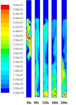
78 62 (a) Ug=9mm/s (b) Ug=12.5mm/s (c) Ug=15mm/s (d) Ug=20mm/s

79 63 (e) Ug=40mm/s Figure 2.27 Contours of the solids volume fraction under different inlet superficial velocities at 15% solids loading and ρs=930 kg/m 3 (a) Ug= 9mm/s, (b) Ug=12.5mm/s, (c) Ug=15mm/s, (d) Ug=20mm/s and (e) Ug=40mm/s Figure 2.28 shows the radial profiles of the solids holdup under different inlet superficial gas velocities at different axial locations along the column (H=0.5 m and H=1.5 m) with 15% solids loading and 930 kg/m 3 particle density. At H=0.5 m, the maximum concentration of the solid phase occurs when the inlet superficial gas velocity is the highest (Ug=40 mm/s) because more particles settle down and accumulate at the lower section of the column. At H=1.5 m, the solids volume fraction at Ug=40 mm/s is the smallest, which fluctuates around The solids volume fraction difference at H=1.5 m and H= 0.5 m is highest at Ug=40 mm/s, so particles under Ug=15 mm/s and Ug=20 mm/s can be better mixed with the liquid phase. The radial non-uniform distribution of the solid phase, which is dense at the center and dilute at the wall, can be found at both axial locations under all inlet superficial velocities. Ug=40 mm/s gives the most non-uniformity in the radial profiles of the solids holdup. Therefore, increasing the inlet superficial gas velocity will lead to a more radial non-uniform distribution of the solids holdup.

80 Solids holdup Solids holdup mm/s 20mm/s 40mm/s 15% solids loading, 930 kg/m 3 particle density (a) H=1.5 m Radial position x (m) mm/s 20mm/s 40mm/s 15% solids loading, 930 kg/m 3 particle density (b) H=0.5 m Radial position x (m) Figure 2.28 Radial profiles of the solids volume fraction under different inlet superficial gas velocities (a) H=1.5m and (b) H=0.5m

81 Average gas holdup 65 The studies on the hydrodynamics at the fully developed stage under different particle densities, which are 904 kg/m 3, 930kg/m 3 and 950kg/m 3, were conducted at Ug=15 mm/s and 15% solids loading. The average gas holdups under different particle densities are shown in Figure It can be seen that the average gas holdup under different particle densities are almost identical because the gas holdup mainly depends on the inlet superficial gas velocity % solids loading, U g =15mm/s Figure 2.29 Average gas holdup under different particle densities at Ug=15mm/s, and 15% solids loading Figure 2.30 shows the contours of the solid phase volume fraction from t=30s to 250s under different particle densities. It is noted that particles with a mean density of 904 kg/m 3 are only partially fluidized under Ug=15 mm/s, and most particles still remain packed as shown in Figure 2.30 (a). The particles with a mean density of 930 kg/m 3 are uniformly distributed along the column shown in the Figure 2.30 (b). The contours of the volume fraction of particles with a mean density of 950 kg/m 3 (Figure 2.30 (c)) indicate that the concentration of the solid phase is dense at the lower section and dilute at the upper part of the column. Thus, the particles with a higher density are easier to be fluidized in an inverse TPFB under the batch mode.

82 66 (a) 904 kg/m 3 (b) 930 kg/m 3 (c) 950 kg/m 3 Figure 2.30 Contours of the solids volume fraction with different particle densities at 15% solids loading and Ug=15mm/s (a) 904 kg/m 3, (b) 903 kg/m 3 and (c) 950kg/m 3

83 67 The time-averaged radial profiles of the solids holdup for different particle densities at two axial locations are shown in Figure At H=0.5 m, the particles with 950 kg/m 3 density have the maximum solids volume fraction. The particles with 904 kg/m 3 density have the minimum solids volume fraction at both H=0.5 m and H=1.5 m because most particles are still packed at the upper part of the column. Three types of particles with different densities all have the radial non-uniform profiles of the solids holdup. The solids holdup for particles with 904 kg/m 3 at H=1.5 m is dense at the near wall region and dilute at the center region, which is different from other particles. This is due to the liquid recirculation caused by the upward flow of gas bubbles, which fluidizes the particles at the near wall region first, so more particles at the near wall region move to the lower section of the column first.

84 Solids hodup Solids holdup kg/m3 930kg/m3 950kg/m3 (a) H=1.5 m Radial position x (m) kg/m3 930kg/m3 950kg/m3 (b) H=0.5 m Radial position x (m) Figure 2.31 Radial profiles of solids holdup with different particle densities at 15% solids loading and Ug=15mm/s (a) H=1.5m and (b) H=0.5m

85 Recirculation In an inverse TPFB under the batch liquid mode (Ul=0), the gas phase is injected into the system from the bottom of the column as bubbles, and gas bubbles flow upward. The rising gas bubbles from the bottom of the column can induce the turbulence with small eddies in the system. However, under the batch liquid mode of the inverse TPFB, the liquid is not circulated out of the column. Therefore, the recirculation of the liquid and solid phases can be observed in the inverse TPFB. The recirculation of the liquid and solid phases is an important phenomenon because it can influence the heat and mass transfer in the inverse TPFB under the batch mode. The vortex and particle recirculation are also observed in the experimental study by Sun (2017). Therefore, the investigation of the recirculation of particles is carried out in this section. The simulation is conducted under 15% solids loading and particles with 930 kg/m 3 density, but different inlet superficial velocities are employed. Figure 2.32 is the time-averaged radial profiles of the solids axial velocity at the fully developed stage. The radial non-uniform distribution of the solids axial velocity can be seen under all inlet superficial gas velocities. When Ug=15 mm/s, particles flow downward at the near wall region and the core region of the column, but upward particle flows can be found at the region between the wall and center of the column at both H=1.5 m and H=0.5 m. Particles flow upward at the core region and flow downward at the near wall region when Ug=20 mm/s at both axial locations, and particles under Ug=40 mm/s also move in both upward and downward directions. Therefore, the recirculation of particles can be found under all inlet superficial gas velocities through the radial profiles of the solids axial velocity. Besides, it can be seen that the radial profile of the solids axial velocity is most non-uniform at Ug=40 mm/s. Thus, with the increase in the inlet superficial gas velocity, the radial non-uniformity of the solids axial velocity will increase. The maximum upward and downward solids axial velocities for Ug=40 mm/s are higher than those for Ug=15 mm/s and Ug=20 mm/s, which indicates a stronger recirculation for Ug=40 mm/s than other two cases, because with the increase in the inlet superficial gas velocity, the liquid and solid phases can obtain more momentum from the gas phase.

86 Solids axial velocity (m/s) Solids axial velocity (m/s) mm/s 20mm/s 40mm/s 15% solids loading, ρ s =930 kg/m (a) H=1.5 m -0.4 Radial position x (m) mm/s 20mm/s 40mm/s 15% solids loading, ρ s =930 kg/m Radial position x (m) (b) H=0.5 m Figure 2.32 Radial profiles of the solids axial velocity under different inlet superficial gas velocities (a) H=1.5m and (b) H=0.5m

87 71 To further investigate the recirculation in the inverse TPFB under the batch mode, the flow details in all three stages of the fluidization process are studied at Ug=15 mm/s, 15% solids loading and ρ s=930 kg/m 3. Figure 2.33(a) shows the solids volume fraction contour and solids veolcity vector at the initial fluidization stage. A recirculation of particles can be observed at the bottom part of the packed bed from the velocity vector plot, where the particles descends at the near wall region on the left hand side and rise at the near wall region on the right hand side of the column, which is similar to the radial profiles of solids axial velocity shown in Figure It can be seen from Figure 2.33 (a), at the bottom part of the packed bed, particle velocities at the near wall regions are higher than the velocities at the center region of the column, which indicates that the particles at the near wall region are fluidized first at the initial fluidization stage. The solid velocity vector and solids volume fraction at the developing stage are shown in Figure 2.33 (b). A large circulation of particles can be seen at the middle and upper part of the reactor. In addition, more vortexes are found at the lower section of the column, close to the gas distributor. So the flow of particles is more disordered and the solids volume fraction distribution is very nonuniform. Figure 2.33 (c) shows the solids velocity vector and solids volume fraction at the fully developed stage. The large recirculation of particles can be found inside the column. Therefore, it can be concluded that the recirculation of particles exists at all three stages.

88 72 Middle part Bottom part (a) (b)

89 73 Solids volume fraction (c) Solids velocity vector Figure 2.33 Instantaneous volume fraction contour (left) and particle velocity vector contour (right) (a) Initial fluidization stage, (b) Developing stage and (c) Fully developed stage 2.6 Conclusions A three-phase Eulerian-Eulerian CFD model coupled with the kinetic theory of the granular flow has been developed for simulation of the inverse TPFB under the batch liquid mode, and it is validated with experimental data. A two-dimensional numerical simulation has been conducted in order to study the hydrodynamics and flow structures in an inverse TPFB. The flow development in the inverse three-phase fluidization process is investigated under conditions of Ug=15 mm/s, 15% solids loading, and 903 kg/m 3 particle density. The CFD results show that flow development in the inverse three-phase fluidization system can be divided into three stages, which are the initial fluidization stage, developing stage and fully developed stage based on the axial profile of the solid phase. The fluidization of particles was found to begin from the near wall region firstly due to the liquid recirculation

90 74 caused by the upward gas flow at the initial fluidization stage. The radial non-uniform profile of the gas holdup, solids holdup and solids axial velocity are shown at all three stages. The radial non-uniformity decreases with time, so the radial flow structure is more uniform at the fully developed stage. In addition, it is noted that a higher solids volume fraction occurs where particles flow upward, and a lower solids volume fraction is at where the particle moves downward at all three stages. The effect of the solids loading on the flow structure has been studied through CFD modeling under Ug=15 mm/s. It is noted that the time to reach to the developing stage and fully developed stage is longer with a higher solids loading, so the particles with higher solids loading are more difficult to be fluidized. Besides, by applying different inlet superficial velocities with 15% solids loading, it is noted the time to reach to the developing stage and fully developed stage is reduced with the increase in the inlet superficial gas velocity under the same solids loading. The radial non-uniformity of the solids holdup increases with the increase in the solids loading. However, the solids loading has almost no effect on the radial distribution of the gas holdup. The general flow structure at the fully developed stage including the radial solids distribution, axial solids distribution and gas holdup are also investigated under different inlet superficial gas velocities and particle densities. More particles move downward when increasing Ug. Particles are easier to be fluidized when its density is close to the liquid phase density, so the solid phase becomes denser at the lower section and dilute at the upper section of column when increasing the particle density. For the radial flow structure, the radial non-uniform profile of the solids holdup is observed at different inlet superficial velocities and particle densities. The radial non-uniformity of the solids holdup increases when increasing Ug, but it is not affected by the particle density. The particle density has almost no effect on the average holdup as well. In addition, it is found that the recirculation of particles exists at all three stages in the inverse fluidized bed under the batch liquid mode.

91 75 Reference Ansys. Inc. (2014). Fluent 16.0 User s Guide. Bandaru, K. S. V. S. R., Murthy, D. V. S., & Krishnaiah, K. (2007). Some hydrodynamic aspects of 3-phase inverse fluidized bed. China Particuology, 5(5), Buffière, P., & Moletta, R. (1999). Some hydrodynamic characteristics of inverse three phase fluidized-bed reactors. Chemical Engineering Science, 54(9), Cho, Y. J., Park, H. Y., Kim, S. W., Kang, Y., & Kim, S. D. (2002). Heat transfer and hydrodynamics in two- and three-phase inverse fluidized beds. Industrial and Engineering Chemistry Research, 41(8), Comte, M. P., Bastoul, D., Hebrard, G., Roustan, M., & Lazarova, V. (1997). Hydrodynamics of a three-phase fluidized bed - The inverse turbulent bed. Chemical Engineering Science, 52(21 22), Ding, J., & Gidaspow, D. (1990). A bubbling fluidization model using kinetic theory of granular flow. AIChE Journal, 36(4), Fan, L. S., Muroyama, K., & Chern, S. H. (1982). Hydrodynamic characteristics of inverse fluidization in liquid-solid and gas-liquid-solid systems. The Chemical Engineering Journal, 24(2), Feng, W., Wen, J., Fan, J., Yuan, Q., Jia, X., & Sun, Y. (2005). Local hydrodynamics of gas liquid-nanoparticles three-phase fluidization. Chemical Engineering Science, 60(24), Gidaspow, D. (1994). Multiphase Flow and Fluidization: Continuu and Kinetic Theory Descriptions. Boston: Acad. Press. Grevskott, S., Sannaes, B. H., Dudukovic, M. P., Hjarbo, K. W., & Svendsen, H. F. (1996). Liquid circulation, bubble size distributions, and solid movement in two- and threephase bubble columns. Chemical Engineering Science, 51(10), Hamidipour, M., Chen, J., & Larachi, F. (2012). CFD study on hydrodynamics in threephase fluidized beds Application of turbulence models and experimental validation. Chemical Engineering Science, 78, Hillmer, G., & Weismantel, L. (1994). Investigations and Modelling Columns of Slurry

92 76 Bubble. Science, 49(6), Ibrahim, Y. A. A., Briens, C. L., Margaritis, A., & Bergongnou, M. A. (1996). Hydrodynamic Characteristics of a Three-Phase Inverse Fluidized-Bed Column. AIChE Journal, 42(7), Lee, D. H., Epstein, N., & Grace, J. R. (2000). Hydrodynamic Transition from Fixed to Fully Fluidized Beds for Three-Phase Inverse Fluidization. Korean Journal of Chemical Engineering, 17(6), Li, W., & Zhong, W. (2015). CFD simulation of hydrodynamics of gas-liquid-solid threephase bubble column. Powder Technology, 286, Li, Y., Zhang, J., & Fan, L.-S. (1999). Numerical simulation of gas liquid solid fluidization systems using a combined CFD-VOF-DPM method: bubble wake behavior. Chemical Engineering Science, 54(21), Lun, C. K. K., Savage, S. B., Jeffrey, D. J., & Chepurniy, N. (1984). Kinetic theories for granular flow: Inelastic particles in Couette flow and slightly inelastic particles in a general flowfield. Journal of Fluid Mechanics, 140(1), Muroyama, K., & Fan, L. S. (1985). Fundamentals of gas liquid solid fluidization. AIChE Journal, 31(1), Panneerselvam, R., Savithri, S., & Surender, G. D. (2009). CFD simulation of hydrodynamics of gas liquid solid fluidised bed reactor. Chemical Engineering Science, 64(6), Renganathan, T., & Krishnaiah, K. (2008). Prediction of Minimum Fluidization Velocity in Two and Three Phase Inverse Fluidized Beds. The Canadian Journal of Chemical Engineering, 81(3 4), Schaeffer, D. G. (1987). Instability in the evolution equations describing incompressible granular flow. Journal of Differential Equations, 66(1), Schiller, L., & Naumann, A. (1935). A drag coefficient correlation. Z. Ver. Deutsch. Ing, 77, Sun, X. (2017). Bubble induced Inverse Gas-liquid-solid Fluidized bed. University of Western Ontario. Syamlal, M., Rogers, W., & O`Brien, T. J. (1993). MFIX documentation theory guide.

93 77 United States. Wen, J., & Xu, S. (1998). Local hydrodynamics in a gas-liquid-solid three-phase bubble column reactor. Chemical Engineering Journal, 70(1), Wu, Y., & Gidaspow, D. (2000). Hydrodynamic simulation of methanol synthesis in gasliquid slurry bubble column reactors. Chemical Engineering Science, 55(3), Yakhot, V., & Orszag, S. A. (1986). Renormalization group analysis of turbulence. I. Basic theory. Journal of Scientific Computing, 1(1), Zhang, D. Z., & Vanderheyden, W. B. (2002). The effects of mesoscale structures on the disperse two-phase flows and their closures for dilute suspensions. Int. J. Multiphase Flows, 28(5),

94 78 Chapter 3 3 Modification of the CFD Model Based on the Bubble Size Adjustment for the Inverse Three-phase Fluidized Bed 3.1 Introduction Fluidization is a process that converts particles from the solid like state to a fluid like state by injecting liquid or gas flow into the system. With different fluidizing agents, fluidized beds can be categorized as the liquid-solid two-phase fluidization, gas-solid two-phase fluidization and gas-liquid-solid three-phase fluidization. The gas-liquid-solid three-phase fluidized bed (TPFB) has many applications in chemical, biochemical, petrochemical industries because it has a higher contact efficiency among each phase and good mass and heat transfer features (Muroyama & Fan, 1985). Fluidized beds can be further divided into the upward fluidized bed and inverse fluidized bed based on the flow direction of the fluidizing agent. In inverse TPFBs, the particle density is usually less than the liquid density, so the fluidization process will start when the drag force and gravity on the particle are balanced with the buoyancy force. The inverse gas-liquid-solid (GLS) fluidized bed can be operated under a continuous mode or batch liquid mode. Only gas is introduced into the fluidized bed at a certain velocity to fluidize the liquid and solids inside the column under the batch liquid mode. Under the continuous mode, both gas and liquid work as the fluidizing agents to fluidize the packed solids inside the fluidized bed. Compared with the traditional upward three-phase fluidized bed, the inverse TPFB has some advantages such as the lower energy cost. In an inverse TPFB, the fluidization process will go through the fixed bed with dispersed bubble regime, bubbling fluidized bed regime, transition regime and slugging fluidized bed regime when increasing the liquid or gas velocity (Fan et al., 1982). Three significant superficial gas velocities have been defined to distinguish the flow regimes in an inverse TPFB under the batch liquid mode, which are (1) the minimum gas fluidization velocity Ug1 that can break the fixed bed, (2) velocity Ug2 is the velocity that can let some particle to reach the bottom of the column, and (3) velocity Ug3 that can result in a uniform axial

95 79 particle distribution (Comte et al., 1997; Sun, 2017). It was found that Ug2 and Ug3 will decrease with an increase in the solids loading or particle density. Other parameters and characteristics of the hydrodynamics in the inverse TPFB have been studied by a few researchers. The minimum liquid fluidization velocity was found to decrease with the increase in the gas velocity, and the average liquid holdup and gas holdup was found to increase with the increase in the superficial gas and liquid velocities (Bandaru et al., 2007; Cho et al., 2002; D. H. Lee et al., 2000). A correlation was developed by Renganathan & Krishnaiah (2008), which can predict the minimum fluidization velocity in the inverse TPFB under both the batch mode and continuous mode. Ibrahim et al. (1996) and Bandaru et al. (2007) studied the axial phase holdup in the inverse TPFB. The solid phase was found to become dilute at the top of the column and dense at the bottom when increasing the gas velocity or liquid velocity. Later, Sun (2017) reported similar results on the average holdup and axial distribution of each phases in the inverse TPFB under the batch mode. However, no studies on the hydrodynamics and flow patterns of an inverse TPFB in the radial direction were reported in the literatures. For the bubble induced three-phase fluidization, the gas, which is introduced into the column, is usually present in the form of small bubbles with the help of the gas distributor. It was found that small gas bubbles and the density difference between the solid phase and the liquid-gas mixture would result in the liquid recirculation, which causes the bed to expand in the inverse TPFB under the batch liquid mode. (Buffière & Moletta, 1999; Renganathan & Krishnaiah, 2008). In that case, the bubble behavior has become an important role in the design and operation of the inverse TPFB under the batch liquid mode since bubbles related to the mass transfer and mixing in the TPFB. However, only a fewer literatures reported the relationship between the average bubble size, the inlet superficial gas velocity and the gas holdup, such as a correlation for an upward gas-liquid bubble column under the superficial gas velocities ranging from 0-12 cm/s (Jamialahmadi & Muller-Steinhagen, 1993). Less research works on the bubble behavior in the inverse TPFB were carried during the past decades.

96 80 For the inverse gas-liquid two-phase bubble column, Son et al. (2004) studied the bubble behavior and properties in a gas-liquid countercurrent flow bubble column, which is used for wastewater treatment. Four pipes in 6.35 mm diameter with 28 holes were used as the gas distributor in this experimental study, and the gas distributor is evenly installed at the bottom of the column. A correlation to calculate the bubble size based on the superficial liquid velocity and gas velocity was developed in their study. It was also found that the gas holdup under the batch liquid mode is smaller than the gas holdup under the continuous mode in a gas-liquid countercurrent bubble column. Compared to the gas-liquid two-phase flow in a bubble column, less researchers reported studies on the bubble behaviors in inverse three-phase fluidized beds. Cho et al. (2002) reported that the bubble size and bubble rising velocity will increase when increasing the gas velocity in an inverse TPFB under the continuous mode. Later, Son et al. (2007) used the same experimental equipment that was used by Son et al. (2004) to study the bubble behaviors in an inverse TPFB under the continuous mode. The experimental study was conducted at Ul=10 mm/s - 50 mm/s, Ug= 0.5 mm/s - 8 mm/s and ρ s =877.3 kg/m kg/m 3. A correlation for the bubble size and bubble rising velocity based on the drift flux model was developed. It was also found that the bubble size increases with the increase in the gas velocity, liquid viscosity or liquid velocity, but it will decrease when increasing the particle density. The bubble rising velocity was found to increase with an increase in the gas velocity or liquid viscosity. However, no studies have reported the average bubble size in the inverse TPFB under the batch liquid mode (Ul=0) due to the inadequate experiments and the limitation of the visualization techniques. The CFD method allows the model to include the effect of the bubble size, which can be used to further study the relationship between the bubble size and the inlet superficial gas velocity. Thus, the modification of the CFD model proposed in the previous work for the simulation of the flow in the inverse TPFB is carried out to include the effect of the bubble size on the flow field in the inverse TPFB. The Eulerian-Lagrangian approach and Eulerian-Eulerian approach are the two main methods that, are used to simulate the three-phase flows in fluidized beds. In the Eulerian-

97 81 Lagrangian approach, the liquid and gas phases are treated as the continuous phases. The solid phase is treated as the discrete phase, and each individual particle is tracked by solving the Lagrangian force balance equation. Due to the high computational cost, the Eulerian- Lagrangian approach is used when the volume fraction of discrete phase is low. Thus, the Eulerian-Eulerian approach coupled with the kinetic theory of the granular flow (KTGP) is widely used for simulating the flow in the TPFBs. Each phase is treated as a continuum solved by governing equations in the Eulerian-Eulerian approach. The KTGP is used to calculate the solid phase pressure, viscosity and stress. The Eulerian-Eulerian approach can be divided into the pseudo two-fluid model and three-fluid Eulerian-Eulerian model when simulating three-phase flows. The pseudo two-fluid model is used when the particle or bubble size is small, the volume fraction of the solid or gas phase is low and the slip velocity between the two phases is low. Therefore, the liquid-gas or liquid-solid can be treated as one phase. Thus, the three-phase flows in the fluidized bed can be simplified to a two-phase flows. The pseudo two-fluid model is often used to simulate the flow in the three-phase slurry fluidized bed or the fluidized bed that uses nanoparticles (Feng et al., 2005; Grevskott et al., 1996; Hillmer & Weismantel, 1994; Wen & Xu, 1998). Besides, the Eulerian-Eulerian three-fluid model is often needed to simulate the flow in the gas-liquidsolid TPFB. Due to the complicated interacton among each phase in the TPFB, fewer CFD studies have been carried out to predict the hydrodynamcis and flow patterns in the TPFB based on the three-fluid Eulerian-Eulerian model. Panneerselvam et al. (2009) studied the hydrodynamics and flow pattern in an upward TPFB numerically. Two different superficial gas velocities, Ug = 0.2 m/s and Ug=0.4 m/s, were used in the simulation. The mean bubble sizes used for the gas phase at each inlet superficial gas velocity are 13 mm and 2 mm, respectively, which was determined by comparing the gas holdup from the simulation results with that from the experimental data. Hamidipour et al. (2012) conducted the same numerical study as Panneerselvam et al. (2009) by using the three-fluid Eulerian-Eulerian model with the KTGP. The same bubble size was used in their study as well. Li and Zhong (2015) carried out a numerical study in a TPFB based on the three-fluid Eulerian-Eulerian model. The performances of different drag models between each phase were compared. The range of the inlet superfical gas velocity in the study was from m/s to 0.33 m/s,

98 82 but only one mean bubble size of m was used in the simulations for different inlet superfical gas veolcities. It is believed that the bubble size in a TPFB increases with the increase in the superficial gas velocity. (Kulkarni & Joshi, 2005; Son et al., 2004, 2007). However, most numerical stuides on TPFBs used only one bubble size for the gas phase even under the different inlet superfical gas velocities. Thus, the objective of this study is to modify the CFD model for the simulation of the inverse TPFB under the batch liquid mode proposed in the previous study by adjusting the bubble size under different superfical gas velocities. Also, since the numerical studies on the bubble behavior in the inverse TPFB were conducted only for a very small operating range, investigations on the flows in an inverse TPFB under wide range of different operating conditions be conducted. And a correaltion to predict the bubble size under different inlet superfical gas velocities will be developed as well. 3.2 Experimental setup of the inverse three-phase fluidized bed The proposed CFD model has been validated based on the experimental data by Sun (2017). The configuration of the inverse TPFB used by Sun (2017) is shown in Figure 3.1. The column is made of PVC with m in diameter and 3 m in height. The ring shape porous quartz gas distributor with an 8.7 cm outer diameter and a 2.7 cm inner diameter, which can generate very small bubbles, is placed at the bottom of the column. The tap water, air and particles (ρs=930 kg/m 3 ) are used as liquid, gas and solid phases in the experiment. The tap water and particles are injected into the column before the experiment starts, resulting in the floated particles at the top surface of the water because the particle density is lower than the density of water. During the experiment, only the gas is continuously introduced into the column through the gas distributor, and there is no outflow for particles and liquid. The gas phase is injected into the column as small bubbles from the bottom of the column through the gas distributor, and bubbles leaves the column through the top of the column. The superficial gas velocity at the inlet is from 0 mm/s to 60 mm/s. With an increase in the inlet superficial gas velocity, the coalescence of small bubbles can be observed. The experiment is carried out under ambient temperature and pressure.

99 83 In this study, the hydrodynamics in the inverse TPFB will be simulated under different inlet superficial gas velocities with its corresponding bubble size. Therefore, different bubble sizes will be used under different inlet superficial gas velocities. The summary of the operating conditions and properties of each phase are shown in Table Column 2 Bubble 3 Liquid 4 Solid particles 5 Rotameters 6 Pressure gauge 7 Gas distributor 8 Liquid inlet/outlet valve 9 Manometer Figure 3.1 Configuration of the experimental setup of the inverse three-phase fluidized bed (Sun, 2017)