ρ x + fv f 'w + F x ρ y fu + F y Fundamental Equation in z coordinate p = ρrt or pα = RT Du uv tanφ Dv Dt + u2 tanφ + vw a a = 1 p Dw Dt u2 + v 2

Transcription

1 Fundamental Equation in z coordinate p = ρrt or pα = RT Du uv tanφ + uw Dt a a = 1 p ρ x + fv f 'w + F x Dv Dt + u2 tanφ + vw a a = 1 p ρ y fu + F y Dw Dt u2 + v 2 = 1 p a ρ z g + f 'u + F z Dρ Dt + ρ U = 0 DT c p Dt α Dp Dt = L(C E) + Q rad + Q diff (for full moist model, equation of water vapor is also included) f --- 2Ωsinφ f ' --- 2Ωcosφ C condensation E evaporation 6 equations 6 unknowns: u, v, w, p, ρ, T 4 dimensions x, y, z, t SCALE ANALYSIS Equations above describe motions of the atmosphere at all scales from mm to 1000s km. If we are interested in the motions that matter to our day-to-day weather (i.e., phenomenology described by synoptic weather map), we may want to eliminate or filter out the unwanted type of motions, such as sound waves. Elimination of terms on scaling considerations not only has the advantage of simplifying the mathematics, but also elimination of the unwanted motions which may corrupt the numerical solution for the wanted motion (e.g., the first attempt of Richardson on numerical weather forecast failed because of the equations he used contain the acoustic and gravity waves). To determine the dominant balance of terms in the equations, and apply approximations to simplify their solutions, we define the following characteristics scales of the field variables based on observed values from midlatitude synoptic systems. These estimates of scales are then substituted into the equations to determine which terms are of the same (larger) order of magnitude---the balance of leading orders. Note that scale analysis in general only tells what but not why. 1

2 U 10m s 1 W 10 2 m s 1 L 10 6 m H 10 4 m δp/ρ 10 3 m 2 s 2 T L /U 10 5 s horizontal velocity vertical velocity horizoantl length depth scale (vertial length) horizonal pressure fluctuation scale advective time scale f 10 4 s 1 planetary vorticity, time scale of earth rotation, Coriolis acceleration on relative motion Table 2.1 shows the characteristic magnitude of each term in the equation set above. 1. Geostrophic approximation It is apparent from Table 2.1 that for midlatitude synoptic scale disturbances the Coriolis force and the pressure gradient force are in approximate balance. Retaining only these two terms in the equations gives as a first approximation the geostrophic relationship fv 1 p ρ x ; fu 1 p (2.22) ρ y which is just a diagnostic relationship. To predict time evolution, we need keep the higher order term---the time tendency term and inertial terms. For example, 2

3 Du Dt u t + u u x + v u y U 2 / L 10 4 For the geostrophic relationship to hold, R o U f 0 L 1. + w u z 1 p ρ x + fv By analogy to the geostrophic approximation, it is possible to define horizontal geostrophic wind V g = iu g + jv g, which satisfies (2.22) identically. In vectorial form, V g k 1 p (2.23) ρ f It should be kept in mind that (2.23) always defines the geostrophic wind, but only for large-scale motions away from equator should (2.22) apply as an approximation to the actual horizontal wind field. The typical accuracy of (2.22) is within 10-15% of the actual wind. Homework: show p V g or p V g = 0 f 0 U Hydrostatic approximation Similar scale analysis leads to, to a high degree of accuracy, the hydrostatic equilibrium, that is, the pressure at any point is simply equal the weight of the of a unit cross-section column of air above that point. However, the above analysis is somehow misleading. It is not sufficient to show merely that the vertical acceleration is small compared to g. Because only that part of pressure field that varies horizontally is directly coupled to the horizontal velocity field, it is actually necessary to show that the horizontally varying pressure component is itself in hydrostatic equilibrium with the horizontally varying density field. To do this it is conventional to first define a standard pressure p 0 (z), which is the horizontally averaged pressure at each height, and a corresponding standard density ρ 0 (z), defined as such so that p 0 (z) and ρ 0 (z) are in exact hydrostatic balance: 3

4 Therefore, for synoptic motion, vertical accelerations are negligible and the vertical velocity cannot be determined from the vertical momentum equation. Can be transformed to p-coordinate, because p is a monotonic and single-valued function of z. 3. Scale analysis of the Continuity Equation 1 Dρ ρ Dt + U = 0 (2.31) Following the technique developed above, and assuming that ρ'/ ρ 0 approximate the continuity equation (2.31) as 1, we 4

5 1 ρ' + U ρ' ρ t + w dρ 0 + U ρ 0 dz 0 A ρ' U ρ 0 L A. For synoptic scale motion: ρ'/ ρ 0 ~ 10 2 B W H C 10 1 U L 10 7 s s s 1 B. For motion in which the depth scale H is comparable to the density scale height, d ln ρ 0 / dz H 1 10km. C. U = u x + v y + w, for synoptic motions the first two terms tend to cancel each z other, giving rise to a sum that is an order smaller. Thus, terms B and C are each an order of magnitude larger than term A, and to a first approximation, terms B and C balance each other in the continuity equation. u x + v y + w z + w d dz (ln ρ ) = 0 0 or in vectorial form (ρ 0 U) = 0 (2.34) This means that for synoptic scale motions the mass flux computed using the basic state density is nondivergent. For purely horizontal flow, the atmosphere behaves as though it were an incompressible fluid. This is similar to, but not the same as the idealization of incompressibility used in fluid mechanics. However, an incompressible fluid has density constant following the motion: Dρ Dt = 0 Thus, by (2.31), velocity divergence vanishes ( U = 0, used in Boussinesq sets of equations 1 ) in an incompressible fluid, which is not the same as (2.34). 1 The Boussinesq approximation ignores all variations of density of a fluid in the momentum equations, except when associated with the gravitational (or buoyancy) term. Boussinesq sets of equations use U = 0, but this should absolutely not allow one to go back and use (2.31) to say that Dρ = 0 ; the evolution of density is given by the Dt thermodynamic equation in conjunction with an equation of state. However, using p-coordinates, the Boussinesq equations for atmospheric circulation do not need these approximation in continuity equations. Let the oceanographers to worry about this issue. 5

6 It is also worthy of note that equation (2.34) is where the eponymous anelastic approximation arises: the elastic compressibility of the fluid is neglected (by assuming T ~ U / L, in which time scale the sound waves do not dominate --- A term drops out of the equation), and this serves to eliminate sound waves. This approximation is also referred to as weak Boussinesq approximation. Because if we let ρ 0 (z) be a constant, the anelastic equations become identical to the Boussinesq equations. 6

7 GOVERNING EQUATION OF MOTION IN PRESSURE COORDINATES 1. Horizontal momentum equations Recall equation (1.25) and (1.26), 1 p = Φ ρ x z x p 1 p = Φ ρ y z y p In vectorial form, let the horizontal velocity V = iu + jv, the horizontal momentum equation in isobaric coordinate can be written as DV Dt + fk V = Φ (3.2) p where p is the horizontal gradient operator applied with pressure held constant. (some nuances about the observation of the horizontal wind on isobaric surface) In p-coor, variables are function of x, y, p,t, and total derivative D Dt = t + u x + v y + ω p where ω Dp is the pressure change following the motion, which plays the same role in Dt p-coor as w does in z-coor. 2. Continuity equation It is possible to transform the continuity equation (2.31) from z-coor to p-coor. But I leave it to you. However, it is simpler to directly derive the isobaric form by considering a Lagrangian control volume δv = δ xδ yδz and applying the hydrostatic equation δ p = ρgδz to express the volume element as δv = δ xδ yδ p / (ρg). The mass of this fluid element, which is conserved following the motion, is then δ M = ρδv = δ xδ yδz / g, thus 1 δ M D Dt (δ M ) = g δ xδ yδ p D Dt δ xδ yδ p g = 0 chain rule and change order of the differential operators 1 δ x δ or Dx Dt + 1 δ y δ δu δ x + δv δ y + δω δ p = 0 Dy Dt + 1 δ p δ Dp Dt = 0 7

8 Taking the limit δ x,δ y,δ p 0 and observing that δ x and δ y are evaluated at constant pressure, we derive the continuity equation in the isobaric system: u x + v y + ω p = 0 This form of the continuity equation contains no reference to the density field and does not involve time derivatives---the chief advantages of the isobaric coordinates. 3. Thermodynamic Energy Equation From (2.42) DT c p Dt α Dp Dt = J, we have the following written in isobaric system: T c p t + u T x + v T y + ω T p αω = J This may be further, by combining the last two terms of the lhs, written as T t + u T x + v T y S pω = J c p where p S p RT c p p T p = T θ θ p (3.7, derive this) is the static stability parameter for the isobaric system. Using (2.49) and the hydrostatic equation, (3.7) may be rewritten as S p = (Γ d Γ) / ρg Thus, S p is positive provided that the lapse rate is less than dry adiabatic. Scale analysis of ω Dp Dt = p p + V p + w t z shows that it is quite a good approximation to let ω = ρgw Put together, we now have 8

9 p = ρrt or pα = RT u t + u u x + v u y + ω u p v t + u v x + v v y + ω v Φ p = α u x + v y + ω p = 0 Fundamental Equation in p-coordinate uv tanφ = + uω f 'ω + fv + a ρga ρg Φ x + F rx p = u2 tanφ a + vω ρga fu Φ y + F ry c p OR T t + u T x + v T y αω = L(C E) + Q rad + Q diff T t + u T x + v T y = Sω + L c p (C E) + q rad + q diff where q rad = Q rad / c p q diff = Q diff / c p S = T θ (static stability) θ p r t + u r x + v r y + ω r = Sources Sinks p after the scale ananlysis of the first round 9

10 p = ρrt or pα = RT u t + u u x + v u y + ω u Φ = fv p x + F rx v t + u v x + v v y + ω v Φ = fu p y + F ry Φ p = α = RT p u x + v y + ω p = 0 c p OR T t + u T x + v T y αω = L(C E) + Q rad + Q diff T t + u T x + v T y = Sω + L c p (C E) + q rad + q diff where q rad = Q rad / c p q diff = Q diff / c p S = T θ (static stability) θ p (see page 147, equations (6.1-4)) 10

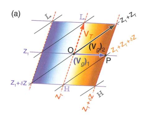
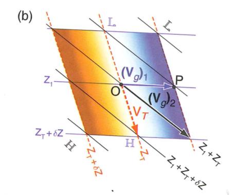
11 Geostrophic wind Thermal Wind fv g = k p Φ fv g = Φ x fu g = Φ y p v g = 1 f x Φ p p u g = 1 f y using hydrostatic equation: Φ p = α = RT p, then, p v g p = v g ln p = R f p u g p = u g ln p = R f or in vectorial form V g ln p = R f k pt thermal wind (3.30) Designating the thermal wind vector by V T, we may integrate (3.30) from pressure level p 0 to p 1 (p 1 < p 0 ) to get V T V g (p 1 ) V g (p 0 ) = R k p T f d ln p (3.31) p 0 Letting T denote the mean temperature in the layer between pressure level p 0 and p 1, than the thermal wind relation can be written as: V T = R f k T ln p 0 p 1 = 1 f k (Φ Φ ) = g 1 0 f k Z T (3.35) The equivalence of these equations can be verified readily by integrating the hydrostatic equation vertically from p 0 to p 1. Φ p p 1 T x T y p p ( ) With (3.35), it is therefore possible to obtain a reasonable estimate of the horizontal temperature advection and its vertical dependence at a given location solely from data on the vertical profile of the wind of a single sounding. In the meantime, the geostrophic wind at any level can be estimated from the mean temperature field, provided that the geostrophic velocity is known at a single level. Counterclockwise turning with height cold advection Clockwise turning (veering) with height warm advection 11

12 12

13 13

14 Homework A: read page 73 carefully and derive the hypsometric equation Φ 1 Φ 0 gz T = R T ln p 0 (3.34) Homework B: Use the knowledge of page 73 and the hypsometric equation above to estimate the expected tilt of 500 hpa pressure surface between the tropics and the pole based on the following conditions and assumptions: (i) T only varies only merdionally, i.e., isothermal in vertical; (ii) surface pressure p s = 1000 hpa; (iii) equator-to-pole temperature difference ΔT equator pole = 40K. And draw picture to demonstrate the results schematically. p 1 Hints: use equation Δz equator pole = RΔT equator pole g ln p s p 500 and diagram below as clues. 14

15 Barotropic flow Barotropic defined by ρ = ρ(p), so the isobaric surface is also the surface of constant density. For an ideal gas, the isobaric surface will be also isothermal for the barotropic atmosphere. Thus p T = 0 in a barotropic ideal-gas atmosphere and V g ln p = R f k pt = 0 and geostrophic wind is independent of p (vertical coordinate). Barotropy produces a very strong constraint on the motions and forms basis of much of theoretical understanding. If ρ = ρ( p,t ), then the flow is baroclinic. 15