Regional Curves of Hydraulic Geometry for Wadeable Streams. Marin and Sonoma Counties, San Francisco Bay Area. Data Summary Report.

Transcription

1 Regional Curves of Hydraulic Geometry for Wadeable Streams in Marin and Sonoma Counties, San Francisco Bay Area Data Summary Report May 10, 2013 Laurel Collins Watershed Sciences Berkeley, CA Roger Leventhal, P.E. Marin County Flood Control District San Rafael, CA 1

2 MARIN AND SONOMA COUNTIES REGIONAL CURVES REPORT This page intentionally left blank 2

3 This project was partially funded by an EPA grant under the Estuary 2100 project administered by the San Francisco Estuary Project. The report was prepared by: Laurel M. Collins Watershed Sciences 1128 Fresno Street Berkeley, CA Roger Leventhal, P.E. FarWest Restoration Engineering/Waterways Restoration Institute 703 West Street Petaluma, CA and currently at Marin County Flood Control District 3501 Civic Center Drive, Suite 304 San Rafael, CA Acknowledgements We wish to thank Professor Bill Dietrich of UC Berkeley for providing guidance for the initial development the field data collection sheet. We also wish to thanks Dan Mecklenberg of the State of Ohio Department of Natural Resources for not only providing his geomorphic analysis spreadsheet STREAMS as a free download to the creek community but for answering our specific questions that came up during our use of the spreadsheet. We owe our deep gratitude to the many assistants that helped with field data collection, especially Kristen Wood, Sumner Collins. We also thank Terry Henry of the US National Forest Service for providing her seasonal staff including Kyle Wright, Peter McPherson, Tyler Ward, Okira Sugita-Vasquez, and Julian Hein. We thank Jamie Kass and Kristen Cayce of the San Francisco Estuary Institute for GIS analysis of drainage area and drainage network length We are very thankful to Judy Kelly and her staff of the San Francisco Estuary Partnership (SFEP) particularly Jennifer Krebs, James Muller and Paula Trigueros for their assistance and oversight of the project. We also thank Ms. Luisa Valiela and the US Environmental Protection Agency for their support. Finally, we are indebted to Ms. Ann Riley of the California Regional Water Quality Control Board for her championing and promotion of this project. 3

4 MARIN AND SONOMA COUNTIES REGIONAL CURVES REPORT This page intentionally left blank 2

5 Contents 1.0 INTRODUCTION BACKGROUND TO BANKFULL CHANNEL DIMENSIONS BACKGROUND TO HYDRAULIC GEOMETRY AND REGIONAL CURVE ANALYSIS STUDY LIMITATIONS DATA COLLECTION METHODS SITE SELECTION METHODS FIELD DATA COLLECTION METHODS GIS DATA ANALYSIS METHODS BANKFULL DISCHARGE CALCULATION METHODS RESULTS CONCLUSIONS AND NEXT STEPS REFERENCES Tables and Figures Figure 1: Graph of flood frequency and sediment discharge showing effective and bankfull discharge. From Wolman and Miller, Figure 2: A natural river at bankfull flow Figure 3: Schematic cross-section of a river showing bankfull depth (from Rosgen 1996)... 9 Figure 4: Original Leopold Regional Curves (1978) for bankfull dimensions versus drainage area (reprinted from Rosgen 1996) Figure 5: Location of Marin County Survey Sites. San Antonio Creek straddles the Marin and Sonoma County line Figure 6: Location of Sonoma County Survey Sites Figure 7: Frequency Distribution of Field Sites by Channel Slope Class Figure 8: Frequency Distribution of Field Sites by Drainage Area Class Figure 9: Frequency Distribution of Field Sites by Dominant Geomorphic Type Figure 10: Frequency Distribution of Field Sites by Rosgen Stream Class Figure 11: Plot of Bankfull Cross-Sectional Area versus Drainage Area Figure 12: Plot of Bankfull Width versus Drainage Area Figure 13: Plot of Bankfull Depth versus Drainage Area Figure 14: Plot of Bankfull Floodprone Width versus Drainage Area Figure 15: Plot of Bankfull Floodprone Width versus Drainage Area with unstable sites of Rosgen Stream Class F and G channels removed from the analysis Figure 16: Plot of Bankfull Flow versus Drainage Area Figure 17: Plot of Mean Depth to Max Depth

6 MARIN AND SONOMA COUNTIES REGIONAL CURVES REPORT Figure 18: Plot of Manning s n by Rosgen Channel Type Figure 19: Plot of Bankfull Mean Velocity versus Drainage Area Figure 20: Plot of Drainage Network Length by Bankfull Cross Sectional Area Table 1: Calculated Recurrence Interval for Bankfull Discharge at Gage Sites..25 Table 2: List of Field Sites.. 39 Appendix A Original Leopold Expression of Hydraulic geometry Appendix B Rosgen Stream Types 4

7 1.0 INTRODUCTION This project report presents the results of a multi-year effort to develop regional design curves of hydraulic channel geometry ( regional curves ) for wadeable streams in Marin and Sonoma Counties in the San Francisco Bay Area. The project was funded in part by the US EPA under the Estuary 2100 program grant through the San Francisco Estuary Partnership (SFEP). Through this project, we have performed geomorphic field surveys at 45 sites in Marin and Sonoma Counties to develop a series of plots of hydraulic geometry dimensions of crosssectional area, width, and depth at what was identified from field surveys as the possible channel stage associated with the discharge that tends to maintain stable channel geometry. Rivers develop in a stochastic, heterogeneous world of varying local conditions and widely ranging inputs of water and sediment. Despite this they develop a persistent morphology in which channel geometry (width and mean depth) is on the average relatively stable. In alluvial valleys there is a central tendency of stable streams to form a floodplain bench. Although the term that defines the flow that maintains stable channel geometry could be associated with bankfull flow and/or effective discharge, we chose to use the term bankfull flow to represent the discharge stage and hydraulic geometry associated with the formation of a floodplain bench identified in the field. This report presents the results of the first phase of data analysis covered under this grant that satisfies (and in fact exceeds) the requirements of the original EPA grant that partially funded this study. These requirements include regional curve plots of bankfull width, depth and cross-sectional area as a function of drainage area. In addition, to these plots, we have included several other plots of various data parameters along with our initial interpretation of the results. Subsequent phases of data analysis will include a more in-depth stratification and analysis of the data to look for statistically meaningful correlations of other watershed and channel data parameters to provide greater insight of the causative influence s on stable channel geometry. This next phase of data analysis will depend upon future funding but will include statistical analyses of the influences of upstream channel network length, precipitation, geology, Rosgen Stream Class, and geomorphic setting. 1.1 Background to Bankfull Channel Dimensions The concept of stable or bankfull flow and dimension is based upon observations and measurements that natural stream channels are created and maintained by moderate, frequent flow events because these events move the most sediment over time and thus do the most work to form the creek channel dimensions (i.e. width, depth, area and planform). These flow events were defined by Dunne and Leopold (1978): The bankfull stage corresponds to the discharge at which channel maintenance is the most effective, that is, the discharge at which moving sediment, 5

8 MARIN AND SONOMA COUNTIES REGIONAL CURVES REPORT forming or removing bars, forming or changing bends and meanders, and generally doing work that results in the average morphologic characteristics of channels. As measured in the field, bankfull stage defines the boundary between the active channel and its floodplain. Over the long-term, bankfull flow carries the bulk of the systems sediment supply and forms the equilibrium channel dimensions in alluvial channels (i.e. channel free to adjust their bed and banks). The bankfull flow is commonly associated with recurrence intervals between 1.2 and 1.8 years. Lesser discharges occur more often but lack the shear forces to move enough sediment over time to define the channel morphology and higher flood flows may have greater stream power to move sediment, yet they do not occur with sufficient frequency to define and maintain channel geometry. The floodplain feature, when one is present, is a relatively flat bench or plain at the level of bankfull that carries floods, which are flows that exceed bankfull stage. Higher alluvial benches above the floodplain elevation, referred to as terraces, are abandoned floodplains. Some terraces may still be floodprone while others are not. When a floodplain is present, energy of the flood is dissipated as water and sediment are spread across the feature. When one is not present, flood flows remain confined and consequently, larger shear forces arise along the channel boundary (bed and banks) and there is a greater probability of stream erosion and increased bedload transport. Channel stability represents the central tendency of a channel to maintain its bankfull cross sectional area (bankfull width times mean bankfull depth) and its floodplain. Although it may laterally migrate, a stable channel in an alluvial valley will transport its water and sediment load and develop pattern and profile that maintains bankfull cross sectional area without abandoning its floodplain. Bankfull discharge is the flow commonly used for restoration design (Figure 1). In stable channels it is very close to or very slightly smaller than effective discharge which is the flow responsible for mobilizing most all the sediment load. We expect that as a channel become more entrenched as it is incising, effective discharge becomes increasingly closer to bankfull flow. Although stream systems are not static over time, they can be in quasi-equilibrium stable condition within a time frame of importance to human activity. The importance of bankfull flow has been well recognized since the 1960s and verified through numerous field and academic studies. Figure 2 shows a natural river just below the bankfull stage. Figure 3 shows the schematic cross-section showing bankfull stage and floodprone area. Bankfull dimensions of a stable channel reflect the conditions of local rainfall, geology, sediment load, vegetation, and hydrology. Stable channels develop a configuration that is considered to be in equilibrium with their water and sediment supply, however changes in one of these parameters or in the vegetation conditions along the banks or supply of large woody debris can initiate a cycle of instability and adjustment that results in floodplain 6

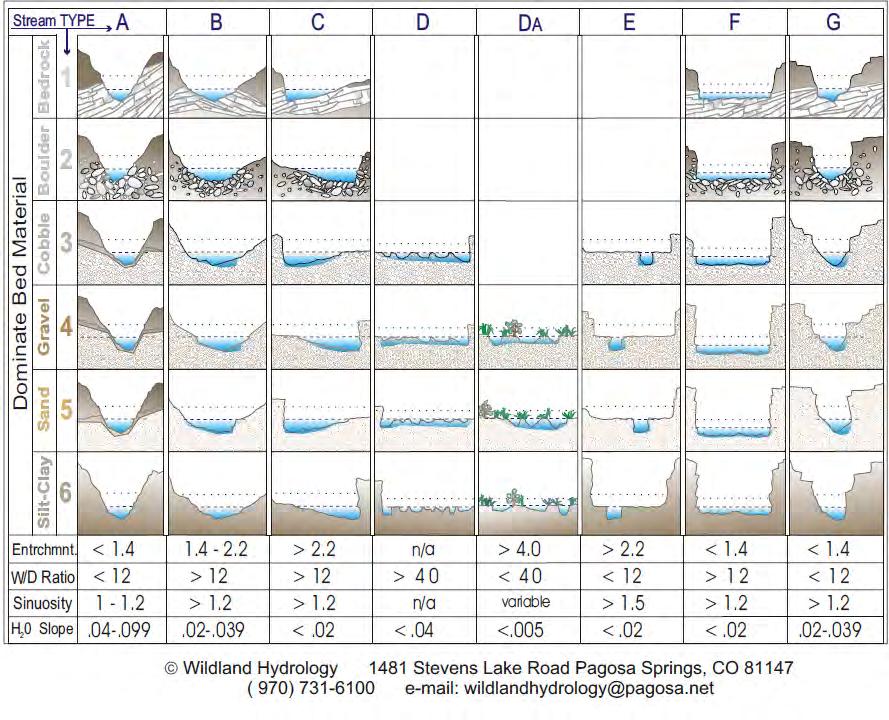
9 abandonment. In the San Francisco Bay Area many channels have adjusted to legacy and modern land use practices by increasing their peak flows, incising their streambeds, and abandoning their floodplains. Incised alluvial channels have a central tendency to form a new inner bench floodplain within their terrace banks. During large floods, such incised natural channels will generally not achieve long-term stability until sufficient floodprone width (above the level of the floodplain) has been gained through terrace and bank erosion. Although different definitions of floodprone width are possible, the definition used here is the quantitative expression used by Rosgen (1996): the width measured at twice the maximum bankfull depth An additional channel metric that is important to understand when evaluating channel stability is the entrenchment ratio. It is the ratio of floodprone width to bankfull width. It is used as by Rosgen in his Stream Classification System where channels that are slightly entrenched have an entrenchment ratio of 2.2, moderately entrenched have a ratio of 1.4 to 2.2, and highly entrenched channels have a ratio less than 1.4 (Rosgen, 1996). Rosgen considers that highly entrenched channels on valley floors with stream gradients less than 4 percent tend to be unstable. These channel types are called F and G channels depending primarily upon their entrenchment ratio and width/depth ratios. A graphic example of the Rosgen Stream Classification system is located in the Appendix B. It is important to note that an incised channel is not necessarily highly entrenched or unstable. A channel can be deeply incised into its valley floor but still have developed sufficient floodprone and bankfull width to attain stability. Within incised channels, the inner floodplain bench may only be a relatively shortterm feature until sufficient adjustments in hydraulic geometry have been achieved to create a broad enough floodprone width to pass the largest floods without continued adjustment. This is why the floodprone width, not just bankfull width, is an essential design parameter for stream restoration. There may also by cycles of channel adjustment due to episodic events of very high recurrence interval floods that exceed the elevation of floodprone width, such as from El Nino events, or have very high sediment loading from landslide producing storms. The amount of time required for a channel to attain stability, where a very large flood won t cause a change in cross sectional area or floodplain abandonment could be considerable, in the tens to hundreds of years. Given current influences of land use impacts and a changing climatic regime, we suggest that floodprone width should be considered in all restoration and channel stability evaluations. 7

10 MARIN AND SONOMA COUNTIES REGIONAL CURVES REPORT Bankfull discharge Figure 1: Flood frequency and sediment discharge are graphed to show effective and bankfull discharge. From Wolman and Miller, Figure Figure 2: 2: A A natural natural river river is at shown bankfull to be flow. flowing at bankfull stage. 8

11 Figure 3: Schematic cross section of a river showing bankfull depth. From Rosgen, Figure 3: Bankfull stage dimensions are shown in this schematic cross-section of a river (from Rosgen 1996). 1.2 Background to Hydraulic Geometry and Regional Curve Analysis Consistent and accurate identification of bankfull stage in the field is an important tool for managers, landowners, and stream practitioners involved in restoration design and bank stabilization projects. It was therefore the primary focus of this field study. Regional curves are a power law curve fit for plots of measured estimates of bankfull width, depth, cross sectional area, and often discharge plotted against drainage area. Drainage area can be easily measured from maps to predict one or more of these parameters. Figure 4 shows an example of hydraulic geometry curves for various western regions including the San Francisco Bay Area curve developed by Dunne and Leopold (1978). Dr. Leopold and his collaborators developed and published regional curve data in the 1960s and 1970s for a variety of locations around the United States. Regional curve plots for bankfull flow, width, depth and crosssectional area were plotted against drainage area for several locations including the San Francisco Bay Area curve for 30-inches of rainfall. Figure 4 indicates that variations in stable channel dimensions exist regionally, but because we cannot see the data points it is not possible to view the range of variation of local streams for a single region. Leopold s single Bay Area regional curve does not show the 9

12 MARIN AND SONOMA COUNTIES REGIONAL CURVES REPORT scatter of data about the trend line or stratify the data to account for the wide variability in rainfall and geology. For the original Leopold expression of hydraulic geometry sees Appendix A. Based upon some original data tables that Leopold used for developing several curves we have been able to determine that his technique for determining bankfull parameters was based upon flood frequency analyses of USGS gage sites and not based upon field surveys of floodplain benches. It appears that for the San Francisco Bay Area regional curve, Dr. Leopold selected the 1.5 year recurrence interval to establish the expected bankfull discharge and hydraulic geometry parameters. Our approach differed in that we developed our regional curves based on determining bankfull parameters from field surveys. We believe this to be a better approach for developing regional curves intended for use in creek restoration design projects that rely on bankfull geometry rather than on flood frequency estimates. We also expect that field conditions should reflect possible changes in discharge that have been brought about by legacy and modern land use practices. We do not know which specific streams or how many sites were used by Leopold, but the label on his curve is for an average rainfall of 30 inches. From reviewing the data tables we surmise that 30 inches was the average amount from all the gage sites he analyzed. Regional curves are central to the ecological restoration design process, as well as sustainable channel management. A number of approaches to creek assessment and restoration design have been developed that utilize regional curves as integral to channel design to foster natural creek functions that provide for stable and therefore relatively sustainable sediment transport, flood conveyance, aquatic habitat, and riparian development. The regional design curves provided under this project provide hydraulic geometry design curves from channels that were sought to represent a variety of field conditions. Although not all channels had stable sites, an effort was made to seek reaches with the least amount of active erosion and perform enough reconnaissance to identify various bankfull stage indicators representing the floodplain bench or its incipient formation. Identifying inner floodplain benches within unstable channels is challenging at the best, but with regional curves as an additional tool, we believe that this information will help guide other engineers, geomorphologists, landscape architects and planners involved in creek restoration design or stream network analyses. We additionally used the Rosgen Stream Classification system, described in applied River Morphology (Rosgen, 1996), to identify the stream stability classes of our survey sites. This information provides an independent but additional evaluation tool to assess the status of the sites that we used to construct the regional curves. 10

13 Figure 4: Original Leopold Regional Curves (1978) for bankfull dimensions versus drainage area (reprinted from Rosgen 1996). The San Francisco Bay Area curve is shown as line A in blue. 11

14 MARIN AND SONOMA COUNTIES REGIONAL CURVES REPORT In our experience, many poorly functioning or failed restoration projects are caused by failure to build appropriate channel dimensions, especially for both the bankfull and floodprone width. Floodprone width might be one of the most overlooked components in hydraulic geometry analyses and restoration design. Poor choices in channel dimensions in the design of restoration projects can lead to a cycle of unanticipated channel adjustments that can lead to landscape instability, costly repairs, and problems of excessive sedimentation or erosion, as well as diminished water quality and aquatic habitat. By focusing data collection in two counties with similar hydro-geomorphic provinces, this project attempts to expand and improve upon the original San Francisco Bay Area Regional Curve developed by Dr. Luna Leopold prior to the 1970s. Regional curves are being developed around the country. Examples of other areas conducting regional curves projects can be found at the NRCS website: Study Limitations The bankfull regional curves presented in this report are applicable to the field identification of bankfull geometry and discharge in non-tidal reaches of streams within Marin and Sonoma Counties. The impacts of urbanization and land-use activities over the last two centuries have altered the natural geometry and channel equilibrium in many of these streams. Indeed, most of the channels located at USGS stream gage sites have water impoundments and diversion operations upstream of the gage sites. These counties have sufficient open space areas and relatively low density development that we were able to access and survey adjustable alluvial channels that under a variety of geology, topography, and adjacent land use practices. The factors that influence creek channel morphology have not been fully evaluated in Bay Area streams. Bankfull discharge and its hydraulic geometry environment should not necessarily be considered static. It should be periodically reassessed through field surveys that will reflect a complex, dynamic and potentially changing relationship of a stream working to develop equilibrium with its imposed hydrology and bedload transport requirements. Typically, our large to moderate sized watersheds have constant perturbations imposed by modern land use. Constraints such as these should be considered when assessing the applicability of these regional curves. These curves cannot replace the need to collect original data at any stream restoration project. Streams included in this study varied greatly in how easily identifiable the bankfull characteristics were in the field. Many of our creeks are actively incising, creating episodic cycles of incision often initiated by moderate to large flood events and probably associated with both land use and climate change. When performing geomorphic field surveys within incised creeks, bankfull elevation can often be difficult to identify if a floodplain bench is not present. Therefore, additional field 12

15 indicators and lines of evidence of bankfull parameters were used wherever possible. These limitations are discussed in further detail below. 2.0 DATA COLLECTION METHODS 2.1 Site Selection Methods An initial goal of the project was to collect data at a range of stable creek sites across the two Counties. Given that many (if not most) creeks in these areas are in the process of adjusting their hydraulic geometry to land use changes, it was often difficult to find stable sites in places where access was assured. Once a stream area was selected, reconnaissance could often take half a day to just find a site that had a minimal amount of active erosion, no structural impacts, and where bankfull could be estimated. Although we tried to pick the most stable site within the available stream reach, not all sites could be considered to represent long-term stability. Because the Rosgen Stream Classification was used, we could apply the quantitative metrics of this classification system to identify which stream sites would be considered most stable within the classification scheme. Whether or not this system is used by others, the metrics are reproducible quantitative measures that can improve our understanding of channel conditions. Field sites were selected by identifying reaches with the following characteristics: o Sites showing channel characteristics that had stable conditions wherever possible, but in their absence, sites that had the least evidence of active erosion from incision or bank widening within the reconnaissance area. o Public lands or sites where permission to access was obtainable. o Non-tidal conditions, no structural influences unless at an actively operating USGS stream gage site. o A stream reach exhibiting consistent bankfull elevation relative to the stream bed over a length of approximately seven bankfull channel widths. Data was collected over a range of elevation, stream order, and mean annual precipitation, and geomorphic conditions. Figures 5 and 6 show the location of field sites in Marin and Sonoma Counties, respectively Field Data Collection Methods Fieldwork involved completion of a field data form (developed specifically for the project), survey of at least one cross section, survey of the longitudinal profile through the cross section, a pebble count and measurement of protrusion heights of large cobbles or boulders, if warranted at each cross section. Field data were 13

16 MARIN AND SONOMA COUNTIES REGIONAL CURVES REPORT collected between 2009 and 2011 for the purpose of computing bankfull geometry and discharge. A reconnaissance survey was performed at each site until a suitable cross section and longitudinal profile site could be found. Because these computations are based on the relative elevation of the bankfull channel, data collection was focused on identification and surveying of bankfull features. Before surveying, but after the reconnaissance survey to select a reach to survey, the field team often re-walked the reach of interest a distance of at least 5 to 7 times the estimated bankfull width, upstream or downstream from the cross section site, to identify potential morphological features representing bankfull stage. This distance represented the minimum distance of all the longitudinal profile surveys. When bankfull conditions were difficult to determine at one cross section or when two sites presented differing conditions of width/depth ratio and entrenchment ratio (floodprone width divided by bankfull width), but had obvious bankfull indicators, an additional cross section would also be surveyed. The width/depth ratio and entrenchment ratio are also the primary metrics used in the Rosgen Stream classification system for identifying stable and/unstable conditions. For surveying the cross sections and profiles and conducting the pebble counts, we generally followed the methods outlined in the USDA s Stream Channel Reference Sites: An Illustrated Guide to Field Techniques (Harrelson, Rawlins and Potygundy, 1994).Specific field surveys conducted include the following: Bankfull Stage Longitudinal Survey A survey of field indicators for bankfull stage was conducted at each location for at least the length of 5 to 7 bankfull widths. The field indicators of bankfull stage typically included the following and all were used in tandem to represent lines of evidence of bankfull elevation: o Depositional features that can sometimes represent the floodplain, including adjacent relatively flat bench that has consistency on either side of the channel, topographic breaks in the bank, top of point bars and/or short, alternating lateral bars with consistent elevational gradient along the reach; o Consistency of bankfull stream gradient with surface water gradient along the length of the reach. When available, knowledge of the last peak discharge and the high water mark was used to establish whether it was above or below bankfull stage to help establish the bankfull elevation; 14

17 o Changes in particle size along the cross section. Commonly smaller particles deposited from suspension are found on the floodplain than in the channel bed or banks, but special circumstances can produce the opposite; and o Consistency of riparian elevation, however, some species can often grow below bankfull stage. Thalweg and Water Surface Longitudinal Survey The elevation of the streambed thalweg that best defined the sequences of riffles, runs, pools and glides, as well as water surface, high water marks, and bankfull were surveyed to establish the riffle head features and to best determine the bankfull stream gradient from estimates of both the bankfull stage survey and the riffle head to riffle head gradient from the thalweg survey. Cross-Section Surveys - One to two cross-sections were surveyed by level at locations along the profile where the creek showed the best-defined bankfull characteristics and the greatest stability relative to site conditions. Cross section surveys were extended above the floodprone width wherever possible to exceed the floodprone height. Pebble Counts Wolman pebble counts were conducted at each crosssection and plotted to develop the various particle size distributions for the bed surface at each section as well as noting the largest particle in the cross section. In particular, the d50 and d84 particle sizes were developed and tracked per cross section. Average Protrusion Height - In boulder-influenced streams, we measured the average protrusion height to refine estimates of hydraulic roughness using empirical formulas. Miscellaneous Other Observations Numerous other observations and measurements were collected and recorded and will be used at the next phase of data analysis. These observations include the percent fines (<2 mm) in the channel banks (visually estimated) as well as notes to the following: o Bank strength (as noted above the percent of silt-clay [cohesion] in channel banks/bed (visual estimation)) o Percent of vegetation density and classes o Assessment and measurement of large woody debris in the channel (especially important in wood dominated systems) o Historical land use influences o Local geology 15

18 MARIN AND SONOMA COUNTIES REGIONAL CURVES REPORT o Bed morphology o Qualitative assessment of current dominant sediment source to reach o Visual estimate of dominant bed sediment class o Dominant geomorphic setting i.e., alluvial fan, narrow alluvial valley floor, low gradient wide alluvial valleys, narrow colluvial valley floor, generally high gradient canyons dominated by bedrock control in channel bed o Historical changes in Rosgen Stream Classes o Observations of the amount of historical incision occurring All field data were entered into an Excel spread sheets to develop a matrix of all stream parameters. 2.3 GIS Data Analysis Methods Some parameters were not measurable in the field and were measured by using a Geographic Information System (GIS) database. Staff at the San Francisco Estuary Institute (SFEI) made these measurements by using ArcGIS Many of these values may be used in future Phase 2 analyses that will involve stratifying the regional curves by different parameters. The measurements included the follows items: Drainage Area (square miles) Drainage areas were calculated in ArcGIS using the BAARI streams and NHD flowline databases brought into a 10m Digital Elevation Model (DEM) by first calculating flow direction and flow accumulation, snapping the pour point to the cell of highest flow accumulation, running the GIS watershed tool, and calculating total watershed area. Upstream Drainage Network Length (feet) SFEI used BAARI streams upstream of point (using watershed boundary) and calculated sum of length. This analysis included mapped culverts. The flow lengths are summed lengths of all BAARI streams within the modeled watershed area. SFEI calculated the percentage of lines within drainage areas that were classified as culverts, and it was typically very small (~0.5%). Drainage Density (miles/square mile) Drainage density is the linear feet of channel network as determined by GIS measurements described above divided by the watershed drainage area. It is a measure of the degree of channelization in the watershed and therefore reflects natural variation caused by different geologic and climatic settings. It can also provide an indirect measure of changes from urbanization when ditches and storm drains are included in the analysis. 16

19 Drainage Area above Dams for USGS gage sites (square miles) SFEI used drainage area procedure at dam points to develop the drainage areas above the dams. These areas were subtracted from the total drainage area to provide a better estimate of contributing drainage area for bankfull flow at the surveyed gage sites. Impervious Surface (percent impervious) - National Land Cover Database (NLCD) Impervious Surface grid for year 2006 was used to perform Zonal Statistical analyses. Precipitation (inches) - The precipitation was based on the Oregon State PRISM average precipitation for the period of to develop the mean annual precipitation (MAP) values at each specific survey sites. Note that the PRISM is generated at a fairly coarse scale using available rainfall data (but certainly not all rainfall data) and applying statistical methods. The MAP results may not be as accurate as specific site-specific raingage data (if available), but for consistency PRISM MAP values were used for data analysis at all sites. Vegetation Acreage (square meters) The CalVeg dataset (USFS) 2002 and 2003 was used and a clip on each drainage area was performed to develop vegetation acreages. 2.4 Bankfull Discharge Calculation Methods To calculate bankfull discharge, measured field parameters were entered into a spreadsheet called STREAMS (Mecklenburg 2006), which was specifically developed for analysis of fluvial-geomorphic data. Estimates of bankfull discharge assisted us in determining whether we had picked a reasonable elevation for bankfull stage, as well as providing us the opportunity to plot a regional curve of bankfull flow. Various hydraulic parameters were calculated from riffle slopes plotted independently in excel spreadsheets. Width/depth and Entrenchment ratios, pebble counts, and stream gradient were also used to classify channel stability as per the Rosgen Stream Classification system (Rosgen, 1996) and to stratify the data per stream class at a later Phase 2 of the project. For each data collection site, except for the USGS gage sites where recurrence intervals could be determined, the following parameters were used in the STREAMS spreadsheet to calculate bankfull discharge: Mean bankfull depths (D bkf) Maximum bankfull depth (D max) (to determine height to measure floodprone width) Channel slope (S bkf) (bankfull gradient determined from thalweg longitudinal profile from riffle head to riffle head and/or bankfull stage survey) 17

20 MARIN AND SONOMA COUNTIES REGIONAL CURVES REPORT Bankfull width (Wbkf) Floodprone width (Wfpa) (measured at twice maximum bankfull depth) Bankfull flow (Qbkf=Vbkf*Abkf) (calculated from measurement of stream slope and equations for Manning s n values) (A is area = W bkf D bkf) Wetted perimeter (P) ~ 2 *Dbkf + Wbkf (used to determine hydraulic radius) Hydraulic radius (R) = Abkf/P (P= wetted perimeter) Roughness/friction factor/manning s n values under bankfull flow conditions = R 1/6 /(U/U*)g 1/2 (where U/U* = relative roughness and g = gravitational acceleration] Velocitybkf (estimated from Manning s equation Vbkf = R 2/3 S 1/2 /n) Bed sediment sizes (d50/d84) from pebble counts Various Rosgen stream typing parameters including the following: o Width/depth ratio (Wbkf/Dbkf) o Entrenchment ratio (Wbkf/Wfpa) Bankfull Flow Recurrence Interval - At field sites located near a USGS stream gage station, the longitudinal profiles and cross-section bankfull elevations were used to select or evaluate the bankfull stage at the streamflow-gauging station. In some cases the gage elevation was tied into the survey allowing the bankfull elevation to be compared to the stage-discharge relation developed by USGS for the gage site. At other sites we developed a flood frequency relationship and looked for indications of the rate of increase in discharge slowing as flow spilled onto a bankfull bench and used this value to determine which inner bench represented bankfull discharge at some of the more difficult sites that were influenced by upstream dams. The recurrence interval of each bankfull discharge was determined from a frequency distribution of annual peak discharges following methods described in Bulletin 17B. 3.0 RESULTS 3.1 Field Site Characteristics This section summarizes the broad characteristics of the survey sites. There were a total of 57 cross sections surveyed at 45 different field sites. Marin had 32 sites and Sonoma had 13. Many parameters could be used to characterize the various survey sites, but the following five were selected as readily available and easily understood metrics to provide a basis for expressing the range of site conditions. Figure 5 and 6 show the locations of the field sites in Marin and Sonoma Counties. 18

21 Figure 5: The map shows the locations of Marin County Survey Sites. San Antonio Creek straddles the Marin and Sonoma County line. 19

22 MARIN AND SONOMA COUNTIES REGIONAL CURVES REPORT Figure 6: The map shows the locations of Sonoma County Survey Sites. Table 2 (page 39) shows the list of sites surveyed as part of this project along with some key parameters. The streams in this study are single-channels with slopes ranging from 0.12% to 9.5%. More details on site characteristics are described below. The data is presented in plots of frequency distributions which are simply counts of the number of data points (sites) that are within the specified parameter range. For example, Figure 7 shows the number of field sites (the total columns in blue) within each specified range of slopes. These types of plots provide information on the range and characteristics of the project field sites. Range of channel slope (gradient) Channel slopes in the dataset ranged from 0.12% to 9.5%. The majority of slopes were in the 1% to 1.5% range and under but there were 8 sites with slope greater than 4%, which is often considered the slope range for steeper channel morphologies such as step-pools and cascade type channels. There were 2 sites at slopes greater than 6 percent, which are steep enough to be influenced by debris flow processes. As shown in Figure 7, about 59% of the sites have channel slopes less than 1.5%. 20

23 Frequency Distribu/on of Field Sites by Channel Slope Class Total % 0.5%- 1% 1%- 1.5% 1.5%- 2% 2%- 3% 3%- 4% 4%- 5% 5%- 6% 8%- 9% 9%- 10% Figure 7: The graph shows the frequency distribution and number of field sites by channel slope class. Drainage Area Drainage areas varied from 0.02 mi 2 to 50 mi 2 with the majority of sites at 5 mi 2 or less. Shown below in Figure 8 is a frequency distribution of number of sites in each drainage area class. About 63% of the sites had drainage areas less than 5 mi 2. Frequency Distribu/on of Field Sites by Drainage Area Class <1 mi2 1-5 mi mi mi mi mi2 Total Figure 8: The graph shows the frequency distribution and number of field sites by drainage area class. 21

24 MARIN AND SONOMA COUNTIES REGIONAL CURVES REPORT Dominant Geomorphic Setting - For each site, the dominant geomorphic setting was noted in the field. These setting are based on local observations from the field site and not from extensive mapping. About 35% of the sites were in a wide alluvial valley, 22% were on alluvial fans. Figure 9 shows the frequency distribution of field sites by dominant geomorphic type. The categories of dominant geomorphic setting are as follows: Type 1. Wide alluvial valley, >5 W bkf Type 2. Narrow predominantly alluvial valley, <2 W bkf Type 3. Moderately wide alluvial valley, 2-5 W bkf Type 4. Alluvial fan Type 5. Narrow, predominantly colluvial valley or canyon Type 6. Steep, mostly bedrock confined canyon Type 7. Plain, often uplands transitional to tidelands 25 Frequency Distribu/on of Field Sites by Dominant Geomorphic Type Total Type 1 Type 2 Type 3 Type 4 Type 5 Type 6 Figure 9: The graph shows frequency distribution and number of field sites by dominant geomorphic type. Mean Annual Precipitation Mean annual precipitation (MAP) values were developed from the Oregon State Precipitation PRISM project and ranged from 30.8 to 53.6 inches per year of rainfall. This fairly large variation in MAP over this relatively small area is typical of the orographic effects of the Pacific Ocean and the mountainous terrain of Marin and Sonoma Counties. The combined average rainfall for the sites is inches. The average rainfall for the sites reported by Leopold was 30 inches. We expect that the methodologies of determining average 22

25 rainfall are different for the two regional curves. More precipitation data is now available throughout various watersheds than was available during the 1970s when Leopold constructed his San Francisco Bay Area Regional Curve, but we also expect that many of our sites are located in more upland topography, where rainfall tends to be greater than the primarily lowland USGS gage sites evaluated by Leopold. Rosgen Stream Type The Rosgen (1996) Stream Classification System was used to classify the various stream types as shown below in Figure 10. Note that for three sites a modified Rosgen classification system was used that allowed the width/depth ratio to vary by +/- 3, instead of the usual spread of two, and for the classification system s threshold of 12 to be changed to 10 for a few of these sites. This adjustment was based on previous discussions with Dave Rosgen and experience applying the system in the SF Bay Area (Rosgen personal communication 2002). Note that there were two very small streams in China Camp that did not classify under the modified Rosgen system. One site was on an alluvial fan along a losing reach (reach of stream that loses surface flow to groundwater) and the other was in bedrock. The frequency distribution shown below of number of field sites per Rosgen Stream Class indicates that the majority of sites classify as a Rosgen B type with entrenchment ratios that range from 1.4 to 2.2 (+/- 0.2) and a W/D ratios >12 (+/- 2). A classification breakdown that identifies the stream sites relative to their classification and which were classified using the modified Rosgen system is provided in Table 2 (page 25). Figure 10: The graph shows the frequency distribution and number of field sites by Rosgen Stream Class. 23

26 MARIN AND SONOMA COUNTIES REGIONAL CURVES REPORT The sites that are classified as F or G type streams are considered unstable in the Rosgen Classification system. These surveys were from sites that did not have any identifiable stable reaches in the field. As a result, for these stream classes (F and G), we feel that bankfull cross sectional area (width times depth) is the most reliable metric from a regional curves, rather than relying on width or depth for developing stable channel geometry. We included these channel types because in Phase 2 of our project we hope to stratify regional curves by stream type to see if differences in width and depth of stable channels can be statistically detected. Without this kind of stratification, it is difficult to determine from any regional curve what the channel stability conditions were for particular sites or to assess the impact of these sites on the curve regression results. 3.2 Regional Curves of Bankfull Conditions This section presents the results of the first phase of data analysis covered under project funding. The terms of the original EPA grant that partially funded this study require regional curve plots of only bankfull width, depth and crosssectional area as a function of drainage area (Figures 6-8). In addition, to these plots, we have also included several other plots of various data parameters along with our initial interpretation. The next Phase 2 of data analysis, given additional funding, will include a more in-depth stratification of data by different parameters, including Rosgen Stream Class. We hope to improve correlation and explain causation of the variation in data to better assess influences on bankfull channel geometry, especially as it relates to relative stability. Comparison with the Original Leopold Regional Curves As discussed earlier, Leopold appears to have developed his San Francisco Bay Area Regional Curve by performing flood frequency analyses to determine the discharge associated with the1.5-year recurrence interval of streams gaged by the USGS. If true, our field based method differs substantially than the flood frequency analysis method used by Leopold. Leopold felt that the 1.5 year return period best represented the average bankfull discharge that was reported at the time to commonly occur between 1.3 and 1.7 years. Table 1 shows our field-based estimates of the recurrence interval of bankfull discharges at five USGS gage stations that we assessed. Note that all, except the Sonoma Creek gage site have significant upstream water diversions reservoirs that have all been in place longer than 50 years. We believe that enough time has passed to provide sufficient field indications of bankfull discharge at the gage sites that can be calibrated through flood frequency analyses that includes the influences of the dams. At the gage sites bankfull discharge ranged from a recurrence interval of 1.1 to 1.5 years. The one site that had a recurrence interval of 1.5 years was Walker Creek, which has the least urban impacts of the five sites but a long history of grazing usage. We believe that the lower estimates of 1.1 to 1.3 are in keeping with recurrence intervals from other urbanized and altered watersheds that have increased peak flows caused by urban runoff and increased drainage density (the latter is increased by artificial channels such as ditches and storm drains). 24

27 Table 1: Calculated Recurrence Interval for Bankfull Discharge at Gage Sites Site Corte Madera Creek at Ross, Gage Site Lagunitas Creek at Samuel P. Taylor Park, Gage Site Novato Creek at Novato, Gage Site Sonoma Creek at Agua Caliente, Gage Site Walker Creek near Marshall, Gage Site Bankfull Discharge (cfs) Reservoir Upstream Approximate Recurrence Interval (years) 953 Yes Yes Yes No Yes 1.5 Note: Recurrence intervals were determined from a flood frequency analysis of Peak Annual flows from USGS data. Regional curve plots are provided in this section with the original Leopold curve added to our graphic plots for comparison purposes only. The location of the original Leopold line is drawn as close as possible to the published graph shown in Figure 4 but it was not derived by plotting Leopold s original data, since we do not know which gage sites were used. Also, Leopold s original regional curve did not extend to drainage areas less than 0.1mi 2. This is probably because USGS gage data were not available for such small streams. However, many creek restoration projects are constructed on these smaller streams and thus our regional curves help fill in data gaps for these smaller drainage areas. It is important to note that for sites with upstream reservoirs, we adjusted the drainage areas for the regional curves to exclude the area impounded behind the dams. We expect that this was not done for the Leopold curves. 25

28 MARIN AND SONOMA COUNTIES REGIONAL CURVES REPORT Figure 11 shows a strong relationship between bankfull cross sectional area and drainage area as indicated by the high R 2 value of shown in Figure 7. The difference with the original Leopold trendline is quite high especially at the smaller watershed drainage sizes. This pronounced difference especially for the smaller drainage areas, which is also seen for the other two plots of width and depth, may be the result not only of the different calculation methodology (1.5 recurrence interval versus bankfull field indicators), but also that Leopold s trendline is likely based on gaged sites that did not have drainage areas smaller than 0.1 mi 2 and likely included the drainage area behind dams for sites that had upstream reservoirs. We consider the regional curves of cross sectional area to be the most useful curve compared to width or depth because cross sectional area tends to reduce the influence of local variations associated with differences in the width/depth ratio. On the other hand, the plots showing width and depth are independently more likely to indicate a stronger signature and influence of channel stability if data were stratified by width/depth ratio, entrenchment ratio, and Rosgen Stream Classification which combines the two ratios, among other things, into stream classes. This hypothesis would be further tested in Phase 2 if funding is available. Figure 11: The plot shows the relationship between bankfull cross-sectional area and drainage area for streams in Marin and Sonoma County field sites. 26

29 Walker Creek Data points (discussed below) Figure 12: The plot shows the relationship between bankfull width and drainage area for streams in Marin and Sonoma County field sites. In addition, we expect that a number of gaged streams evaluated by Leopold had their width and depth artificially influenced by instream structures, such as weirs or bridges, since many gage sites tend to be associated with these controls. Figure 12 shows a strong relationship between watershed area and bankfull width as indicated by the R 2 of Again the difference between our results and the original Leopold results is most pronounced for smaller drainage basins. As can be seen in the plot a broad variation in channel width can occur as shown for the widest three data points for the same channel at cross sectional area of 12.6 ft. Although the cross sectional areas have a very small range, the bankfull widths for three cross sections on Walker Creek range from 55 to 80 ft (as shown in figure 12 at the 12.6 mi2 drainage area), and the site with the widest bankfull width is the one considered to have a more stable form relative to the Rosgen Stream Classification that indicates that the wider channel is a B type channel as opposed to an F at the two other narrow sites. The narrower sites are more unstable because their width depth and entrenchment ratios are low and their floodprone widths are too narrow relative to their bankfull widths. This demonstrates the value of the next step in Phase 2 to stratify the data relative to stream type if additional finding can be secured. 27

30 MARIN AND SONOMA COUNTIES REGIONAL CURVES REPORT Figure 13: The plot shows the relationship between bankfull depth and drainage area for streams in Marin and Sonoma Counties. Figure 13 shows that the correlation between watershed area and bankfull mean depth is also statistically strong across the range of drainage areas as indicated by the R 2 of As described above, the difference in results is most pronounced at the smaller drainage basins. The implication of the differences in the trend lines for stream restoration projects is the potential of designing stable channels versus ones that could have inherent instability because the width depth ratio is too large or too small. If one relied on regional curves that are derived from uniform flood frequency recurrence intervals, such as that derived by the Leopold curve, then the bankfull depth relative to bankfull width could lead to designing entrenched channels. For example, for a channel of a 1 mi 2 drainage area, the bankfull depth based upon our field derived regional curve should be about 1.1 ft. From Figure 12 the width should be about ft, providing a cross sectional area of about ft 2. This would provide a width/depth ratio of Alternatively, if the width and depth were derived from the Leopold curves, 17 ft and 1.55 ft would respectively provide a cross sectional area of about 26.3 ft 2. The width/depth ratio would still be 11.0 but the cross sectional area of a design channel would be too large, leading to an entrenched condition that if applying the Rosgen Classification System, would create an unstable F or G channel. 28

31 Figures 14 and 15 both show the correlation of floodprone width against drainage area. However, Figure 14 includes the correlation of all the data but also shows the unstable G and F Rosgen Stream Classes plotted as light yellow markers. For this graph the R 2 value of is lower than that for Figure 15 that has an improved R 2 value of because it correlates the data without using the unstable and therefore aberrant G and F data. These graphs demonstrate the importance of understanding channel stability conditions when using or developing regional curves. As an example to illustrate the importance of using the proper curve for creek restoration design, if the floodprone width were determined for a channel with a 1 mi 2 drainage area from the two different plots in Figures 14 and 15, the respective widths would be 23.7 ft and 26.1 ft. If the entrenchment ratio for the channel was determined, the floodprone width would be divided by the bankfull width of 12.89, equaling either 1.8 or 2.02 depending on Figure 10 or Figure 11. With a width/depth ratio of 11.7, the Rosgen Stream Class would be designed for a relatively stable B Stream Class, which are defined by entrenchment ratios ranging from 1.4 to 2.2 +/- 0.2 and width/depth ratios greater than 12 +/ As can be Figure 14: The plot shows the relationship between floodprone width and drainage area for streams and Marin and Sonoma Counties. The yellow data markers indicate unstable conditions observed in the field for Rosgen Stream Class F and G channels. 29

32 MARIN AND SONOMA COUNTIES REGIONAL CURVES REPORT Figure 15: Plot shows the relationship between bankfull floodprone width and drainage area for streams in Marin and Sonoma Counties. Unstable streams of Rosgen Stream Class F and G have been removed from this analysis. seen, the predicted width/depth ratio of 11.7 is close to the threshold of stability. We expect with improved refinement and stratification of regional curves data for width and depth, better predictions of stable hydraulic geometry could be derived. Note that we are not aware of a regional curve for flood-prone width for the Bay Area, nor have we seen this parameter developed for other regions. If the data were stratified based upon Rosgen stream classes, we expect that there could be stronger correlations within each of the Rosgen stream types, but clearly the most stable stream types would be of interest for restoration design. If correlations are good for stable versus stable Rosgen stream types, it might be possible to use stratified regional curves in the future to assess the potentially stability of a site just by knowing its drainage area and bankfull width. Since there are several channels that have unstable G and F Rosgen Stream Classes, if the data were stratified by stream type we would expect to see some strong relations with larger floodprone widths for the more stable channel types. 30

33 Figure 16: The plot shows the relationship between of bankfull flow and drainage area for streams in Marin and Sonoma Counties. Figure 16 shows the results of the best fit trend line for bankfull flow versus drainage area. It has an excellent correlation coefficient of R 2 = for the relation between the calculated bankfull flow versus drainage area. The calculated bankfull flow curve agrees fairly closely with the Leopold curve that was developed using the 1.5 year recurrence interval flow for gaged streams. This might indicate that as urbanization influences and peak flow have increased, perhaps even due to increased rainfall since the 1970s, bankfull discharge has not significantly changed but its frequency has increased. The ratio of mean depth to maximum depth is a non-dimensional metric representing the shape of the channel. Higher values are indicative of more rectangular shaped channels; a value of 1 representing a perfect rectangle. Figure 17 shows lower values represent more triangular channel shapes. The slope of the best fit line approximates During Phase 2 we would expect to see distinct patterns relating to channel stability, especially if additional data were collected on all stream types to create a valid, statistically large data set, combined with this existing data set, and all stratified by Rosgen Stream Classes. 31

34 MARIN AND SONOMA COUNTIES REGIONAL CURVES REPORT Figure 17: The plot shows the relationship between mean depth and maximum max depth. This relationship can be used in the field to estimate mean depth. The mean depth would be attained by multiplying the maximum bankfull depth by and adding (the Y-intersect of the best fit line). The estimated mean depth can be multiplied by the measured channel width to estimate cross-sectional area. If this plot was stratified to represent which channels were stable we expect that a higher correlation coefficient would be achieved and therefor designs for restoration projects might be guided toward designing a more stable channel form. A plot of Manning s n by Rosgen stream type is shown in Figure 18. Manning s n is a commonly used factor that represents the degree of hydraulic resistance to channel flow. Manning s n involves all forms of resistance including bank and bed forms, and vegetation into one factor. For this project, Manning s n values were calculated using a version of the Manning-Strickler empirical relations that estimate n values from the d50 or d84 grain size. Note that there are other approaches to calculating Manning s n values that will be further developed in Phase 2 of the project, if funded. For this project, Manning s values were calculated by the STREAMS program and the values shown in Figure 18 were all calculated using the same approach. As would be expected, the results show that the higher gradient (steeper) stream types (the Rosgen A or Ba channels) tend to show higher Manning s n values. Please refer to Appendix B for the Rosgen Stream Type table. 32

35 Figure 18: The graph shows Manning s n for the different Rosgen Channel Stream Classes. Figure 19: The plot shows the relationship between bankfull mean velocity and drainage area for streams in Marin and Sonoma Counties. 33

36 MARIN AND SONOMA COUNTIES REGIONAL CURVES REPORT Mean bankfull velocity was calculated using the bankfull flow value divided by bankfull cross-section area. Since bankfull flow is calculated by Manning s equation using the calculated Manning s n values described above, this estimate of bankfull velocity is approximate but was consistently developed across the range of sites. As sown in Figure 19, the statistical correlation was fairly poor (R 2 = ) which may reflect how the values were calculated or that additional data stratification is required. If funded, other variables or combination of variables (such as slope-area products) will be analyzed to see if they are statistically more predictive. Although regional curves use drainage area as a predictor of hydraulic geometry, we questioned whether drainage area would be the best or only predictor of these parameters given that many changes in the stream network have probably caused bankfull conditions to change since the 1970s when the Leopold Regional Curve was developed. Although the drainage area in many cases is still the same, the stream network and its drainage density has often been substantially altered, for example through headward erosion of first order tributaries, by ditching, by connecting channels that were previously disconnected from mainstem channels (often by alluvial fans at the base of steep hillsides), and by extensive storm drains or agricultural tiling systems. Figure 20: The plot shows the relationship between drainage network length and bankfull cross sectional area for streams in Marin and Sonoma Counties. 34

37 The relationship of upstream channel network length to drainage area shown in Figure 20 has a high R 2 value of This plot shows the relationship of all the data points that had a densified stream network mapped by SFEI. Because the stream network mapping has not been mapped for several cross sections sites in northern Sonoma County, these data points were removed from this plot. The plot indicates that stream network length, when it includes culverts and ditches, is a very good predictor of bankfull cross sectional area and works as well as drainage area which had a similar R 2 of 0.96 We expect that in watersheds that have been highly urbanized, and when GIS tools are readily available to make this calculation, especially where there are intensive additions of storm drains, that drainage network length could become a better predictor of hydraulic geometry than drainage area. This will be explored more in a Phase 2 of the project, if funded. 4.0 CONCLUSIONS AND NEXT STEPS The results of this project demonstrate that the relationship between bankfull channel dimensions and watershed drainage area in the Marin and Sonoma Counties of San Francisco Bay Area is strong and therefore provides a strong basis for use in restoration design and channel management. The curves of bankfull cross sectional area developed by this project can be used by both designers and planners to help determine bankfull dimensions. Following further data analysis of the more stable channels surveyed under this project, we expect to show the dimensions of the floodprone width that will provide much improved conditions for channel stability that will help protect natural creek functions during flooding events. The existing graphs include a mix of channel conditions including several incised channels (classified as Rosgen F and G type channels) that are in the data set. The importance of creating the appropriate floodprone width is therefore likely of key importance to natural channel design. Regional curves are a useful tool in the design toolkit for restoration engineers, planners and fluvial-geomorphologists. However, as for any empirically derived dataset, care should be used when applying regional curves relationships outside of the limits of the original dataset. In addition, it is also important to look at the specifics of each project site and to utilize hydraulic models that analyze specific watershed and site scale processes that may impact channel dimensions. Regional curves are only one tool for the creek designer and manager, and all projects need to evaluate site-specific conditions using as many of the tools that can contribute to the assessment. Datasets such as regional design curves are best developed at the local watershed or larger County scale as done in this project for Marin and Sonoma Counties. Because design consultants typically lack pertinent data and funding for research, 35

38 MARIN AND SONOMA COUNTIES REGIONAL CURVES REPORT regional curves are not practically done as part of any one local or specific restoration project. The expense and time associated with extra data collection and analysis can often be prohibitive to some projects, especially smaller ones. There is a direct practical analogy of these curves to the development of rainfall intensityduration-frequency (I-D-F) curves that are produced by flood control agencies and provided to engineers working on county or district projects. Public works agencies typically do not expect each practitioner to collect and analyze the historical rainfall data for each project and then develop a unique set of I-D-F curves. Regional design curves for creek restoration exemplify this type of data set that is best developed on a regional level and then provided to the individual project designers. Given current influences of land use impacts and a changing climatic regime, we suggest that it is key to incorporate floodprone width into any channel restoration design that uses hydraulic geometry concepts. Next steps in the project development should include further stratification in Phase 2 and analyses of the data to look for causative controls on channel morphology. We would also be adding to our database of regional curve sites from other creeks in Marin/Sonoma Counties as well as from other Counties around the Bay Area. Additional funding will allow this work to proceed and the results would allow a more in depth analysis of the causative factors on stable channel geometry that would be useful across a broad spectrum of users. In particular, we propose that a Phase 2 for this project could potentially include the following key items depending on interest and funding: Expand our current database of 57 data points. We would perform field survey and develop stable channel characteristics at a range of both stable and at unstable sites. We will also be able to focus our additional data points at locations of interest to local, state and federal agencies, such as steep gradient systems or creek systems impacted by land use. Additional data points will allow us to stratify and statistically analyze the data with a higher degree of certainty. Further stratify the datasets to investigate the dominant controls and influences on channel morphology. For example: o Determine how watersheds with increased drainage density (from artificial channels such as storm drains and ditches) might compare to historical conditions and how that would influence bankfull channel geometry. o Stratify data by Rosgen Stream Classes and compare regional curves that include versus remove unstable stream classes of and G type channels. o Stratify data by geomorphic conditions, such as alluvial fans, versus confined and unconfined valleys, to determine if there are predictable or unpredictable metrics of bankfull geometry. 36

39 o Further stratify data by precipitation and geologic conditions to test for differences. Work with a professional statistician to perform a wider range of statistical analysis. Add a riparian vegetation expert top our team to develop a database of field indicators of the extent of flood plain on the landscape. This assessment is useful to groups seeking to develop a scientific basis for stream setback requirements. Our work is already being incorporated into a study of stream setbacks being conducted by the San Francisco Estuary Institute (SFEI). Develop the dataset to assess water quality impacts of sediment production from channel erosion as unstable channels adjust their form to achieve more equilibrium conditions. Prepare a formal methods and procedures guidance document that clearly documents the work performed and can assist others in collecting field data and developing regional curves in other areas around San Francisco Bay. Publish the findings in a refereed journal and prepare lectures of findings and applicability of stratified regional curves for creek restoration design and watershed analyses. 37

40 MARIN AND SONOMA COUNTIES REGIONAL CURVES REPORT 5.0 REFERENCES References used during preparation of this report include the following: 1. Dunne and Leopold, Water in Environmental Planning, Hey R.D., Thorne C.K., Stable Channels with Mobile Gravel Beds, Journal of Hydraulic Engineering 112(8), Knighton, A.D. Fluvial Forms and Processes, Edward Arnold, London Leopold, L.B. and Maddux, T. The Hydraulic Geometry of Stream Channels and some Physiographic Implications, US Geological Survey Professional Paper 252, Leopold, L.B., A view of the river. Harvard Press, Cambridge, Massachusetts. 6. Mecklenberg, D. STREAMS Spreadsheets, Version 4.3L, Ohio Department of Natural Resources, Parker G., P. Wilcock, C. Paola, and W. E. Dietrich, Quasi-Universal Relations for Bankfull Hydraulic Geometry of Single-Thread Gravel-Bed Rivers, Journal of Geophysical Research Earth Surface, November Parker G.P. Hydraulic Geometry of Active Gravel Rivers, Journal Hydraulic Division, ASCE Volume 105, Rosgen, D., Applied River Morphology, Wildland Hydrology, Pagosa Springs Colorado. 10. Harrelson, Cheryl C; C.L. Rawlins; and John P. Potyondy, Stream channel reference sites: an illustrated guide to field technique. Gen. Tech. Report RM-245. U.S. Forest Service, Ft. Collins, CO. 11. U.S. Geological Survey, Guidelines for determining flood flow frequency, Bulletin # 17B, Hydrology Subcommittee, Interagency Advisory Committee on Water Data, US Geological Survey, U.S. Department of the Interior. 12. Wolman, M.G., and J.P. Miller, Magnitude and frequency of forces in geomorphic processes. 38

41 Table 2: Site Characteristics Site Drainage Area (mi 2 ) MAP (in) PRISM data Rosgen Stream Class Slope d50 (mm) d84 (mm) BF Cross- Section Area (ft 2 ) Bankfull Width (ft) Mean Bankfull Depth (ft) Bankfull Flow (cfs) Bear Valley E Blackstone x-section B Blackstone x-section E4b Carriger creek upstream of grove A Carriger Creek lower fan C Carriger Upper Fan F3b Cascade Creek (Fairfax) x- section B3c Cascade Creek (Fairfax) x- section B3c Cascade Trib E4b Cheda Creek X- Section B4c Cheda Creek X- Section B4c China Camp Creek - Xsec A China Camp Creek - Xsec B4a China Camp Miwok Meadow South Trib N/A China Camp Gully North Fork N/A Corte Madera Crk at Ross Gage - Sec 1, modified F

42 MARIN AND SONOMA COUNTIES REGIONAL CURVES REPORT for upstrm dam Corte Madera Crk upstream of Ross gage - Xsec 3, modified for upstrm dam G4c Crane Crk at Regional Park C3b Deer Creek Lower Xsection B4c Deer Creek Middle B4c Deer Creek Upper E Devils Gulch, modified for upstrm dam F East Fork Olema Crk C Emu Trib of San Antonio Crk B4c Giacomini Trib E3b Graham Crk B3a Halleck Cr. Peekaboo F Lagunitas Crk SPT Park Sec 1 (not a riffle). Modified for upst dam C Lagunitas Crk SPT Park Sec 2 (riffle). Modified for upstrm dam B4c Unnamed Trib into Lagunitas Crk B Larkspur Creek B4c Miller Crk Marinwood B4c Miller Lucas Site B4c Miller North Fork B

43 Nicasio at Nicasio, modified for upstrm dam C Novato Crk Section 1, modified for upst dam G4c Novato Crk Section 2, modified for upstrm dam F4 (B4c) Olema Crk John West Fork B4c San Antonio Crk near Hwy 101 Sec F San Antonio Crk near Hwy 101 sec C Sausal Creek Sec 1 Sec F Sausal Creek Sec F Sleepy Hollow Creek, headward site, San Anselmo B3a Sleepy Hollow Creek, Mainstem B Sleepy Hollow Creek, RB Trib E4b Sonoma Crk Agua Caliente GS F Sonoma Creek Apex Fan B Sonoma Crk Fan B4c Sonoma Crk Lower Fan C Sonoma Sugerloaf Site F Sonoma Sugerloaf Site F Sonoma Sugerloaf Site B4c

44 MARIN AND SONOMA COUNTIES REGIONAL CURVES REPORT Steep Ravine Crk B3a Walker Crk at USGS gage Sec1 at gage (glide), modified for upstrm of dam B Walker Crk Sec2 (in pool), modified for upst of da B Walker Crk Sec3 (riffle), modified for upstrm of da B West Fife Armstrong Park B

45 Appendix A: Original Luna Leopold Expression of Hydraulic Geometry In the original Leopold formulation (Leopold and Maddock 1953), discharge was taken as the dominant independent variable and dependent variables (such as width, depth, velocity, slope, friction etc.) related to it by a simple power law functions as shown below. A similar description can be plotted using drainage area as a substitute for flow in areas where the flow is not known. w = aq b d = cq f v = kq m and commonly added are slope (S) and friction factor (n) S= gq z n = tq y Where w, d, v and s are width, depth, velocity and down-channel bed slope respectively. From continuity, Q = W x D x V for a rectangular channel, and therefore, a x c x k =1 and also b + f +m = 1. For regional curves, stable channel dimensions are identified in the field and then plotted as a function of drainage area. There are a multitude of theories behind this power law formulation that involve maximizing or minimizing some stream parameters (Singh 2003). For our purposes, field measurements are the key data element for developing restoration designs. Planform geometry characteristics (meander wavelength, radius of curvature, and amplitude) can also be plotted to assess if there is a correlation with independent channel parameters such as drainage area or slope. Note that from numerous studies conducted across the United States, it has been determined that the width and area correlations from regional curves are the best fit with drainage area and flow and that depth and slope (especially slope) are more poorly correlated and should therefore be used with more caution. This approach above is what has been typically done for development of regional curves across the United States (partial listing of regional curve studies available upon request). This type of approach has been recommended by the US Geological Survey and Natural Resource Conservation Service as a tool in practical restoration design and associated benefits to water quality. 43

46 MARIN AND SONOMA COUNTIES REGIONAL CURVES REPORT Appendix B: Summary of the Rosgen Stream Classification System 44

47 45