Slip Characteristics of San Andreas Fault Transition Zone Segments. Ingrid Anne Johanson. B.S. (University of California, Los Angeles) 1998
|
|
|
- Terence Hill
- 5 years ago
- Views:
Transcription
1 Slip Characteristics of San Andreas Fault Transition Zone Segments by Ingrid Anne Johanson B.S. (University of California, Los Angeles) 1998 A dissertation submitted in partial satisfaction of the requirements for the degree of Doctor of Philosophy in Geophysics in the GRADUATE DIVISION of the UNIVERSITY OF CALIFORNIA, BERKELEY Committee in charge: Professor Roland Bürgmann, Chair Professor Douglas Dreger Professor Peng Gong Spring 2006
2 The dissertation of Ingrid Anne Johanson is approved. Chair Date Date Date University of California, Berkeley Spring 2006
3 Slip Characteristics of San Andreas Fault Transition Zone Segments Copyright c 2006 by Ingrid Anne Johanson
4 Abstract Slip Characteristics of San Andreas Fault Transition Zone Segments by Ingrid Anne Johanson Doctor of Philosophy in Geophysics University of California, Berkeley Professor Roland Bürgmann, Chair Transition zones are areas of mixed behavior that divide areas of velocity strengthening and velocity weakening frictional parameters. Their slip characteristics have implications for the underlying mechanism for interseismic creep, the relationship between aseismic slip and earthquakes, and the seismic potential of the transition zones. Two transition zones on the San Andreas fault in California, USA are included in this work; the San Juan Bautista and the Parkfield segments. They are analyzed in three phases of the earthquake cycle; the interseismic, coseismic and postseismic. The San Juan Bautista segment currently undergoes only moderate seismicity. However, six M 6 earthquakes occurred near the SJB segment between 1840 and A joint inversion of Global Positioning System (GPS) and Interferometric Synthetic Aperture Radar (InSAR) measurements was performed to determine its current rate and distribution of interseismic creep. The model resolves two low-slip asperities surrounded by creep, indicating that its behavior arises from the heterogeneous distribution of fault frictional properties. InSAR and GPS data were also used to constrain models of coseismic and post- 1
5 seismic slip in the 2004 Parkfield earthquake. The models indicate that coseismic and postseismic slip occurred in separate regions of the fault, suggesting that the distribution of frictional parameters on the fault exerted some control over the size of the earthquake. The postseismic model included nearly equal amounts of slip as the coseismic, suggesting that this is an important method of relieving stress along areas of the fault that slip aseismically and that these areas may not participate in earthquakes. The sensitivity of the Parkfield segment to outside stresses was also explored. Static stress changes from the 2003 San Simeon earthquake encouraged right-lateral strike slip on the Parkfield segment. While there is no clear correlation between the distribution of slip in the 2004 Parkfield earthquake and stress changes from the San Simeon earthquake, the 2004 event s hypocenter occurred in an area that experienced increased shear stress. Small stress changes from San Simeon postseismic slip also correlate with the 2004 event s hypocenter, suggesting that the Parkfield segment may have responded very sensitively to the small stress changes imparted by the previous events. Professor Roland Bürgmann Dissertation Committee Chair 2
6 In loving memory of my father... Dr. Robert C. Johanson i
7 Contents Contents List of Figures List of Tables Acknowledgements ii v vii viii 1 Introduction 1 2 Creep and quakes on the northern transition zone of the San Andreas fault from GPS and InSAR data Introduction Data GPS Data InSAR Data Model Formulation Results and Discussion San Juan Bautista Creep Distribution Moment Deficit on the San Juan Bautista Segment Conclusions Coseismic and Postseismic Slip of the 2004 Parkfield Earthquake from Space-Geodetic Data Introduction Data sets ii
8 3.2.1 Interferometric Synthetic Aperture Radar (InSAR) Global Positioning System (GPS) Simultaneous Coseismic and Postseismic Slip Inversion Earthquake cycle effects Data Reduction Model Geometry Postseismic Exponential Decay Time Constant Inversion set-up Results and Discussion Relationship to aftershocks Surface Slip Seismic vs. Aseismic Moment Release Conclusions Influence of stress change from the 2003 San Simeon earthquake on rupture during the 2004 Parkfield earthquake Introduction The Parkfield Earthquake s Delay The Role of the 12/22/2003 San Simeon Earthquake Data InSAR Global Positioning System (GPS) Model Geometry Single Data-type Geometry Estimates Joint Geometry Estimates Distributed Slip Inversions Dip-slip only inversion Inversion Including Variable Rake Inversion Including Postseismic Slip Inversion Including Fault-plane Bend Discussion of Slip Inversions Static Stress Changes iii
9 4.5.1 Relationship to San Simeon Aftershocks Change in Stress at Parkfield Conclusions Conclusions 91 Bibliography 94 A InSAR Processing Procedure 101 B Data and Results Tables 105 B.1 Model geometry and slip inversion results (Chapter 2) B.2 Results of GPS time-series modeling (Chapter 3) B.3 Results of creepmeter time-series modeling (Chapter 3) B.4 San Simeon coseismic GPS displacements (Chapter 4) B.5 San Simeon postseismic GPS displacements (Chapter 4) iv
10 List of Figures 2.1 Interferogram stack covering San Juan Bautista area Results of slip inversion on regional fault network WRSS vs. roughness for San Juan Bautista inversion Observations, model fit and residuals for InSAR and GPS data Close-up of results for slip on the San Juan Bautista segment Envisat interferograms spanning Parkfield earthquake Radarsat interferograms spanning Parkfield earthquake Location map with GPS stations Close-up of Parkfield area with GPS station locations Decay time constants by station Coseismic and postseismic slip results Model fits and residuals to InSAR data Model fits and residuals to GPS data Comparison of GPS only and InSAR only inversion results Comparison of low smoothing and high smoothing inversion results Location map with GPS stations Envisat interferogram spanning San Simeon earthquake GPS displacements and InSAR samples (Observations) Best-fitting fault planes for joint inversions WRSS vs. roughness for joint, dip-slip only inversion Dip-slip only joint inversion results Model fits and residuals for dip-slip only joint inversion v
11 4.8 Variable rake joint inversions results Model fits and residuals for variable rake, joint inversion Postseismic GPS displacements Coseismic and postseismic, dip-slip only. joint inversion results Coseismic and postseismic, variable rake, joint inversion results Model fits and residuals for coseismic and postseismic, variable rake, joint inversion Postseismic GPS model fits and residuals Bent fault, joint inversion results Model fits and residuals for bent fault, variable rake, joint inversion San Simeon aftershock focal mechanisms San Simeon parallel shear stress change depth sections San Simeon parallel shear stress along profile A-A San Simeon parallel shear stress along profile B-B Histograms of shear and isotropic stresses at aftershock locations Profiles of San Andreas parallel stress changes from coseismic San Simeon slip Depth sections of San Andreas parallel CFS from San Simeon earthquake Profiles of San Andreas parallel stress changes from postseismic San Simeon slip vi
12 List of Tables 2.1 Component interferograms for stack from ERS 1 & 2 data on track 299, shifted frame All processed Parkfield area interferograms Interferograms used in joint inversion Results of best-fitting fault geometry search Percent improvement of best-fitting over starting geometry Summary of data fit to distributed slip models B.1 Model geometry and inversion results (Chapter 2) B.2 Results of GPS time-series modeling (Chapter 3) B.3 Results of time-series fitting to USGS creepmeter displacements (Chapter 3) B.4 San Simeon coseismic GPS displacements (Chapter 4) B.5 San Simeon postseismic GPS displacements (Chapter 4) vii
13 Acknowledgements I d like to thank the family and friends who kept me healthy and happy during my graduate work. Especially my mother, Virginia Johanson, for food, letters, and words of encouragement. I d also like to thank Astrid & Thaddeus Block and Carl ( Carlito Burana ) Johanson for keeping me properly distracted (and fed). My thanks to friends who tried to fatten me up, including Emily Beck, Karrie Weaver and Wenonah Elms. I m also grateful for Auntie Sue and her care packages and cookies, which kept me from exiguity. This work was much improved by questions, discussions and hot air from everyone in my research group and from my office-mates. I would also like to thank my research advisor, Roland Bürgmann. He has been incredibly supportive of my ideas and always challenged me to keep going when I felt stuck. I greatly enjoyed my time as a graduate student under his mentorship and I m grateful for the scientific insight and personal perspective that he provided. viii
14 ix
15 Chapter 1 Introduction The mechanical behavior of an active fault can be thought of as occurring on a spectrum, whose end-members are a fully-locked and freely-slipping fault surface. Locked fault segments experience all of the four phases of the earthquake cycle. The interseismic phase is the period between earthquakes when stress on the fault is being accumulated in response to plate tectonic motion. The earthquake itself is another phase of the cycle, where a frictional instability leads to runaway slip. The postseismic phase is a period of accelerated slip and/or viscous relaxation of the lower crust/upper mantle, which occurs as the fault system re-equilibrates itself after the earthquake. A preseismic phase is not always observed, but is defined as preparatory slip or crustal strain leading up to an earthquake. On the other side of the spectrum, freely-slipping faults do not accumulate stress at all and do not produce large earthquakes. Instead, the fault slips steadily and aseismically, in response to plate tectonic motions. A fault on this end of the spectrum would not produce large earthquakes and would experience only the interseismic phase of the earthquake cycle. Accordingly, the aseismic slip that occurs under these conditions is called interseismic creep. Interseismic creep is allowed in the stable 1
16 or conditionally-stable frictional regimes. These regimes suppress the existence of a frictional instability that would result in runaway slip; a consequence of velocityweakening frictional parameters. In the stable regime, fault zone materials have velocity-strengthening frictional properties. Which is to say, that as slip on the fault speeds up, the frictional resistance to slip increases. In the conditionally-stable regime friction is velocity-weakening, but the weakening occurs at a slower rate than the response time of the surrounding crust [Scholz, 1990]. Both fully-locked and freely-slipping segments occur on the San Andreas fault in California, USA. The San Andreas is a predominantly right-lateral strike-slip plate boundary fault that accomodates the relative motions of the Pacific and North American plates from the Gulf of California to the Mendocino Triple Junction in Northern California. The creeping section of the San Andreas fault is a 100 km long segment in central California which currently slips interseismically and does not produce large earthquakes [Burford and Harsh, 1980]. The creeping section separates locked fault segments to the north and south. To the south of the creeping section, the San Andreas fault last slipped in the M w Fort Tejon earthquake and to the north, the fault last ruptured in the M w San Francisco earthquake. In between the creeping section and the locked fault segments to the north and south, there are 30-km-long fault segments that accommodate the transition from one end member of mechanical behavior to the next; these are the transition zones. They are areas which fall in the middle of the spectrum and exhibit mixed mechanical behavior. These transition zones produce moderate sized earthquakes and experience the full earthquake cycle, much like a locked fault, but also undergo interseismic creep, like a freely-sliping fault. This juxtaposition of behaviors produces a variety of slip phenomena, including steady creep [Burford and Harsh, 1980; Murray and Segall, 2002], slow earthquakes [Linde et al., 1996; Murray and Segall, 2005], triggered creep 2
17 [Behr et al., 1997; Toda and Stein, 2002] and earthquakes [Uhrhammer et al., 1999; Bakun and Lindh, 1985]. The characteristics of slip on the transition zones have implications for how the transition from locked to creeping takes place. If the transition zone is the result of the gradual replacement of velocity-weakening fault material with velocity-strengthing, then the transition zone may be a segment where materials with both types of frictional parameters are jumbled together. The product would be a fault segment with heterogeneous mechanical behavior and including zones (asperities) that are locked and produce earthquakes and asperities that undergo aseismic slip. The transition also might occur homogeneously in response to a gradual decrease in the normal stress (clamping) on the fault surface. The amount of fault clamping could be lowered by the presence of pressurized pore fluids or by a rotation of the regional stress tensor relative to the fault. The transition zones are also natural laboratories for studying the interactions between aseismic slip and earthquakes. Interactions which may be played out on a larger scale [Lynch et al., 2003; Ben-Zion et al., 1993]. In this thesis, I present a study of how slip occurs on transition segments of the San Andreas fault during three phases of the earthquake cycle and how their slip phenomena are related to each other. Chapter one contains an analysis of the interseismic slip occurring on the San Juan Bautista segment of the San Andreas fault, which is the northern transition zone. In chapter two, I present a study of slip during the 2004 Parkfield earthquake, which occurred on the southern transition zone and the postseismic creep which followed. In chapter three, I examine the effect on the Parkfield segment (southern transition zone) from an earthquake which occurred 70 km away. 3
18 Chapter 2 Creep and quakes on the northern transition zone of the San Andreas fault from GPS and InSAR data 2.1 Introduction Surface creep on the San Juan Bautista (SJB) segment has been studied since the 1960 s with both creepmeters and alignment array surveys (see Bokelmann and Kovach [2003] and Galehouse and Lienkaemper [2003] for summaries). These creepmeter records include observations of episodic creep, which take place over hours to days and involve slip in the upper 500 m of the fault [Gladwin et al., 1994]. In 1992, a slow earthquake was detected on the SJB segment by creepmeters and strainmeters. This event occurred in the same section of the fault as the episodic creep, but involved transient slip down to a depth of 4-8 km [Linde et al., 1996]. Further slow earthquakes have occurred in 1996, 1998, 2003 and 2004, with equivalent magnitudes of M w 5, and on time scales of weeks [Gwyther et al., 2000; Gladwin, 2004]. Surface 4
19 creep rates significantly accelerated along the SJB segment, in response to the 1989 Loma Prieta earthquake, and have not returned to pre-earthquake levels [Behr et al., 1997; Bokelmann and Kovach, 2003]. The largest recent earthquake on the SJB segment was a M w 5.1 event which immediately preceded the 1998 slow earthquake [Gwyther et al., 2000; Uhrhammer et al., 1999]. However, historic records indicate that the SJB segment produced a series of six M 6 earthquakes between 1840 and 1899 [Toppozada et al., 2002]. Since then, Toppozada et al. [2002] report only two M5.8 earthquakes in 1910 and 1916 in the same area. Given the history of slip transients in the SJB area, does the seismic quiescence of the 20th century, relative to the 19th century, indicate that the amount of creep has increased, possibly in response to increased stress on the SJB segment from the 1906 San Francisco earthquake? In this study, we use a decade of GPS and SAR data to determine the subsurface distribution and rate of creep. The slip model illuminates the relationship between subsurface creep, slow earthquakes, and earthquakes. We estimate a slip budget for the SJB segment to determine if current creep conditions would allow a similar rate of large earthquake production as seen in the 19th century. 2.2 Data GPS Data We completed campaign GPS surveys in 2001, 2002, and 2003 of up to 50 benchmarks throughout the southern San Francisco Bay Area. These sites had previous observations from as far back as The data is processed in GAMIT together with BARD and IGS stations to produce daily unconstrained solutions. The daily solutions are combined with data from throughout the San Francisco Bay Area in the 5
20 BĀVŪ dataset [d Alessio et al., 2005] and stabilized in a North American reference frame using GLOBK. More detail on the data and data processing is available in d Alessio et al. [2005]. The GPS velocities (and InSAR range-change rate samples) used in this study are available in the auxiliary materials InSAR Data Interferogram processing We complement the high-precision GPS velocities with high-spatial-resolution In- SAR range-change rates (change in line-of-sight distance between the satellite and the ground). A set of 10 ERS1 & ERS2 scenes were processed using the Roi pac software developed at JPL. The contribution of topography to the interferogram phase was removed using a USGS 30 m DEM. Roi pac re-estimates satellite orbit parameters by fitting and removing a low-order polynomial from the interferogram phase data. We preserve the phase gradient due to regional deformation by removing a GPS derived model of interseismic deformation before orbit parameter re-estimation and replacing it after phase unwrapping. Phase unwrapping was performed using SNAPhU [Chen and Zebker, 2001]. Stacking and sampling The challenge in applying InSAR data to study interseismic deformation is that the tectonic signal is generally very small, producing less than one phase cycle of range-change per year, and is easily obscured by atmospheric delay errors. Furthermore, in the San Juan Bautista area, interferometric pairs spanning more than a year suffer from severe temporal decorrelation, leading to poor spatial coherence. We address both of these problems by stacking together short time-span pairs. We choose 6
21 Table 2.1. Component interferograms for stack from ERS 1 & 2 data on track 299, shifted frame 2861 Begin End Baseline time Date Date (m) (yrs) 8/13/95 5/19/ /19/96 5/20/ /20/96 6/24/ /24/96 7/14/ /14/97 8/18/ /18/97 10/12/ /12/98 11/1/ /1/99 8/7/ /7/00 5/14/ Total time span 5.75 our input interferograms such that the ending scene in one pair is the beginning scene in the next (Table 2.1). With this selection method, atmospheric errors from repeated dates cancel each other and the stack is equivalent to a single 5.75 year interferogram. The nine interferograms are georeferenced, added together and scaled by the total time span to produce a map of yearly range-change rates (Figure 2.1). Areas which could not be unwrapped in any single interferogram were not included in the final stack. The stack is subsampled to reduce the number of observations to a computationally tenable number and to account for correlations between samples introduced by filtering, resampling to the DEM spacing and by any remaining atmospheric errors. We sample on a grid with 500 meter spacing within a 75 x 25 km box around the SJB segment and on a 2 km spaced grid outside this box. The denser near-fault spacing increases our resolution on the SJB segment, while the sparser far-field spacing provides information on the regional fault system. Because the actual uncertainties in 7

.")
22 ' ' ' 37 00' XSJ Range change rate mm/yr 36 30' Figure 2.1. InSAR stack from data spanning 5.75 years, scaled to yearly rate. White circles outline the Hollister and Santa Clara Valley Basins where groundwater recharge results in non-tectonic uplift. These and other areas located on Quaternary sediment were removed before the model inversion (see section 2.2.2). White triangle is the location of creepmeter XSJ2, used as the origin for Figure 2.5. the InSAR data are not well known, we estimate them from the variance of the 25 pixel values averaged within each sample. 8
23 Non-tectonic, Vertical Motion The Hollister/San Juan valley basin (Figure 2.1) demonstrates vertical motions associated with groundwater movement. We use only one satellite configuration (descending orbit) and so cannot uniquely isolate non-tectonic vertical motion in the InSAR data. Groundwater-induced vertical motion is the result of expansion and compaction of unconsolidated sediment; therefore we remove all InSAR data points which occur on Quaternary sediments (as identified by Jennings [1977]) from our model inversions. This conservative method removes both the data influenced by non-tectonic motion in the Hollister/San Juan valley and any other as yet unidentified area susceptible to groundwater-induced vertical motion. 2.3 Model Formulation We formulate our inversion using the equations of Okada [1985] for deformation at the surface of a homogeneous, isotropic, elastic half-space due to slip on embedded dislocations. Deep dislocations (below locking depth to 3000 km) simulate strain accumulation on the regional fault system, including the San Andreas, Calaveras, Paicines, Sargent and Hayward faults (Figure 2.2). Shallow dislocations (above locking depth) are included on the Calaveras fault and the SJB and Santa Cruz segments of the San Andreas fault. We base our choice of locking depth on estimates by d Alessio et al. [2005], which are based on the depth distribution of seismicity and surface heat flow data. The shallow San Andreas fault along the SJB segment and a portion of the Santa Cruz segment to the north is discretized into x1.5 km elements. The strike of each element in the top two rows closely matches the mapped surface trace of the San Andreas fault, while the deeper elements match only larger changes in strike. We set up our inversion using the method of Price and Bürgmann 9
24 Figure D perspective view of modeled regional fault system and inversion results. Fault labels: SJB, San Juan Bautista segment, STC, Santa Cruz segment, DCS, Deep Creeping Section, SCS, Shallow Creeping Section, NSAF, Northern San Andreas Fault, SGF, Sargent Fault, HWF, Hayward Fault, NCF, Northern Calaveras Fault, SCF, Southern Calaveras Fault, PAIF, Paicines Fault, GVF, Green Valley Fault. Deep dislocation are extended to 3000 km depth. NSAF, HWF and NCF are extended to 50 degrees latitude and DCS and SCS are extended to 25 degrees latitude. Fault surface traces are plotted as yellow lines, grey lines are coast lines. [2002], such that we solve the following equation for optimal slip rate values that minimize the weighted residual sum of squares (WRSS) while seeking a smooth slip 10
25 rate distribution on the discretized SJB segment. W g G g αw s G s β 2 W g d g ṡ αw s d s = t 0 1 (2.1) d g is the vector of GPS velocities in the east and north directions and d s contains the InSAR range-change rate samples. G g and G s are the design matrices of Green s functions, which relate unit slip on each dislocation to displacements or range-change at each observation point. G s also contains elements to solve for an offset and linear slope ( t ) to further compensate for residual errors in the satellite orbit parameters that would result in a phase gradient across the InSAR stack. The data and design matrices are internally weighted by the inverse covariance matrix (χ 1 ) such that, W T g/s W g/s = χ 1 g/s (2.2) α weights the entire InSAR dataset relative to the GPS data. We choose α = 1.85, which gives similar WRSS for each data set (518 and 556 for the GPS and InSAR data respectively). We apply a positivity constraint to all dislocations using a bounded variable least squares algorithm [Stark and Parker, 1995] and impose a slip rate of 35 mm/yr on the deep creeping section [Ben-Zion et al., 1993] to compensate for sparse data coverage in that area. β is the weight given to the Laplacian smoothing operator ( 2 ), which was applied to only the discretized elements in the SJB area. β was chosen by examining a trade-off curve of roughness vs. WRSS for joint inversions (Figure 2.3). Model fits are shown in Figure
26 Figure 2.3. a) roughness per non-zero element on the shallow, discretized segments vs. total weighted residual sum of squares in joint inversions. b) roughness per non-zero element vs. misfit of individual data sets in the joint inversion. Dashed lines show smoothing weight (beta=186) used in this study. 2.4 Results and Discussion San Juan Bautista Creep Distribution Relationship to seismicity Our model resolves 19.9 ± 1.4 mm/yr of creep on the shallow creeping section, decreasing gradually to the north along the discretized SJB segments. 12 km north of XSJ2 (Figure 2.5), the majority of the fault surface is locked, including the source area 12
27 Figure 2.4. a) Observed InSAR range change rate samples and GPS velocities with 95% confidence ellipses, used in model inversion. b) Modeled range change rate samples and GPS velocities (purple arrows) from joint inversion. Observed GPS velocities are also plotted as thick grey arrows. c) Residual range change rate samples and GPS velocities. All GPS velocities are relative to station LUTZ (purple triangle in all figures) 13
.")
28 of the 1990 Chittenden earthquake sequence. Two low-creep/locked asperities occur Figure 2.5. Results of model inversion for the SJB segment. Cross-section is plotted looking north-eastward. Surface creep rates from line fits to creepmeter data from are shown for comparison (colored triangles). The rupture areas for slow earthquakes in 1996 and 1998 are outlined in dashed grey lines [Gwyther et al., 2000]. Red outline is the shallow SJB segment used to calculate moment deficit. Letters indicate asperities A & B. Grey circles are double-difference relocated earthquakes [Waldhauser and Ellsworth, 1999], white circles 20 km north of XSJ2 are the 1990 Chittenden swarm, the white circle 10 km south of XSJ2 is the 1998 M w 5.1 San Juan Bautista earthquake. Grey stars are the projected locations of M 6 earthquakes within 5 km of the San Andreas fault surface trace from Toppozada et al. [2002]. Black area signifies that no slip rate was estimated for that fault region. at mid-seismogenic depths (asperities A and B in Figure 2.5), which may be source regions for moderate to large earthquakes. However, there is significant uncertainty in the locations of the historic events, such that we cannot assign them to a particular asperity. The decrease in subsurface creep north of the creeping section into asperity B corresponds well with an area of little microseismicity. Similarly, the bottom edge of asperity B also matches well with the depth where microseismic activity occurs in this area. This supports the idea that on creeping faults there is an inverse relationship between microseismicity and locked, earthquake-producing asperities. 14
29 Relationship to slow earthquakes Two slow earthquakes occurred on the SJB segment during the time spanned by our GPS and InSAR data. The slip from these slow earthquakes is averaged into our yearly slip rates. Nonetheless, the contributions from these events are not enough to account for all of the creep in the model elements in which they occur. The 1998 slow earthquake slipped 20 mm at the edge of asperity B, contributing 3.5 mm/yr to the inferred creep rate (Figure 2.5). The 1996 slow earthquake occurred on a creeping portion of the fault, between asperity A and the northern terminus. The locations of the slow earthquakes are consistent with the view that slow earthquakes occur in creeping areas of the fault rather than slipping otherwise locked sections Moment Deficit on the San Juan Bautista Segment We seek to determine whether a sequence of earthquakes, similar to that seen in the 19th century, could occur on the SJB segment under its current creep conditions. We consider six earthquakes from the catalog of Toppozada et al. [2002] that locate within 5 km of the SJB segment surface trace. We calculate moment deficit rates for the i = 114 model elements in the shallow SJB segment (large red box in Figure 2.5) using, Ṁ o(deficit) = i µa i (ṡ lt ṡ i ) (2.3) The long-term slip rate (ṡ lt ) on the deep SJB and Santa Cruz segments is determined to be 23.3 mm/yr in the joint inversion and 16.8 mm/yr in a GPS-only inversion. Both of these rates are close to the expected range for the peninsular San Andreas fault [Hall et al., 1999], so we perform the moment deficit calculations twice, using each of these rates. We also perform the calculations for two values of rigidity (µ), 15 and 25 GPa, reflecting the seismic velocity contrast across the San Andreas fault in 15
30 this area [Dorbath et al., 1996]. We report the lowest and highest deficit rates from this set of input parameters. The shallow SJB segment creeps at an average rate of 11.7 mm/yr, which leaves mm/yr of slip deficit and a moment deficit rate of dyne cm/yr. At this rate the region could produce one M w earthquake every century and it would take years to accumulate the moment released in the 19th century sequence. That the 19th century sequence released hundreds of years worth of accumulated slip deficit is consistent with the relative quiescence observed in the 20th century, and does not indicate that creep has become more widespread. Our data samples post-loma Prieta creep rates; pre-loma Prieta surface creep rates were as much as 30% lower [Bokelmann and Kovach, 2003]. At 30% lower creep rates the 19th century earthquake sequence would still represent years of moment accumulation. It is interesting that the historic earthquakes occurred as a clustered sequence rather than a relatively regular series, such as is observed on the Parkfield segment. The Parkfield segment is similarly located at the southern end of the creeping section and is partially locked along a 25 km-long transition zone [Murray and Segall, 2002]. Based on our results, the 50 km-long SJB segment could produce a Parkfield-like event (M w 6.0) every years, a similar repeat time to that found by Murray and Segall [2002] of 7-21 years for the Parkfield segment. Unlike Parkfield, the SJB segment is divided into two asperities surrounded by creep. Toppozada et al. [2002] notes that the historic events all occurred close in time to either the 1906 event or the 1838 M7.4 earthquake on the San Andreas fault (both with southern terminations near San Juan Bautista) suggesting that this segment is sensitive to changes in input stress. Variability in the creep rates on the fault area surrounding the isolated asperities, in response to large earthquakes (such as observed following 16
31 the Loma Prieta earthquake) could be responsible for loading the asperities in a non-uniform manner [Ben-Zion et al., 1993]. 2.5 Conclusions While there is significant uncertainty in the location of historic earthquakes near San Juan Bautista, the number of large 19th century events attributed to this segment stands in contrast to the instrumentally observed seismicity. Our study shows that given the current distribution of creep, the SJB segment is accumulating a moment deficit at the rate of one M w earthquake per century. The relative quiescence of the 20th century does not appear to be associated with enhanced aseismic moment release. Our model shows two separate low-creep/locked asperities, which could rupture independently of each other. The loading rate is similar to that seen on the Parkfield segment, but the SJB segment does not experience regularly occurring M w 6 earthquakes. Instead the segment appears to release centuries worth of strain accumulation in clusters that span decades and in response to stress changes from larger events. 17
32 Chapter 3 Coseismic and Postseismic Slip of the 2004 Parkfield Earthquake from Space-Geodetic Data 3.1 Introduction The September 28, 2004 M w 6.0 Parkfield earthquake was the long delayed fulfillment of the Parkfield Earthquake Prediction Experiment [Bakun and Lindh, 1985; Bakun et al., 2005]. Among the goals of the experiment was the desire to study a single event in great detail in order to gain a better general understanding of earthquake processes. To this end, this short segment of the San Andreas fault became one of the best instrumented locations in the world and the 2004 earthquake has produced copious amounts of data. The years since the original prediction have seen the advent of space-based geodesy; both global positioning system (GPS) and interferometric synthetic aperture radar (InSAR) data can now be added to the wealth of information on this historic earthquake. Here, we use space-based geodetic data 18
33 to constrain a model of the coseismic and postseismic slip associated with the 2004 Parkfield earthquake. We examine the relationship between these two periods of the earthquake cycle, their relationship to aftershocks and the extent and importance of aseismic slip. In some ways the Parkfield segment of the San Andreas fault (SAF) is a unique environment. The town of Parkfield lies at the southern end of the creeping section of the SAF; a 100 km long section where creep rates approach the plate rate [Burford and Harsh, 1980]. To the south, the SAF interface is locked and last slipped during the 1857 Fort Tejon earthquake [Sieh, 1978]. The Parkfield segment forms the transition zone between these two behavioral extremes. It exhibits mixed mechanical behavior; creep continues at the surface, but one or more locked asperities exist at mid-seismogenic depths [Harris and Segall, 1987; Murray et al., 2001]. In this setting, aseismic slip comprises a significant portion of the slip budget and may even regulate the occurrence of seismic events [Gao et al., 2000]. 3.2 Data sets It is highly advantageous to combine GPS-derived displacements with InSAR data. InSAR range change measurements reflect a mixture of vertical and horizontal deformation of unknown ratio, whereas GPS data provides 3D displacement measurements. InSAR data is also limited in its ability to resolve long-wavelength deformation because of uncertainties in the satellite orbit parameters, while GPS data has no such limitation. Furthermore, continuous GPS provides dense time sampling that is unavailable using InSAR alone because of the orbit cycle of the satellite. The prime strength of InSAR is its dense spatial coverage. A typical Envisat interferogram has a sample spacing of 80 m (after averaging 4x20 samples or looks). By combining these 19
34 two complementary data sets, a model inversion for slip on the coseismic rupture exploits the strengths of each Interferometric Synthetic Aperture Radar (InSAR) An interferogram measures the difference in phase between the returning, backscattered radar waves from two separate passes of a radar satellite. The phase difference represents net movement of the ground relative to the satellite (in the radar line-of-sight) during the time spanned by the interferometric pair, usually modified to some extent by other effects [Bürgmann et al., 2000]. The phase difference is only measured modulo 2π radians. One such progression is called a fringe and is equivalent to ground motion of half the radar wavelength (2.8 cm for the Envisat and Radarsat satellites). The discontinuous map of phase differences is unwrapped to form a continuous map of the change in distance between the satellite and the scatterers on the ground (range change). 23 interferograms (Table 3.1) span the coseismic and portions of the postseismic periods. We used data from Envisat imaging beam I2 and Radarsat-1 standard beam S1, both of which have a line of sight to the right of the orbit track (right-looking) and an incidence angle with the earth s surface at the center of the SAR swath of about 23 degrees from the vertical. We include data from both ascending orbit tracks (heading of -14 degrees from north) and descending tracks (heading of 194 degrees). As a consequence of the geometry of the InSAR line-of-sight, the range change measurement is most sensitive to vertical motion, less sensitive to east-west motion, and little sensitive to north-south motion. The spatial sampling of the full-resolution interferograms from Envisat beam I2 and Radarsat-1 beam S1 is about 20 x 4m (higher resolution in the along-track direction). Because the coherence in the Parkfield area is low, we averaged the InSAR data by four or eight samples in both the cross-track and along track directions, giving a 20
35 Table 3.1. All interferograms spanning the Parkfield earthquake and processed for this study Start Date End Date Baseline (m) Envisat Interferograms Track Frame 8/26/04 9/30/ /3/03 11/4/ /13/04 9/30/ /3/03 5/13/ /9/04 2/17/ /3/03 9/30/ /26/04 12/9/ /30/04 11/4/ /3/03 3/24/ /4/04 3/24/ /10/04 12/28/ /14/04 11/23/ /9/03 9/14/ /6/04 3/8/ /23/04 12/15/ /19/04 10/6/ /14/04 10/6/ Radarsat Interferograms Start Orbit # End Orbit # 6/19/04 10/17/ /19/04 12/28/ /17/04 12/28/
36 total number of samples averaged (called looks) of 4 x 20 or 8 x 40 (see Table 3.2). The interferograms were processed using Roi pac, developed at JPL/Caltech, and Table 3.2. Interferograms used in joint inversion. In column scene, Envisat scenes are identified by track/frame numbers and Radarsat scenes are identified by start-end orbit numbers. Letter A or D in column scene refers to ascending or descending orbit track respectively. Interf. Start End Baseline Time Span # of Scene ID letter Date Date (m) (years) looks A Envisat A435/711 3/7/03 9/30/ x20 B Envisat D027/ /14/04 10/6/ x20 C Envisat D027/ /19/04 10/6/ x20 D Envisat A206/711 9/14/04 11/23/ x20 E Envisat A435/711 8/26/04 12/9/ x20 F Envisat D027/ /23/04 12/15/ x20 G Radarsat A /19/04 10/17/ x20 H Radarsat A /19/04 12/28/ x40 unwrapped using the Snaphu unwrapper [Chen and Zebker, 2001]. Though highly anticipated, the Parkfield earthquake was not large and the deformation from this earthquake produced only 1-2 fringes (3-6 cm) of range change. Non-tectonic effects, especially atmospheric changes, can cause phase changes or noise of up to 1-2 fringes, as described in more detail below. Many of the interferograms contain noise with apparent range change of nearly the same magnitude as the signal from the earthquake. Identifying the source and amount of noise in each interferogram informed our decision on which to include in our joint inversion (see below). Six Envisat and two Radarsat interferograms were chosen for modeling of the earthquake (Table 3.2, Figure 3.1 & Figure 3.2). 22
37 23
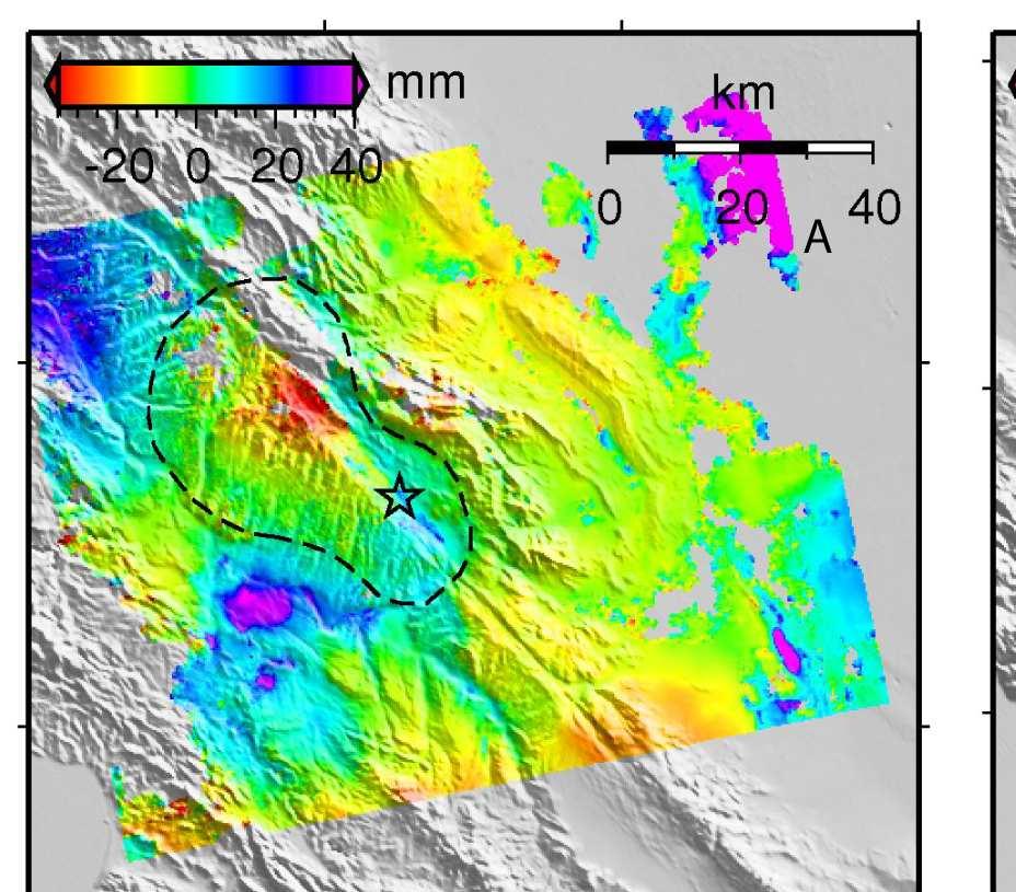
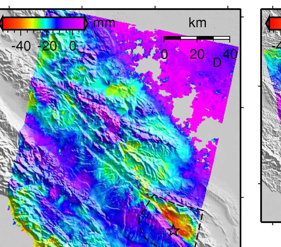
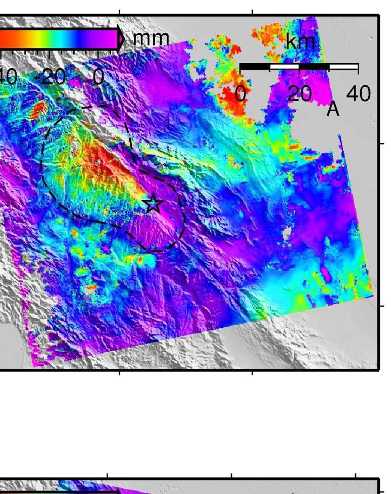
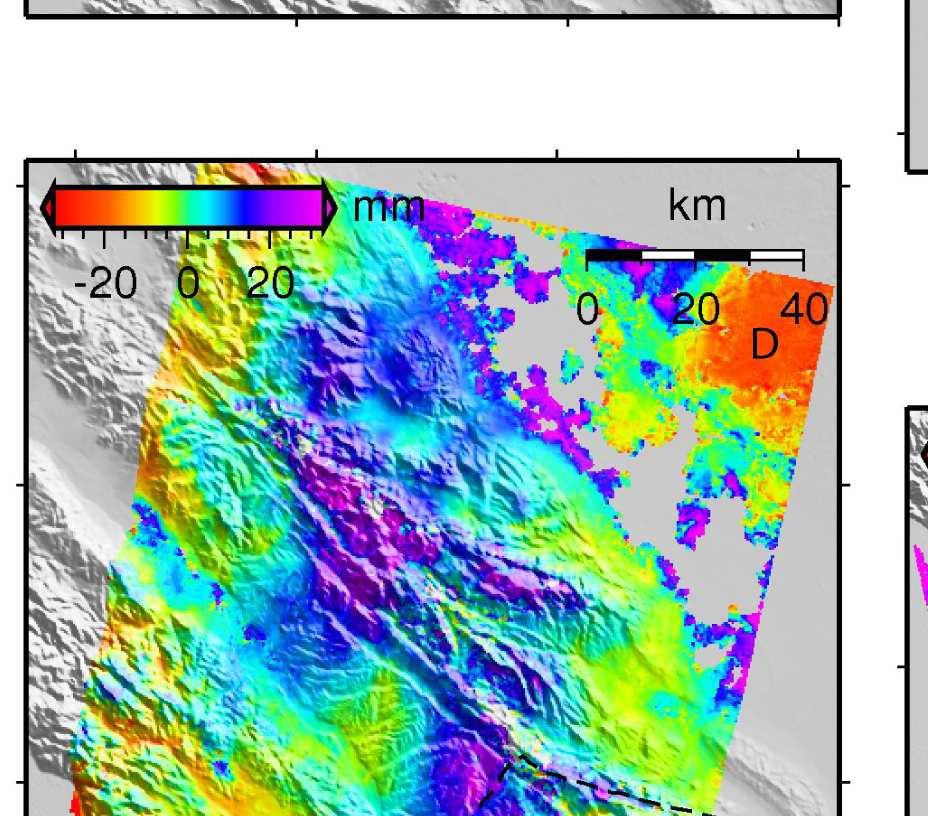
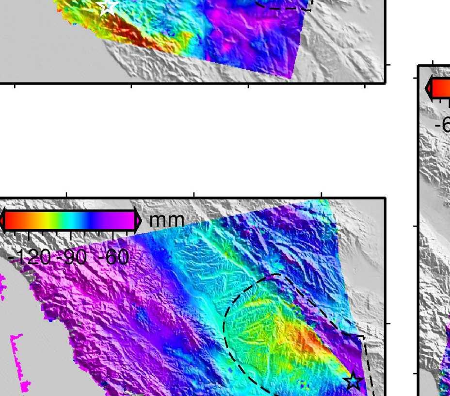
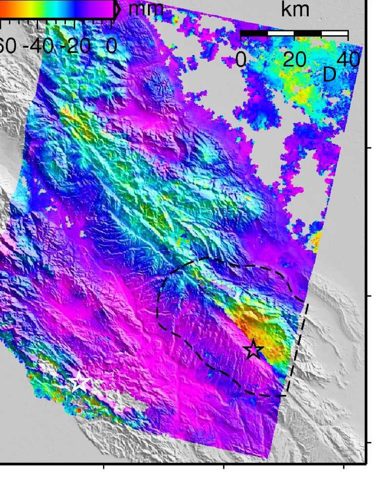
38 Figure 3.1. ENVISAT interferograms a) 3/7/2003-9/30/2004 b) 4/14/ /6/2004 c) 5/19/ /6/2004 d) 9/14/ /23/2004 e) 8/28/ /9/2004 f) 6/23/ /15/2004 Black dashed lines indicate cropped area included in model inversions. White dashed circles refer to atmospheric features mentioned in the text. Solid white circle indicated the Paso Robles subunit of the Salinas basin. Solid black circles indicate the Lost Hills oil field. Arrows are the radar look direction, with A and D referring to ascending and descending tracks respectively. The black star in all frames is the epicenter of the 2004 Parkfield earthquake and the white star is the epicenter of the San Simeon earthquake. Atmospheric Delay Nearly all interferograms suffer from contamination of the desired signal with atmospheric delay errors [Zebker et al., 1997]. Atmospheric delay errors occur when water in the troposphere slows down the travel time of the radar wave in one of the two scenes in the interferometric pair, causing an apparent change in distance. These errors are generally identifiable as long wavelength patterns or blobs of range change. In this case, areas with atmospheric delay errors can be avoided because the location and basic pattern of the target signal is known. We also expect San Andreas-fault related deformation signal to have an association with the mapped surface trace of the fault. Interferogram E shows two patches of range change to the east and southeast of Parkfield that are not near the San Andreas fault nor any other discernible tectonic structure and we interpret them to be atmospheric delay error (dashed circles in Figure 3.1e). Also, in interferograms B, C and F patches of range change to the northwest of Parkfield, in the creeping section of the San Andreas Fault, are interpreted to be atmospheric delay errors (dashed circles in Figure 3.1b, c & f). Groundwater-Induced vertical motion For the purposes of studying earthquakes or other tectonic processes, groundwaterinduced vertical motion is also a source of noise. Subsidence or rebound due to 24
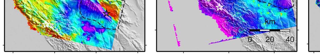
 6/19/2004-10/17/2004 b) 6/19/2004-12/28/2004 Black dashed lines indicate cropped area included in model inversions. Solid white circle indicated the Paso Robles subunit of the Salinas basin.")
39 Figure 3.2. Portions of Radarsat interferograms from ascending swaths covering the Parkfield area. a) 6/19/ /17/2004 b) 6/19/ /28/2004 Black dashed lines indicate cropped area included in model inversions. Solid white circle indicated the Paso Robles subunit of the Salinas basin. Arrows are the radar look direction, with A referring to the ascending track direction. The black star in both frames is the epicenter of the 2004 Parkfield earthquake and the white star is the epicenter of the San Simeon earthquake. variations in groundwater levels occur in many areas, and can have seasonal cycles and long-term components [Amelung et al., 1999; Schmidt and Bürgmann, 2003]. All of the interferograms contain the southern portion of the Salinas Basin including the Paso Robles subunit, just southwest of Parkfield (white circles in Figure 3.1a and Figure 3.2a). In 1997, a seasonal change in groundwater levels of 60 feet in the Paso Robles subunit, produced 6 cm of vertical ground motion or two fringes in an interferogram [Valentine et al., 2001]; an amount that is similar to the range change produced by the Parkfield earthquake. Small bulls-eye shaped range-change patterns in the Paso Robles subunit, just southwest of Parkfield, are apparent in all the interferograms, but are most obvious in interferogram A (Figure 3.1a). Interferogram A also exhibits an area of range change increase to the northwest that we interpret to be due to subsidence of the greater Salinas basin. Petroleum and gas withdrawal from shallow reservoirs can also cause rapid ground 25
40 subsidence, including at the Lost Hills oil field at the southeast corner of Interferograms A and E (black circles in Figure 3.1a & e) [Fielding et al., 1998]. This intense deformation is far enough away from the Parkfield earthquake that it is outside the area used in our analysis. The 12/22/2003 San Simeon earthquake The Parkfield earthquake occurred less than a year after the M w 6.5 San Simeon earthquake and about 50 km to the west. Southern California Integrated GPS Network (SCIGN) continuous GPS stations in the Parkfield area show coseismic motion in a westward direction of up to 1 cm from this event [Ji et al., 2004; Rolandone et al., Submitted] (Table B.2). Postseismic deformation following the San Simeon earthquake is indicated by transient motions of six GPS stations in the region, which rapidly decayed in the aftermath of the event Savage et al. [2005]; Rolandone et al. [Submitted]. Rolandone et al. [Submitted] find that the motions are best explained by afterslip in the upper 3 km of the crust. The continuous GPS sites in the Parkfield area do not reveal significant San Simeon postseismic motion. Interferogram A (Table 3.2) is the only interferogram used that also spans the San Simeon event. Estimates for the coseismic displacements from a model of GPS and InSAR data spanning the San Simeon earthquake (Section 4.4) were removed from this interferogram. Though the amount of displacement in the Parkfield area from the San Simeon earthquake was significant, the displacement gradient was small and nearly constant. Similarly, the San Simeon postseismic deformation pattern at Parkfield is very small and long-wavelength compared with the deformation signal from the Parkfield earthquake. Any remaining residual far-field displacement gradients from the San Simeon event can be compensated for by including a ramp across the interferograms as part of the model parameters (see Section 3.3.5). 26
41 Interseismic Deformation The interferograms used here have variable time-spans and each contains a different contribution from the interseismic deformation field. In the Parkfield area, the interseismic deformation field is the result of the combination of strain accumulation on the regional fault system and steady fault creep. The deformation field from strain accumulation is generally modeled as slip on large dislocations below the seismogenic portion of the fault (e.g. from km depth) and produces a deformation pattern with wavelength of tens to hundreds of km. Interseismic creep, on the other hand, involves slip on the shallow portions of the fault zone and so produces a shorter wavelength deformation pattern. The Parkfield segment of the San Andreas fault exhibits interseismic creep and is also accumulating strain energy to be released in earthquakes. To forward predict and remove the interseismic displacement field from each interferogram and to predict the interseismic velocity of the campaign GPS stations, we use an interseismic slip model from Rolandone et al. [2004]. Their model is derived from an inversion of continuous and campaign GPS data along the creeping section of the San Andreas fault and the northern and southern transition zone. It contains both deep and shallow model fault elements to capture the effects of strain accumulation and aseismic creep. Unwrapping Errors Standard algorithms for unwrapping of the interferogram phase assume that the phase varies smoothly. A discontinuity in the deformation pattern and phase, such as at a surface rupture, requires the unwrapping algorithm to estimate by how many multiples of 2π the phase of the two sides are separated. This is no problem where interferograms are continuous and unwrapping is possible around the tips of the rupture. To facilitate unwrapping under less ideal conditions, it is sometimes necessary 27
42 to subtract an a priori model of the deformation during the time spanned by the interferogram. Subtracting the phase predicted by a model reduces the phase gradients and insures that the two sides of the fault are offset by the correct multiple of 2π. We applied such a model to aid the unwrapping of interferograms D, E and F (Table 3.2). Displacements were estimated for SCIGN network continuous GPS sites for times matching the time-spans of the interferograms and include coseismic and postseismic motions. The estimated displacements were inverted for right-lateral strike-slip on a distributed slip model with geometry identical to that described below for the joint inversion. Predicted range changes from the model for each interferogram were subtracted before unwrapping and added back in afterwards. Including these models facilitated successful unwrapping across the SAF zone, however the Parkfield earthquake involved surface slip on two sub-parallel strands 2 km apart. The Southwest Fracture Zone (SWFZ) slipped coseismically at the surface, while the main trace of the SAF exhibited enhanced postseismic creep [Langbein et al., 2005; Langbein and Murray, Submitted]. The GPS data used to create the a priori model are not dense enough to constrain slip on both strands, so our model includes only a single fault plane at depth and at the surface. The unwrapping algorithm must decide how to partition the phase change across both strands using information from more smoothly varying parts of the interferogram. This makes the area between the two strands particularly susceptible to unwrapping errors Global Positioning System (GPS) We use GPS-derived horizontal displacements from both campaign and continuous stations (Figure 3.3, Table B.2). The campaign data includes five stations surveyed by UC Berkeley and 12 stations surveyed by the USGS. The campaign data were processed in daily solutions using GAMIT and combined, using GLOBK/GLORG, 28

43 Figure 3.3. Locations of GPS stations used in this study. Triangles are stations in the SCIGN continuous GPS network, diamonds are recently added PBO continuous stations, squares are campaign stations surveyed by the USGS and inverted triangles are campaign stations surveyed by UC Berkeley. Dashed line is spatial extent of Figure 3.4. Reference stations ORES is shown in inset map. with daily solutions from continuous stations in the SCIGN network and the International GNSS Service (IGS), obtained from the Scripps Orbital and Permanent Array Center [ Continuous sites from the Earthscope/PBO network that were installed within a month after the Parkfield earthquake are also included to constrain the postseismic slip. Time-Series Modeling We used time-series modeling to extract the coseismic and postseismic displacements at each GPS station and used these as inputs in the simultaneous slip inversion. The SCIGN continuous GPS stations provided the most complete record of station 29
44 displacements and were fit by the model given below. d total = c + v int t + d ss H (t t ss ) + d pk H (t t pk ) d ps (1 exp ( (t t pk ) /τ))h (t t pk ) (3.1) Where H(t) denotes the heavyside step function. A constant (c), the interseismic velocity (v int ), offsets at the times of the San Simeon (d ss ) and Parkfield (d pk ) earthquakes and the amplitude (d ps ) and decay time (τ) of the exponential were solved for using a simplex search method for unconstrained nonlinear optimization to minimize the residual sum of squares. The results of the time-series modeling are shown in Table B.2 in Appendix B. Campaign GPS Time-Series Modeling The time-sampling of the campaign stations and the Earthscope/PBO stations is more sparse than the SCIGN stations. For these sites, subsets of the model parameters in Equation 3.1 were solved for. The specific subset was chosen for each data source (UCB, USGS or Earthquake/PBO) according to the specific times of observations. For all three of the data sources listed, the interseismic slip model described in Section was used to constrain the interseismic velocities. The five UC Berkeley campaign stations were surveyed three times before the Parkfield earthquake. Though they were displaced by the San Simeon earthquake in 2003, two surveys were conducted between the times of the San Simeon and Parkfield earthquakes. The offsets from both earthquakes can therefore be solved for despite the sparse time sampling of the observations. However, we are not able to determine either the amplitude of the postseismic exponential decay or the decay time constant from the UCB campaign GPS data. Campaign stations surveyed by the USGS did not include observations between 30
45 the times of the San Simeon and Parkfield earthquakes. In this case, we cannot uniquely determine offsets due to each event. However, many of the stations were surveyed quasi-continuously after the Parkfield earthquake and we were able to solve for the amplitude of the postseismic exponential given an imposed decay time constant (0.14 years). The Earthscope/PBO continuous stations installed after the Parkfield earthquake were treated like campaign data in that a priori interseismic velocities were used, the postseismic amplitude was solved for, and the decay time constant was fixed to 0.14 years. It was possible to solve for a coseismic offset for four Earthscope/PBO stations installed before the Parkfield earthquake. However, these four sites were located distant from the Parkfield rupture area, and the amplitude of the postseismic displacement was too small to be determined 3.3 Simultaneous Coseismic and Postseismic Slip Inversion Earthquake cycle effects All of the datasets used here contain contributions from the coseismic, postseismic and interseismic periods of the earthquake cycle. The different time spans and sampling of the datasets mean that they contain different ratios of coseismic, postseismic and interseismic deformation. This fact is used to our advantage in the model presented here in order to differentiate between coseismic and postseismic slip. The postseismic slip is assumed to evolve with the same exponential decay function as the GPS sites (Equation 3.1), such that the total slip (s total ) has the following form, s total = s cs + A ps ( 1 e t ps/τ ) (3.2) 31
46 where t ps is the amount of postseismic time spanned by each interferogram or GPS dataset; that is, the amount of time between the Parkfield earthquake and the end of the dataset. Daily time series from continuous GPS stations and USGS creepmeter data were used to constrain the decay time constant (τ) and thereby predict the fraction of the total postseismic deformation field included in each dataset (Section 3.3.4). A joint inversion was then performed on the InSAR and GPS data for the coseismic slip (s cs ) and exponential decay amplitude (A ps ) on each model element. It should be noted that by solving for only A ps, we do not allow the spatial distribution of postseismic slip to change over time. Nonetheless, this approach allows us to take advantage of the number of interferograms available to constrain the model while accounting for the variable time span of each Data Reduction Because the desired signal in the interferograms is of similar magnitude to the noise sources, as discussed above, it became necessary to crop the interferograms to include only the Parkfield region (dashed lines in Figure 3.1 & Figure 3.2). In addition to not considering areas well outside of the coseismic deformation zone, the cropped regions were chosen to avoid known areas of petroleum withdrawal and groundwater-induced vertical motion, such as the Paso Robles subunit, and those areas determined to be heavily contaminated by atmospheric errors. The areas inside the cropped region are not necessarily free of noise sources, but they have a signal to noise ratio high enough that the range change related to the Parkfield earthquake will dominate the inversion. The interferograms were further sub-sampled on a grid with 1 km spacing, where each sample is an average of 16 pixels. This mitigates any correlations that exist between pixels, particularly those introduced by filtering. 32

47 3.3.3 Model Geometry With interseismic deformation removed, we can restrict our inversion to a single, vertical, 40 km x 15 km plane, which is divided into km x 1 km elements. The 2004 Parkfield earthquake involved slip on multiple surface traces of the SAF as described in Section Although the interferograms include range change estimates across the entire rupture zone, there is a possibility of unwrapping errors in this area. We therefore choose not to model the complex surface rupture pattern, but instead focus on the slip at depth. Our model plane was chosen to strike midway between the SAF main trace and the SWFZ (Figure 3.4). The interferogram samples Figure 3.4. Locations of continuous SCIGN GPS stations (squares) and creepmeters (circles) used to contstrain the decay time constant. Bold black line is the surface projection of the model fault plane. Reference stations ORES is shown in inset map. located between the main trace and the SWFZ, and continuous GPS station CARH, were removed from the inversion. An offset between the model plane and the actual surface rupture will tend to cause surface slip to be mapped onto deeper model fault elements. However, the SAF 33
48 and the SWFZ are within 1-2 km of our model plane, so this effect is expected to be minimal and to be restricted to the top 1-2 km depth. The shallow elements in our model reflect the sum of shallow slip across the active strands Postseismic Exponential Decay Time Constant We use data from 12 continuous GPS stations and six USGS creepmeters to constrain the postseismic exponential decay time constant (τ). We applied the model of Equation 1 to records of daily displacement from creepmeters XMM1, XMD1, XVA1, WKR1, CRR1 and XGH1 (Figure 3.4 and Table B.3). We used the values determined for the north and east components of SCIGN stations CAND, CARH, HOGS, HUNT, LAND, MASW, MIDA, MNMC, TBLP and RNCH and the east components of stations PKDB and POMM (Figure 3.4 and Table B.2). Figure 3.5 shows the values of the decay time constant as a function of the perpendicular distance from the San Andreas Fault. The lack of a systematic trend in these values indicates that postseismic slip from deep and shallow depths on the fault did not occur with significantly different decay times. Particularly the fact that the creepmeter estimates are similar to the GPS estimates from further away from the fault indicates that surface creep did not evolve differently than slip at depth. The decay time constant used in the inversion (0.17 years) is the median of the decay time constants determined from the creepmeter records and the selected continuous GPS time-series. 34
49 Figure 3.5. Decay time constants fit to continuous GPS and creepmeter data. Dashed line shows value (0.17 years) used in the model. Uncertainties for the creepmeter data average years; error bars would be about the size of the symbol Inversion set-up We invert the eight interferograms and four GPS datasets simultaneously for the coseismic slip and the amplitude of the postseismic exponential decay as follows, 1 αg s1 αg s1 (1 exp ( (t ps1 t pk ) /τ)) xy 1 α d s1.... αg sn αg sn (1 exp ( (t ps1 t pk ) /τ)) xy N α s cs d sn W gc G gc 0 0 = Aps W gc d gc 0 W gp G gp 0 t W gp d gp β 2 β (3.3) where d s is the vector of InSAR samples. s cs is the vector of coseismic offsets and Aps is the vector of amplitudes of the postseismic decay, taken directly from Equation 3.1. G s1 N, G gc and G gp are Green s functions for the InSAR, coseismic GPS 35
50 and postseismic GPS data respectively. The Green s functions are constructed using Okada s equations [Okada, 1985] to relate unit slip on each dislocation to displacements at the surface. t ps1 N are the ending times of the interferograms (Table 3.2) and t pk is the time of the Parkfield earthquake. The InSAR data is weighted in the inversion relative to the GPS through the factor α, which is chosen so that the InSAR data has twice the weight of the GPS data. The choice to weight the InSAR data more heavily was made because of the greater quantity of InSAR data. The Laplacian operator ( 2 ) was used to apply smoothing to the modeled slip and is weighted by β. It is constructed to smooth the model towards zero slip at the northwest, southeast, and bottom edges of the model plane. We further constrain the model to allow only right-lateral strike-slip by implementing a bounded-value least-square algorithm to perform the inversion [Stark and Parker, 1995]. xy N are the Green s functions relating the interferogram samples to an offset and gradient across the interferogram ( t ). A gradient is typically included in inversions of InSAR data to account for possible errors in the orbit parameters. However, since the interferograms have been cropped to a fraction of the size of the original radar scene, a scene-wide gradient from orbit parameter errors would be very small within the cropped region. Solving for a ramp on the small subset could imply a large phase error in the distant parts of the interferograms that is unrealistic. We nonetheless include the ramp terms in the inversion to also account for noise sources, such as atmospheric water vapor variations, with a wavelength greater than the cropped region that might appear ramp-like across the samples. For example, in the cropped areas of the interferograms, postseismic displacements from the San Simeon earthquake are nearly a ramp and can be compensated for with this additional model term. 36
51 3.4 Results and Discussion Figure 3.6 shows the results of the inversion for coseismic slip and for the total slip amplitude ( A ps ) of the postseismic exponential. The model fits to the data are Figure 3.6. Results of inversion for a) Coseismic slip b) Amplitude of postseismic exponential. Red stars mark location of earthquake hypocenter. Gray circles are double-difference relocated aftershocks [Thurber et al., Submitted], size of circle is size of rupture assuming 3 MPa stress drop and circular rupture. Letters A, B & C refer to asperities mentioned in the text. Triangles are color-coded creepmeter displacements with time spans described in the text. shown in Figure 3.7 and Figure 3.8. The coseismic slip occurred in two asperities: 37
52 Figure 3.7. Model fits to InSAR data. Letters refer to interferograms listed in Table 3.2. LV: Look vector, direction of satellite view. 38
53 Figure 3.8. Model fits and residuals for the GPS data. Top row is stations with coseismic estimates (d gc in Equation 3.3) and their fit to the coseismic slip model. The bottom is stations with postseismic amplitudes (d gp in Equation 3.3) and their fit to the postseismic slip model. Displacements are relative to station ORES (Figure 3.3). 95% confidence error ellipses are plotted with the observations. 39
54 Asperity A is located near the hypocenter and Asperity B is km northwest of the hypocenter. The postseismic slip has a maximum north of Asperity B and deeper on the fault surface (Asperity C), near two M w 5.0 aftershocks. Much of the rest of the postseismic slip occurs in the shallow portions of the fault. In the northwestern half of the model, the coseismic and postseismic slip patterns appear complementary to each other. Asperity B is an area of high slip in the coseismic model, but the same area experiences little postseismic slip. Similarly, Asperity C is located in an area in which no slip was resolved in the coseismic model. The regions of enhanced postseismic slip occur near the edges of the coseismic slip, in areas that would have experienced increased stress from the coseismic rupture. This is consistent with the view that velocity-strengthening segments of the San Andreas fault experienced transient accelerated slip in response to the Parkfield stick slip event. Johnson et al. [Submitted] developed a rate-state friction model of afterslip constrained by the postseismic continuous GPS time-series. The inversion was repeated using only the InSAR data and then only the GPS data and the results are shown in Figure 3.9. The separate inversions have limited Figure 3.9. Comparison of inversion using only InSAR data (left) and only GPS data (right). Annotations are same as for those in Figure
55 resolution power along different portions of the model where either GPS stations or coherent InSAR data are sparse. In the coseismic model, the pattern of slip in both single-datatype inversions is similar and suggests that the results found here are not overly sensitive to dataset weighting (α). However, for the postseismic slip models, the GPS data prefer more shallow slip than the InSAR data. Though both inversions resolve enhanced postseismic slip north of SAFOD, the inferred slip occurs at different depths; the GPS only inversion favors surface slip here, while the InSAR and the joint inversions do not. Figure 3.10 shows the results of reducing the smoothing weight by half and of doubling it. The main features of the coseismic slip pattern (the double Figure Comparison of inversion where smoothing factor has been reduced by half (left) and doubled (right). Annotations are same as for those in Figure 3.6. asperity) are not changed in either result. The postseismic slip model appears to be quite sensitive to the smoothing factor. Several slip patches in the low smoothing models disappear in the high smoothing model and north of SAFOD the location of slip changes from near surface to below the surface. This change in depth of the northern slip patch as the smoothing is increased is similar to the difference between the GPS to InSAR only models. This indicates that as the smoothing is increased, the InSAR is favored more. This is probably because the GPS data are concentrated near 41
56 the fault s surface trace, whereas the InSAR samples are more broadly distributed. As the smoothing smears out the slip asperities, deeper parts of the fault, which are most sensitive to the InSAR data, are required to slip Relationship to aftershocks The coseismic model is plotted with aftershocks that occurred on September 28 from a catalog of double-difference relocated events [Thurber et al., Submitted]. The postseismic slip model is plotted with relocated aftershocks from Sep. 29 through Nov. 17. Langbein et al. [2005] note that the relocated aftershocks occur in the same clusters and streaks as the pre-earthquake background seismicity, including a streak which is visible in the aftershocks at about 5 km depth. One interpretation of microseismicity streaks is that they occur at the boundaries of creeping and locked asperities of the fault surface [Nadeau et al., 1995]. Thus, the streak of aftershocks at 5 km depth occurs near the top of Asperity B, and could be interpreted as weakly bounding the asperity. Furthermore, a smaller streak of aftershocks near the hypocenter at 9 km depth lies near the top of Asperity A. In the postseismic slip model, much of the shallow slip occurs in the fault region above the 5 km aftershock streak. That the streak forms a sort of dividing line between coseismic and postseismic slip suggests that it does indeed occur at the boundary of velocity-weakening and velocity-strengthening fault zone materials. The area of enhanced postseismic slip to the northwest corresponds with the location of two M w 5.0 aftershocks that occurred on September 29 and 30. Assuming a 3 MPa stress drop and circular rupture, these events contributed 13 cm of slip to the postseismic slip model. However, the model indicates as much as 26 cm of slip over a similar area and suggesting that aseismic slip of as much as 13 cm occurred near the aftershock hypocenters. Our model cannot address the relative timing of the 42
57 aftershocks and the surrounding aseismic slip and whether the earthquakes occurred in response to increased creep rates or if they unpinned the fault surface and allowed enhanced creep to take place Surface Slip Creepmeter displacements for instruments on the SAF main trace are also plotted in Figure 3.6 for comparison. Negligible creep was recorded on SWFZ creepmeters XHSW and XRSW. Several of the USGS creepmeters went off-scale during or just after the Parkfield earthquake and had to be reset by hand. The total fault displacement while the instrument was off-scale was measured with a micrometer. We plot the displacements from before the earthquake to after the instrument was brought back on-scale with the coseismic slip model. Displacements from when the instruments were reset to Jan. 31, 2005 are plotted with the postseismic slip model. Early postseismic slip occurred rapidly in some areas, so we expect the coseismic creepmeter displacements to be an overestimate and the postseismic displacements to be an underestimate. Nonetheless, our model correctly captures the overall magnitude and some of the features of the surface slip distribution. According to the coseismic model, surface slip continued at low levels north of Middle Mountain up to near the San Andreas Fault Observatory at Depth (SAFOD). Surface slip in the coseismic model terminates at Gold Hill in the south (creepmeter XGH1), although postseismic surface slip continued for another 6 km. This extent of surface slip in the models is similar to field observations, where patches of ground breakage were observed just south of SAFOD and extended south until about 10 km south of Gold Hill [Langbein et al., 2005]. 43
58 3.4.3 Seismic vs. Aseismic Moment Release The model yields a moment estimate of Nm (M w 6.2) for the coseismic period and Nm (M w 6.1) for the postseismic period. Because the postseismic slip model is derived from the amplitudes of the postseimic exponential decay, the postseismic moment magnitude is not associated with any particular time-span, but is an estimate of for the entire postseismic period. The total moment for both periods is Nm (M w 6.3). The coseismic moment magnitude is larger than the seismic estimate of M w 6.0 [Dreger et al., 2005]. This could partly be due to aseismic slip from early in the postseismic period being included in our coseismic model. If the coseismic moment magnitude was M w 6.0, as much as 70% of the slip in our 1- day model is aseismic; 55% if the seismic moment magnitude were M w 6.1. That the Parkfield earthquake produced rapid postseismic slip with moment nearly equal to the coseismic rupture could be related to the Parkfield earthquake s delay from the original prediction and the extra moment deficit that was allowed to accumulate. Rapid and copious postseismic slip was also observed following the 1966 Parkfield event [Smith and Wyss, 1968] and for several subduction zone earthquakes [Bürgmann et al., 2001; Heki et al., 1997]. The profusion of postseismic, aseismic slip at these locations is almost certainly related to their transitional nature (including both locked and creeping fault areas) and the juxtaposition of velocity-strengthening and velocityweakening fault materials. In fact, geodetic estimates of combined coseismic and early postseismic moment release for the 1934 and 1966 Parkfield earthquake have consistently obtained estimates in the range of M w [Murray and Segall, 2002; Segall and Du, 1993; Segall and Harris, 1987; Murray and Langbein, Submitted]. The similarity of our observations and results for the 2004 Parkfield earthquake to those for the earlier events is evidence that these events are to some extent characteristic earthquakes. Segall and 44
59 Du [1993] also obtained an estimate for the geodetic moment magnitude of M w 6.4 for the 1934 Parkfield earthquake. Large amounts of postseismic slip appear to be characteristic of the Parkfield area and underscore the need to explicitly consider aseismic slip in any time-predictable model of earthquake occurrence in transition zones. 3.5 Conclusions We simultaneously inverted InSAR and GPS data for coseismic (event plus 1-day afterslip) and postseismic slip from the 2004 Parkfield earthquake. The model indicates that coseismic slip occurred as two asperities, with the larger being northwest of the hypocenter by 15 km. For the postseismic period, the model identifies a deep slip asperity near the location of two M w 5.0 aftershocks. The slip model suggests that a streak of microseismicity at 5 km depth forms a dividing line between coseismic slip below and postseismic slip above. In general, postseismic slip is enhanced in the areas directly surrounding the coseismic rupture and most shallow slip occurred during the postseismic period. The model indicates that the rupture extended from 6 km south of Gold Hill to near SAFOD. We obtain an estimate of the moment magnitude of M w 6.2 for the slip during 1 day including the coseismic rupture and M w 6.1 for the subsequent postseismic period. The difference between our coseismic estimate and the seismic moment magnitude of M w 6.0 implies that our model contains substantial early afterslip and that as much as 70% of the of the total moment release associated with the Parkfield earthquake occurred aseismically. 45
60 Chapter 4 Influence of stress change from the 2003 San Simeon earthquake on rupture during the 2004 Parkfield earthquake 4.1 Introduction The 2004 Parkfield earthquake was the long-awaited fulfillment of the Parkfield Earthquake Prediction Experiment. A series of M 6 earthquakes with a recurrence interval of 22 years, prompted Bakun and Lindh [1985] to predict that the next M6 earthquake would occur in The Parkfield segment became one of the best-instrumented fault segments in the United States and though the predicted earthquake occurred 16 years late, it promises to provide valuable insight into earthquake processes. Not only did the past Parkfield earthquakes occur with quasi-regularity, but their 46
 and propagated to the southeast along the San Andreas fault [Bakun and McEvilly, 1979, 1984]. Triangulation and trilateration Figure 4.1. Locations of GPS stations used in this study.")
61 rupture patterns also shared several characteristics. Analysis of the seismograms from the 1922, 1934 and 1966 earthquakes indicate that they all had hypocenters near Middle Mountain (Figure 4.1) and propagated to the southeast along the San Andreas fault [Bakun and McEvilly, 1979, 1984]. Triangulation and trilateration Figure 4.1. Locations of GPS stations used in this study. Triangles are continuous stations, squares are campaign stations. Grey stars are epicenters of 1934, 1966 and 2004 Parkfield earthquakes. Black star is epicenter of the San Simeon earthquake. Dashed line shows outline of InSAR scene. surveys before and after the 1934 and 1966 earthquakes also indicate that the peak slip in all the prior events occurred 10 km south of their hypocenters [Segall and Du, 1993; Murray and Langbein, Submitted]. The Parkfield Prediction Experiment was thereby a test of the characteristic earthquake model, as well as a test of the timepredictable model. The 2004 Parkfield earthquake was similar to the past events in that the coseismic rupture had a moment magnitude near M6.0 and peak slip 10 km south of Middle Mountain [Johanson et al., Submitted; Murray and Langbein, 47
62 Submitted]. However, it differed from the characteristic pattern established by the Parkfield earthquakes since its hypocenter was located south of Parkfield and rupture propagated northwest [Langbein et al., 2005] The Parkfield Earthquake s Delay Several hypotheses exist for why the Parkfield earthquake was delayed by 16 years relative to the original prediction. Ben-Zion et al. [1993] proposed that interactions between segments of the San Andreas fault and viscous relaxation of the lower crust and upper mantle since the 1857 Fort Tejon earthquake, modulate the loading rate on the Parkfield segment. The decay in the recurrence rate of the Parkfield earthquakes could then be due to the decaying effect of the Fort Tejon earthquake. In their modeling, the predicted date of the next Parkfield earthquake depended on the chosen viscosity parameters; however, estimates used in the study suggested the effect was to delay the occurrence of the Parkfield earthquake to ± 9-11 years. A multi-year fault slip transient was detected by borehole strainmeters [Gwyther et al., 1996], repeating earthquake frequency changes [Nadeau and McEvilly, 1999] and continuous GPS and EDM data [Murray and Segall, 2005]. It occurred from , a time period that saw an increase in the amount of microseismicity and four earthquakes with magnitudes 4.2, 4.6, 4.7 and 5.0 [Nadeau and McEvilly, 1999]. The transient slip event involved accelerated shallow slip (creep) near the hypocenters of the previous Parkfield earthquakes. It had an equivalent moment magnitude of M and reduced the total slip deficit on the Parkfield segment [Langbein et al., 1999; Gao et al., 2000; Murray and Segall, 2005]. Under a time-predictable earthquake reccurrence model this would translate into a delay of the characteristic earthquake s occurrence. Moreover, the transient slip event and/or the accompanying earthquakes 48
63 may have released stress near the hypocenter (nucleation site) of the 1966 and 1934 Parkfield earthquakes [Murray and Segall, 2005]. Stress changes from the 1983 Coalinga-Nuñez thrust mechanism earthquakes also affected the Parkfield segment and decreased microseismicity rates along portions of the San Andreas fault. The areas of decreased microseismicity corresponded to areas where shear stress had been decreased and likewise areas where shear stresses were increased by 0.5 bars corresponded to increased micro-seismicity rates [Toda and Stein, 2002]. Toda and Stein [2002] calculated that the probability of a M 6 earthquake at Parkfield decreased by about 12% immediately after the Coalinga event, based on a decrease in the coulomb failure stress near the 1966 hypocenter (Figure 4.1). However, they also calculate, using rate-and-state friction formulations, that the influence of the Coalinga-derived stress changes decayed over the next eight years and that the probabilities returned to their unperturbed values by If the Parkfield segment is sensitive enough to stress perturbations to be delayed by these previous events, then its occurrence nine months after the San Simeon earthquake could be more than coincidence. Preliminary estimates suggest Coulomb stress increased on the Parkfield segment by nearly 0.3 bars [Langbein et al., 2005]. Though small, stress changes of as little as 0.1 bars have been observed to correlate with the locations of aftershocks [Stein, 1999; Harris, 1998], and future main shock hypocenters [e.g. Parsons and Dreger, 2000; Stein et al., 1997]. Here, we use space geodetic data to develop a slip model for the 2003 San Simeon earthquake (SSEQ). We calculate the static stress changes along the San Andreas fault produced in both the coseismic and postseismic periods of the SSEQ and investigate whether they promoted the 2004 Parkfield earthquake (PKEQ), influenced the slip distribution and/or contributed to the change in hypocenter location from that of the previous Parkfield earthquakes. 49
64 4.1.2 The Role of the 12/22/2003 San Simeon Earthquake The 9/28/2004 Parkfield earthquake occurred less than a year after the M6.5 San Simeon earthquake of 12/22/2003. The San Simeon earthquake was a thrust event in the Central California Coast Range ( 50 km west of the Parkfield segment), which accommodated shortening normal to the plate-boundary direction [Hardebeck et al., 2004]. The Berkeley Digital Seismic Network (BDSN) moment tensor solution resolves nodal planes striking 290 and 131 and dipping 58 NE and 34 SW respectively. Finite fault inversions show a slight preference for the steeply northeast-dipping plane [Ji et al., 2004; Rolandone et al., Submitted]. The northeast-dipping plane is also consistent with slip on a northeast-dipping Oceanic fault (Figure 4.1), although no surface rupture was reported to confirm this as the responsible structure [Hardebeck et al., 2004]. Aftershocks occurred mostly within the apparent hanging-wall block and while they tend to encircle the rupture area on the northeast dipping plane, they also appear to delineate a conjugate structure near the San Simeon epicenter [Hauksson et al., 2004]. Postseismic processes have also been implicated in earthquake triggering. Postseismic afterslip from the 1999 Izmit earthquake nearly doubled the input stress at the hypocenter of the Düzce earthquake, which occurred 87 days later [Hearn et al., 2002]. Postseismic stress changes may also influence the rupture pattern of future earthquakes. Stress changes from postseismic relaxation following the 1992 Landers earthquake show a better correlation with the Hector Mine rupture area than those from coseismic slip [Freed and Jin, 2001]. The effect of stress changes from postseismic afterslip or viscous relaxation can also help explain the delay of months to years for some triggered earthquakes. The seven year separation between the 1992 Landers and the 1999 Hector Mine earthquakes has been explained both as the result 50
65 of rate-and-state friction [Price and Bürgmann, 2002] and as the effect of postseismic processes [Freed and Jin, 2001; Pollitz and Sacks, 2002]. For the Landers and Hector Mine earthquake pair, Harris and Simpson [2002] found that small changes in the Landers coseismic slip model affected whether stresses at the hypocenter of the Hector Mine earthquake were calculated to have increased or decreased. We therefore begin by performing a search for the optimal orientation of the rupture plane, as required by the data. Then several rupture scenarios for the SSEQ are explored, including slip on a bent plane, allowing a variable rake angle, and allowing for postseismic afterslip. We use our preferred slip models from this analysis to examine the static stress change fields and their impact on SSEQ aftershock occurrence and on the Parkfield segment. 4.2 Data InSAR We use SAR data from beam 2 of the European Space Agency s Envisat satellite. Interferograms are formed from the difference in phase of a scattered radar pulse from satellite acquisitions on two separate occasions. The phase difference is proportional to the change in distance between the ground and the satellite between the two acquisition dates (range change) and thus provides a measure of ground deformation [see Bürgmann et al., 2000, for more detail]. Envisat made only one pre-earthquake acquisition over the San Simeon rupture area on 12/9/2003, only 13 days before the San Simeon earthquake. For the purposes of detecting ground deformation, the orbit paths of the two satellite fly-bys should be as close as possible. If the distance between the orbit paths (specifically the perpen- 51
![dicular baseline) exceeds a certain value, which depends on the scattering properties of the ground cover, the interferogram will consist of random noise (decorrelation) [Bürgmann et al., 2000].](/docs-images/86/94575211/images/66-0.jpg "While there are several post-earthquake acquisitions, including ones on 6/1/2004, 7/6/2004 and 8/10/2004, it is not until the acquisition on 9/14/2004 that the perpendicular baseline between the")
66 dicular baseline) exceeds a certain value, which depends on the scattering properties of the ground cover, the interferogram will consist of random noise (decorrelation) [Bürgmann et al., 2000]. While there are several post-earthquake acquisitions, including ones on 6/1/2004, 7/6/2004 and 8/10/2004, it is not until the acquisition on 9/14/2004 that the perpendicular baseline between the preseismic and postseismic satellite orbits is short enough to make a useful interferogram (Figure 4.2). The Figure 4.2. Wrapped interferogram spanning from 12/9/2003 to 9/14/2004. Black star is San Simeon EQ epicenter. Black arrow indicates orientation of converging fringes in the northwest. 9/14/2004 acquisition occurred just prior to the Parkfield earthquake of 9/28/2004, thus the interferogram contains both deformation from the San Simeon earthquake and nearly all postseismic deformation leading up to the Parkfield event. This inter- 52
67 ferogram is therefore not only well suited to investigate the slip characteristics of the San Simeon earthquake, but also any possible relationship between the San Simeon and Parkfield events. The interferogram was processed using the ROI PAC software package, and unwrapped using a branch-cut method. The interferogram was sub-sampled to reduce the number of observation points to a manageable number and to mitigate the effect of correlated errors between nearby pixels either inherent to the interferogram or introduced by filtering. The interferogram was sub-sampled with three grid spacings (Figure 4.3). Within a km box around the approximate center of the rup- Figure 4.3. Data used in this study, including InSAR samples given in mm of range change and GPS displacements. ture, the sample spacing is 1 km. Outside of this box and within a km area, the sample spacing is 2 km. Elsewhere in the interferogram, the sample spacing is 5 km. The three tiers of sample spacing have the effect of more heavily weighting 53
68 the near-field points, which contain more information about the earthquake rupture, than the far-field points Global Positioning System (GPS) We use the coseismic GPS displacements of Rolandone et al. [Submitted]. The set consists of 35 stations, including continuous stations in the SCIGN Parkfield Network, four continuous stations operated by the University of Wisconsin [Titus et al., 2005] and campaign observations by the USGS, JPL and UC Berkeley (Figure 4.1). For the continuous stations, the coseismic displacements are the difference between the average of four days before and the average of the four days after the San Simeon earthquake. For the campaign stations, the pre-earthquake position was extrapolated using an interseismic velocity. The interseismic velocities were determined either by fitting a time-series of pre-earthquake observations, or from the SCEC Crustal Motion Map [ When available, the post-earthquake positions for the campaign stations were also taken to be the average of the first four days after the earthquake. When not available, the post-event observations were corrected for postseismic motions and the post-earthquake position was estimated by extrapolating back to the time of the event using a postseismic afterslip model derived from six postseismic time series [ The uncertainties in the GPS displacements reflect both the formal errors from the position processing as well as the uncertainties in interseismic velocities or postseismic correction, when used. 54
69 4.3 Model Geometry We first solve for the best-fitting orientation of the rupture plane using a constrained non-linear search algorithm. The search algorithm adjusts the strike, dip, length, width and position of a single plane to find the geometry that minimizes the weighted residual sum of squares (WRSS) in a linear least-squares inversion for slip [Bürgmann et al., 1997]. The slip inversion is formulated as, 1 γg s xy γ d s s = W g G g 0 W g d g t (4.1) where d s is the vector of InSAR samples and d g is the vector of GPS displacements. G s and G g are Green s functions for the InSAR and GPS data respectively, calculated using Okada s equations for displacements at the surface due to slip on a buried dislocation in an elastic half space [Okada, 1985]. γ is the weighting factor between the InSAR and GPS data and was chosen such that γ d s = W g d g. The effect of γ is to scale the uncertainties in the InSAR data, which are assumed to be independent. The values used here correspond to assigning uncertainties of 6 cm to the InSAR data (two fringes), however this number is intended to also account for the larger number of data points in the InSAR dataset. The InSAR data are not internally weighted, however the GPS data are weighted by W g. W g is chosen such that W T g W g = χ 1 g, where χ g is the GPS data covariance matrix. xy are the Green s functions relating the interferogram samples to an offset and gradient across the interferogram ( t ). A gradient is generally included as a model parameter for inversions of InSAR data to compensate for possible errors in satellite orbit parameters. The misfit statistic, WRSS is given by, WRSS = n γ (d ns m ns ) 2 + k W kg (d kg m kg ) 2 (4.2) where d ns and d kg are elements of the InSAR and GPS data vectors respectively and 55
70 Table 4.1. Estimated fault geometry parameters. Dashes indicate parameter was not estimated in search process, but constrained to that of the starting geometry. M 0 calculated with rigidity of N/m 2 Model Strike Dip Rake Length Width Top, Center point M 0 Geometry (km) (km) Lat. Lon. Depth (Nm ) Starting (km) GPS-only [5] InSAR-only Joint Rake m ns and m kg are the modeled InSAR and GPS data. γ is the same as in Equation 4.1, while W kg is kth element of a vector composed of the sums of the columns of W g. The best-fitting geometry search was repeated for the InSAR and GPS data individually and also together, to investigate the consequences of using data with different time-spans. Differences between their optimal planes highlight the different sensitivities of the two datasets and the effect of shallow postseismic slip on the InSAR-derived model. We also performed a search for the best-fitting geometry allowing a variable rake angle. In each case, the starting plane was based on the northeast dipping nodal plane from the BDSN moment tensor with strike of 290 and dip of 58 and was chosen such that the plane intersected the hypocenter at latitude , longitude and 8 km depth. The results from each scenario are shown in Table Single Data-type Geometry Estimates The GPS data ( GPS-only plane) and the InSAR data ( InSAR-only plane) both prefer rupture planes with similar strike and dip (Table 4.1). Both also prefer a plane that is elongated along strike, and does not reach the surface. The InSAR data, however, prefers a plane 9.6 km wide down dip, while the search algorithm is constrained by the lower bound of 5 km for the width of the plane when the GPS data 56
71 Table 4.2. Weighted residual sum of squares and their improvement from the starting to the best-fitting fault plane geometry. Residuals listed are unscaled (see Section 4.3.2). WRSS GPS-only InSAR-only Joint Rake GPS starting ending InSAR starting ending is used. This may indicate that postseismic slip (which would be evident from the InSAR data) occurred deeper on the fault than the coseismic rupture. Overall, the geometry estimates using the individual data types seem to suggest that the InSAR and GPS data are compatible with a single model geometry despite spanning different amounts of time Joint Geometry Estimates We also performed a search for the best-fitting fault plane to both the InSAR and GPS data simultaneously. To ensure that improvements in WRSS for each datatype influenced the final geometry equally, the residuals to each datatype were weighted relative to each other. The weighting factor was chosen so that each datatype s residuals to the starting geometry were equal. This step is important when the algorithm must split the difference between fitting the GPS and the InSAR data. Figure 4.4 shows the location of the best-fitting fault plane for the joint estimation (referred to as the Joint plane). The Joint plane has the same strike as the GPSonly plane and the same dip as the InSAR-only plane. Table 4.2 lists the WRSS for the starting and ending geometries. The WRSS for the Joint geometry is only 57
72 Figure 4.4. Locations of best-fitting fault planes for joint inversion allowing dip-slip only ( Joint ) and allowing left-lateral slip ( Rake ). Arrows indicate dip direction % higher than the individual datatype geometries, suggesting that it is a good fit to both the InSAR and GPS data. For the three scenarios described so far, the rake angle was fixed to 90, that is, we solved only for dip-slip. We also investigated the effect on the rupture orientation of allowing a variable rake angle ( Rake plane). The resulting model geometry was able to fit the data nearly as well as the individual datatype planes (Table 4.2). The largest differences between this and the other best-fitting planes are its more easterly strike and deeper position. The rake angle of the Rake plane is 80, which indicates a small amount of left-lateral strike-slip. Figure 4.4 shows that the Rake plane strikes more easterly than the Joint plane. The difference in strike is notable because it roughly corresponds to a local change in strike of the mapped surface trace of the Oceanic fault. The strike of the Rake fault plane is sub-parallel to the strike of the Oceanic fault where it enters 58
73 a bend. Since no surface rupture was found following the San Simeon earthquake [Hardebeck et al., 2004], the strike of the coseismic rupture plane cannot be confirmed from field reports. However the interferogram we use in this study, while it is mostly decorrelated near the surface projection of the best-fitting planes, exhibits converging fringes to the north. The converging fringes suggest a rupture strike of 130, more northerly than all of the results here, but consistent with the overall strike of the Oceanic fault (black arrow in Figure 4.2). 4.4 Distributed Slip Inversions To provide a rigorous estimate of the effect of the San Simeon earthquake on the Parkfield segment of the San Andreas fault, we seek a concise, but complete description of slip during the San Simeon earthquake. We performed several inversions to determine whether 1) Significant amounts of oblique-slip occurred 2) There was appreciable postseismic afterslip 3) Coseismic rupture occurred on a bent rupture plane. The F-test was used to evaluate whether consideration of these three features provides a significant improvement in the WRSS misfit. We use the Joint plane for dip-slip only inversions and the Rake plane for inversions including variable rake. Both were extended to 40 km length and 20 km width, projected to intersect the surface and subdivided into 20 10, 2 2 km elements. The inversion formulation is similar to Equation 4.1, but with the addition of Laplacian smoothing ( 2 ). γg s xy W g G g 0 β γ d s W g d g 0 = s t (4.3) 59
74 The smoothing weight (β) was chosen by examining a trade-off curve of misfit vs. model roughness (Figure 4.5) for a joint inversion on the Joint plane and selecting a value that provides a smooth model with minimal increase in misfit. The smoothing Figure 4.5. Trade-off curve of model roughness versus misfit for the dip-slip only Joint model. Data labels are the corresponding values of the smoothing weight (β). β=3 was chosen as the optimal smoothing for this model, β for the other models was varied according to the relative weights of smoothing and the Green s function kernel as described in Section 4.4. weight for all other model geometries was chosen to match the ratio of smoothing to data in the Green s function kernel. That is, β 2 / γg s + W g G g, is kept constant for all geometries and held to the value from the dip-slip only joint inversion with β = 3. We constrain the dip-slip motion to be thrust-sense in all models (positivity constraint) using a bounded-value least-square algorithm [Stark and Parker, 1995]. We call those elements whose slip value does not hit the boundary (is not zero) active elements. The F-test compares two models and provides a confidence level (1 α) for whether the improvement in misfit for a more complex model justifies the extra model parameters [Stein and Gordon, 1984]. α is the area under the F-distribution curve at F calc 60
75 where, F calc = (WRSS 1 WRSS 2 )/(DOF 1 DOF 2 ) WRSS 2 / (DOF 2 ) (4.4) DOF is the number of degrees of freedom in the model, given by N data N m, where N data is the number of data points and N m is the number of active elements. The F-distribution curve used to determine α is constructed using the number of degrees of freedom for the numerator and denominator of Equation 4.4, which in this case is DOF 1 DOF 2 and DOF 2 respectively Dip-slip only inversion We performed inversions for distributed dip-slip on the Joint plane using Equation 4.3, for the InSAR and GPS data separately and jointly (Figure 4.6). The three slip models in Figure 4.6 are similar in that they all have a single and elongated slip asperity km southeast of the hypocenter. The InSAR data prefers a peak slip more to the north than the GPS data. Because the InSAR is more sensitive to vertical motion than horizontal and the GPS offsets used here are only horizontal; differences in the inverted slip patterns may indicate a changing rake angle. The residuals to the joint inversion for the GPS data (Figure 4.7) show that several sites to the southeast of the rupture are under-predicted, suggesting that dip-slip only during the earthquake does not adequately describe the motions of these stations. The residuals to the InSAR data, however, do not exhibit an obvious pattern in this area. The InSAR data also prefers slightly more slip near the earthquake s hypocenter, which may be an indication of postseismic slip in that area. 61
76 Figure 4.6. Results of inversions on Joint plane a) using InSAR data only b) using GPS data only c) using both datatypes. Red star is earthquake epicenter Inversion Including Variable Rake Inversions allowing a variable rake angle were also performed for each datatype, and for both together, using the Rake plane. In inversions where both right-lateral 62
77 Figure 4.7. a) Model fits for inversion of both datatypes on extended Joint plane. Grey arrows are coseismic GPS observations with 1σ error ellipses. Red arrows are modeled GPS displacements. b) Model residuals (data-model). InSAR samples are in mm of range change. and left-lateral strike-slip were allowed, the model contained alternating patches slipping in opposite directions. Such sharp changes in rake angle are not physically likely and so we constrain the variable rake angle inversions to allow only left-lateral strikeslip. Figure 4.8 shows the results of this inversion and Figure 4.9 shows the model fit and residuals for the joint inversion. Both the GPS and InSAR data are improved at the 100& confidence level, as given by the F-test (Table 4.3). To test whether the improvement was based in part on the difference between the strike and dip of the Rake and Joint planes, we also performed an inversion allowing variable rake on the Joint plane ( Joint w/ Rake in Table 4.3). The Joint plane does not provide as good a fit as the Rake plane, which indicates that it is the inclusion of left-lateral strike-slip, and not just the change in geometry, that is responsible for the improvement in fit. The residuals at four GPS stations that showed a consistent pattern in the dip-slip only inversion are smaller for the variable rake inversion (Fig- 63
78 Figure 4.8. Results of inversions with variable rake angle on extended Rake plane. Arrows represent movement of hanging wall block relative to footwall, a) using InSAR data only b) using GPS data only c) using both datatypes. Red star is earthquake epicenter. 64
79 Figure 4.9. a) Model fits for inversion of both datatypes with variable rake angle on Rake plane. Grey arrows are coseismic GPS observations with 1σ error ellipses. Red arrows are modeled GPS displacements. b) Model residuals (data-model). InSAR samples are in mm of range change. ure 4.9), but the pattern in still present. Other stations near the four questionable sites have smaller residuals, suggesting that the problem might be with the individual surveys Inversion Including Postseismic Slip As noted previously, the InSAR signal includes any postseismic deformation that occurred up to 9 months after the earthquake. Accelerated postseismic deformation commonly occurs as a result of viscous relaxation [e.g. Thatcher, 1983; Kirby and Kronenberg, 1987] and/or continued slip on or below the coseismic rupture plane (afterslip) [e.g. Shen et al., 1994; Bürgmann et al., 1997]. Shallow afterslip can occur rapidly and involve nearly as much slip as the coseismic rupture. Heki et al. [1997] and Melbourne et al. [2002] found shallow postseismic slip at amounts of % of 65
80 Table 4.3. Summary of data fit to distributed slip models. WRSS, weighted residual sum of squares. DOF, degrees of freedom. 1 α is the confidence level corresponding to F calc (Equation 4.4). c and p refer to coseismic and postseismic moments and moment magnitudes. Postseismic moments and moment magnitudes do not include deep afterslip. Model Geometry WRSS 1 α M DOF 0 GPS InSAR Total InSAR Total (Nm ) M w Joint plane GPS only N/A InSAR only Both (*) Joint w/ Rake % 100% Rake plane GPS only N/A InSAR only Both ( ) % 100% Postseismic Slip Dip+Dip ( ) c 210 c p 15.5 p Rake+Rake c % 100% c p 11.7 p Bent Plane Dip-slip only Variable Rake % * F-test relative to Joint plane with Both datatypes (*) F-test relative to dip-slip only postseismic model ( ) F-test relative to variable rake single plane model ( ) the coseismic slip in subduction zone earthquakes. The Northridge and Loma Prieta earthquakes, both thrust mechanism events in California, included postseismic moment releases of 22% and 7%, respectively, of the coseismic [Donnellan and Lyzenga, 1998; Segall et al., 2000]. The 2004 Parkfield earthquake was followed by shallow postseismic slip of magnitude nearly equal to the coseismic [Langbein and Murray, Submitted; Johanson et al., Submitted]. For the other inversion scenarios presented here, it is assumed that the amount of afterslip is small and that a single rupture 66
81 model, mixing the GPS and InSAR data, is adequate. Here, we explicitly solve for postseismic slip by modifying the Green s function to be similar to that of Johanson et al. [Submitted] and including postseismic displacements for six GPS stations. We then use the F-test to evaluate whether the modification significantly improves the fit to the data. Postseismic GPS data For the postseismic models we include displacements at four USGS campaign and three SCIGN continuous stations (Figure 4.10). The campaign data was collected Figure Estimated postseismic displacements following Section 4.4.3, shown with 1 sigma error ellipses. Red star is earthquake epicenter. quasi-continuously by the USGS beginning the day after the San Simeon earthquake for 36 days, with subsequent campaigns in February, March, July and October of The campaign and continuous data was processed by the USGS as part of 67
82 its Cambria network [ Savage et al., 2005]. The time series of daily positions were detrended using interseismic station velocities estimated from the model of Rolandone et al. [2004]. To be consistent with the coseismic displacements of Rolandone et al. [Submitted], we calculate the post-earthquake position to be the average position of the stations over the first four days after the SSEQ. The postseismic displacements are the difference between the post-earthquake position and the average position of each station between July, 2004 and the occurrence of the Parkfield earthquake on 9/28/2004. The accelerated postseismic displacements decay rapidly, and are mostly finished by July, 2004 [Savage et al., 2005]. The uncertainties in the postseismic displacements are estimated from the variances of the beginning and ending mean positions. Postseismic inverse formulation The postseismic model geometry was constructed to allow two types of postseismic afterslip: uniform deep afterslip on a down-dip extension of the coseismic plane and distributed shallow postseismic slip on a plane coincident with the coseismic rupture plane. Equation 4.3 was modified to include postseismic data and postseismic model parameters, such that, γg s γg p xy W gc G gc W gp G gp 0 β γ d s W gc d gc W gp d gp 0 = sc sp t (4.5) where the subscripts c and p refer to the coseismic and postseismic periods for the GPS data, Green s functions and slip vectors. Other symbols are the same as for Equation 4.3. Although s p is called the postseismic slip vector, we expect s c to also include some postseismic slip. This expectation is because the coseismic GPS displacements 68
83 are based on the stations average position during the first four days following the earthquake. Any postseismic displacement during those four days would affect the coseismic estimate. Also because of the sparse spatial coverage of the GPS data relative to the coverage of the InSAR data, model fault areas with a weak sensitivity to the GPS data will likely contain some postseismic slip (if it occurred) in s c. It is therefore the total slip ( s c + s p = s T ) that is best constrained. Postseismic inversion results We consider first an inversion constrained to dip-slip only in both the coseismic and postseismic parameters ( Dip+Dip ). The coseismic model (Figure 4.11a) is not changed much from that of the Joint model (Figure 4.6c). The postseismic model consists of two small patches of shallow afterslip, one near the area of coseismic peak slip and the other to the south. The moment release for the postseismic period is Nm (M w 6.1), about 15% of the coseismic moment release. We also perform an inversion allowing variable rake angle in the coseismic and postseismic periods ( Rake+Rake ), shown in Figure Again, the coseismic slip model is very similar to the single plane Rake model in Figure 4.8. Although left-lateral strike-slip was allowed, the postseismic slip model resolves nearly pure dip-slip, in the same two locations as the Dip+Dip model and with similar moment ( Nm). Nonetheless, the fit to the postseismic GPS data is improved by nearly 20%. The InSAR data are not as well fit by the postseismic models. The residuals to the Rake+Rake model (Figure 4.13 & 4.14) show an area near the bend in the Oceanic fault where the range change is over-predicted. This area of misfit to the InSAR data appears to be produced, at least in part, by the slip in the southern portion of the postseismic model. 69
84 Figure Results of inversion following Equation 4.5. a) coseismic slip b) postseismic slip c) sum of coseismic and postseismic. Red star is earthquake epicenter Inversion Including Fault-plane Bend We include an inversion using a model geometry with a bend in the fault plane matching the bend in the surface trace of the Oceanic Fault ( Bent model). The position and strikes of the model geometry were chosen to follow the Oceanic Fault s 70
85 Figure Results of inversion following Equation 4.5 and allowing a variable rake angle. Arrows represent movement of hanging wall block relative to footwall. a) coseismic slip b) postseismic slip c) sum of coseismic and postseismic. Red star is earthquake epicenter. surface trace. A meshing software package, Gmsh, was used to create a surface with no tears or overlaps and the Green s functions for triangular dislocations were computed using the boundary element code Poly3D [Thomas, 1993]. 71
86 Figure a) Model fits for Rake+Rake inversion. Grey arrows are coseismic GPS observations with 1σ error ellipses. Red arrows are modeled GPS displacements. b) Model residuals (data-model). InSAR samples are in mm of range change. Data and model fit to postseismic GPS displacements are shown in Figure 4.14 Two inversions were performed on this model geometry; one constrained to only dip-slip ( Bent ) and another that allowed variable rake angle ( Bent w/ Rake, Figure 4.15). The peak slip in the Bent model is more southerly than for the other inversion, however its location in the Bent w/ Rake model is much more similar to Rake and Rake+Rake. The two inversions also resolve more slip on their surface elements. The dip-slip only inversion has a WRSS greater than the Joint plane inversions and so the F-test is undefined (Table 4.3). Allowing variable rake angle significantly improves the data fit. The model result was stable without constraining the strike-slip component, so we allowed both right-lateral and left-lateral strike-slip. The Bent w/ Rake model is one of the best-fitting models to the GPS data but one of the worst fitting models to the InSAR data. The total WRSS is slightly better than for 72
87 Figure a) Model fits to the postseismic GPS displacements for Dip+Dip model (red arrows) and Rake+Rake model (blue arrows). Grey arrows are observations with 1σ error ellipses. b) Model residuals (data-model), for Dip+Dip in red and Rake+Rake in blue. the Rake model, but the F-test ascribes only a 6% confidence to this improvement. The Bent w/ Rake model residuals show that it has trouble fitting the InSAR data to the southwest of the model plane, near the bend in the model plane (Figure 4.16). The InSAR data therefore seem to contradict the possibility of a sharp bend in the fault Discussion of Slip Inversions Although the postseismic moment release estimate is a lower bound (see Section 4.4.3), it is nonetheless about 15% that of the coseismic moment release. This suggests that explicitly including shallow postseismic slip is not as important for this earthquake as for the 2004 Parkfield earthquake [Langbein and Murray, Submitted; Johanson et al., Submitted] (which experienced postseismic slip of nearly equal mo- 73
88 Figure Results of inversion fault geometry chosen to match the bend observed in the surface trace of the Oceanic fault. a) inversion with variable rake angle ( Bent w/ Rake ). Arrows represent movement of hanging wall block relative to footwall, scaled by slip value. b) dip-slip only inversion ( Bent ). Red star is San Simeon EQ epicenter. ment release as the coseismic slip). Neither the Dip+Dip or Rake+Rake model inversions find any slip on the deep fault extension, nor in the deeper model elements. This may be due in part to the insensitivity of InSAR data to long-wavelength deformation. The insensitivity is the result of uncertainty in the satellite orbit parameters, which require the removal of a low-order polynomial from the interferogram during processing and the inclusion of a ramp in the inversion model parameters. However, the GPS data also does not require slip on the deeper fault elements, suggesting that deep afterslip did not occur or cannot be resolved from the available data. In general the differences between the fault models presented above are small. All 74
89 Figure a) Model fits for Bent w/ Rake inversion. Grey arrows are coseismic GPS observations with 1σ error ellipses. Red arrows are modeled GPS displacements. b) Model residuals (data-model) for Bent w/ Rake inversion. InSAR samples are in mm of range change. of the inversions resolve a single slip maximum (slip asperity) to the southeast of the hypocenter. The amount of near-surface slip varies slightly among the models. In the Joint inversion the InSAR data prefer shallower peak slip and some surface slip (Figure 4.6a) and for the Rake model, the GPS data resolves some shallow slip in the south (Figure 4.8b). However the extent of surface slip is dampened in the joint inversions. The F-test yields generally high confidence levels that including more model parameters in the form of variable rake angle and postseismic slip is a better description of slip in the SSEQ than dip-slip only. Allowing strike-slip consistently produced a better fit to the data than dip-slip only, indicating that oblique slip is a key feature of the San Simeon slip pattern. Neither of the inversions on a bent Oceanic fault fit both data sets better than a single fault plane, suggesting that coseismic slip did not 75
90 occur along a bent plane. The single plane Rake model and the coseismic portion of the Rake+Rake model produce similar slip distributions and similar fits to the coseismic GPS data. Therefore, because it is able to provide more information about the postseismic period without impacting the coseismic slip model, the Rake+Rake model is preferred. Our preferred model can be compared with those of other authors. Ji et al. [2004] used strong motion and teleseismic waveforms, together with 1-hz GPS data from the SCIGN continuous stations to constrain a model of coseismic slip. Rolandone et al. [Submitted] used the same coseismic GPS displacements as this study, together with strong motion seismic data. Both studies resolve a single, elongate slip asperity and peak slip occurring km south of the hypocenter; similar to our result. The other author s models produce seismic moments of Nm, smaller than the Nm found here (using rigidity of N/m 2 ). The difference between our and others moment estimates could, in part, be the effect of using GPS displacements which are the average of four days and therefore including some postseismic slip in the coseismic model. However, the coseismic GPS offsets are from Rolandone et al. [Submitted], who also estimate a lower coseismic moment release than that found here. However, they use a velocity model with rigidities lower than N/m 2 at the depths of the San Simeon coseismic rupture. Lowering our rigidity parameter to N/m 2, lowers our moment estimate to Nm (M w 6.6). Rolandone et al. [Submitted] (and Ji et al. [2004]) include seismic data in their inversion, which helps constrain their model to purely coseismic slip. The difference in coseismic moments between ours and models obtained using seismic data, emphasizes that our postseismic model is a lower bound on the actual postseismic slip. 76
91 4.5 Static Stress Changes We calculate the static stress changes in the surrounding crust from four of the models presented above, including the postseismic portion of the Rake+Rake model, using Poly3D with a poisson s ratio of 0.25 and shear modulus of 30 MPa. The change in Coulomb Failure Stress ( CFS) is commonly used to identify areas where slip in future earthquakes is promoted or inhibited [Harris, 1998; Stein, 1999]. CFS is defined as, CFS = σ 12 + µ σ 11 (4.6) CFS is defined for a plane with a specific orientation and slip vector, termed the receiver fault. The index 1 in Equation 4.6 refers to directions perpendicular to the receiver fault and the index 2 refers to directions parallel to both the receiver plane and the slip vector. Accordingly, σ 12 is the change in shear stress and σ 11 is change in normal stress. The parameter µ is the coefficient of friction and can have values from 0-1. From laboratory experiments, µ has been found to be consistently among many different rock types [Byerlee, 1978]. Pore fluid pressure within the fault can counteract σ 11, however this effect can be neglected if µ is re-scaled by a factor proportional to -β, to become the effective coefficient of friction (µ ) [Harris, 1998]. β is similar to Skempton s coefficient for soils, but applied to rocks, and can have values between 0 and 1. More fluid saturated rocks have β closer to 1 and lower values of µ. The exact form of the scale factor to produce µ depends on assumptions about the fault zone materials. However, the prevalence of pore fluids and the value of β are site-specific and µ often must be determined empirically. Nevertheless, the abundance of fault gouge on more well-developed faults encourages the existence of high pore fluid pressures and the inferred µ has been observed to depend on a fault s slip rate [Parsons and Dreger, 2000; Parsons et al., 1999]. Earthquake triggering on established faults, such as the San Andreas is likely to depend more on shear stress 77
92 changes, whereas triggering on low-slip faults is likely to depend more on normal stress changes [Parsons et al., 1999] Relationship to San Simeon Aftershocks We can further evaluate the slip models by comparing the static stress change produced by the slip in each model to the distribution of SSEQ aftershocks [Reasenberg and Simpson, 1997; Toda et al., 1998]. To use CFS, we must determine a value for µ. Seismic wave-speeds measured from aftershocks indicate high levels of crustal fluids in the San Simeon area [Hauksson et al., 2004], which would imply earthquake triggering should correlate more with changes in shear stress than normal (low µ ). However the Oceanic fault is located in a thrust belt with similar tectonic setting as the Foothills thrust belt in the southern Bay Area. Parsons et al. [1999] found that earthquake triggering on the Foothills thrust belt following the 1989 Loma Prieta earthquake depended more on normal stress changes than shear (high µ ). As such, choosing an appropriate value for µ is not straight forward. Furthermore, determining the component of the stress tensor most responsible for aftershock triggering is complicated by the presence of aftershocks on structures other than the coseismic rupture plane. In map view, the aftershock pattern includes two discrete clusters near the hypocenter (Figure 4.17 & Figure 4.18). In profile A-A (dashed line in Figure 4.18b), the western cluster appears to define the eastdipping coseismic rupture plane, while the eastern cluster appears to define a westdipping sub-conjugate structure (e.g. Figure 4.19). The interpretation that this is a conjugate plane is supported by the similarity of focal mechanisms for aftershocks in the western and eastern clusters (Figure 4.17b). The aftershocks near profile B-B (Figure 4.20) are less clearly organized, but include a suggestion of a shallowly westdipping structure [Hauksson et al., 2004]. If we consider the eastern cluster and the 78
93 Figure Focal mechanisms from the NEIC catalog a) for earthquakes in coastal central California between 12/22/2003 and 9/27/2004 and epicenters of 1966 and 1934 Parkfield earthquakes. b) for near-field aftershocks between 12/22/2003 and 9/27/2004. Inset maps show extent of main plot. west-dipping structure in profile B-B to be conjugate (at right angles) to the rupture plane, then the shear stresses resolved on these three structures will be identical. However, normal stresses are not identical for conjugate planes. We therefore use the orientation-invariant isotropic stresses (p = (σ 11 + σ 22 + σ 33 ) /3) to evaluate the role of clamping and unclamping of the receiver faults. This proxy for normal stress is valid if the fault zone is more ductile than the surrounding crust [Simpson and Reasenberg, 1994], a situation that would arise if the fault contained large amounts of gouge material. We seek to determine if either shear or isotropic stress provide a better match to the aftershock locations, which would indicate either low or high values of µ in the San Simeon area. Histograms of shear stress and isotropic stress change at aftershock locations show that in general there is a better correlation between shear stress changes and aftershock occurrence (Figure 4.21). The histograms of isotropic stress change have broad peaks for all three coseismic models, which are slightly skewed to- 79
94 Figure Change in shear stress on receiver faults parallel to the San Simeon coseismic rupture, with 90 rake angle and calculated at depth = 5 km. Black dots are aftershocks with M 2. a) Rake slip model (Figure 4.8c) b) Rake+Rake model (Figure 4.12c) c) Bent w/ Rake model (Figure 4.15a) d) the postseismic portion of Rake+Rake (Figure 4.12b). ward the positive stress change direction. However, positive isotropic stress changes are more widespread in the aftershock zone than positive shear stress changes and the histograms do not control for the this fact. The histogram for the Bent w/ Rake model shows that it does not produce positive shear stress changes consistent with aftershock locations; the peak is centered around -0.5 bars. Furthermore, the postseismic slip model shows a strong correlation between positive shear stress changes 80
95 Figure Change in shear stress along profile A-A and C-C (Figure 4.18) for receiver faults parallel to the San Simeon coseismic rupture, with rake = 90 and plotted with aftershocks within ±5 km a) Rake model b) Rake+Rake c) Bent w/rake d) Postseismic portion of Rake+Rake and aftershock locations, but an anti-correlation between isotropic stress and aftershocks. These histograms suggest that aftershock triggering is only weakly dependent 81
96 Figure Change in shear stress along profile B-B and D-D (Figure 4.18) for receiver faults parallel to the San Simeon coseismic rupture, with rake = 90 and plotted with aftershocks within ±5 km a) Rake model b) Rake+Rake c) Bent w/rake d) Postseismic portion of Rake+Rake on changes in fault clamping and µ is low; consistent with the prevalence of crustal fluids in this area determined by Hauksson et al. [2004]. 82
97 Figure Histograms of shear stress change (gray bars) and isotropic stress change (black lines) at aftershock locations for four models. a) Rake model b) Rake+Rake c) Bent w/rake d) Postseismic portion of Rake+Rake Because µ is established to be low, we continue by comparing the changes in shear stress produced by each model. The western and eastern aftershock clusters in profile A-A are associated with areas of increased shear stress in the coseismic models (Figures 4.19a-c). The eastern cluster, in particular, correlates well with shear stress changes greater than 1 bar in the Rake+Rake model. While the postseismic slip model produces positive shear stress changes around the aftershocks in profile A-A, the patterns do not particularly match (Figures 4.19d). In Profile B-B (and D-D ) the correspondence between aftershocks and shear stress changes is not as clear (Figure 83
98 4.20). While aftershocks occurred in an area of increased shear stress in the southwest for models Rake and Rake+Rake, they also occurred in areas of decreased shear stress near the middle of the profile. Stress changes from the Bent w/ Rake model or from postseismic slip do not match the aftershock pattern any better than the Rake or Rake+Rake models in this profile. The Rake and Rake+Rake models stress change patterns are similar and show a better correspondence with aftershock occurrence than the Bent w/ Rake model. This analysis supports our preference for the Rake+Rake model as the best description of the SSEQ. Aftershock production would be expected to be dominated by the larger stress changes produced by coseismic slip. The magnitudes of stress change produced by postseismic slip are much smaller than those produced by the coseismic slip. While aftershock production would be affected most by the larger coseismic stress changes, there is an area of diffuse aftershocks in the center of the rupture zone whose presence cannot be explained by coseismic stress changes (Figure 4.18a-c). This area of aftershocks correlates better with shear stress changes from the postseismic slip model (Figure 4.18d). Although smaller than the coseismic stress changes, postseismic slip produces shear stress changes in this area greater than 0.1 bars; a threshold for earthquake triggering established empirically from other events [Harris, 1998]. This would suggest that although the cumulative shear stress change in this region is negative (as can be seen in the Rake+Rake model), the positive shear stress produced by postseismic slip was effective at encouraging aftershocks Change in Stress at Parkfield To investigate the effect of the San Simeon earthquake on the Parkfield segment we use stress changes from our preferred slip model, Rake+Rake. For this section we consider the coseismic and postseismic portions of this model separately. We evaluate 84
99 whether slip was encouraged on the Parkfield segment using CFS (Equation 4.6) with µ equal to 0.4; a value used for the Parkfield segment by previous authors studying triggered microseismicity [Toda and Stein, 2002]. Results The entire Parkfield segment, including the hypocenters of the 1966 and 2004 Parkfield earthquakes, experienced increased CFS from bars from the coseismic slip (Figure 4.22c). The San Simeon earthquake occurred in a position and orientation such that the maximum CFS for the entire San Andreas fault occurred on the Parkfield segment. When viewed in profile (Figure 4.22), it can be seen that the coseismic rupture area for the 2004 earthquake falls directly in the middle of the lobe of increased CFS. Two northwest striking right-lateral aftershocks of the San Simeon earthquake that occurred offshore and to the west of the SSEQ, also fall in an area of increased CFS (Figure 4.17 & 4.23). On a smaller scale, however, there is no clear correlation between the slip distribution in the PKEQ and CFS in either the coseismic or postseismic periods (Figure 4.22c & 4.24c). There is a slight correlation between fault unclamping (positive change in normal stress) and peak slip in the 2004 earthquake. However, given that the location of peak slip in the 2004 Parkfield earthquake is very near the location of peak slip in the 1966 and 1934 earthquakes [Murray and Langbein, Submitted], it is likely that it is controlled by persistent features of the Parkfield segment, such as heterogeneously distributed fault frictional parameters. Discussion The 2004 earthquake departed from the pattern established by the previous events by nucleating in the southeast. In the 1966 and 1934 events, the hypocenter was 85

![Rake+Rake model. Contours are for coseismic slip from the 2004 Parkfield earthquake from Johanson et al. [Submitted] in units of mm.](/docs-images/86/94575211/images/100-1.jpg "a) Right-lateral strikeslip shear stress change b) Normal stress changes, positive is unclamping c) CFS with µ = 0.")

100 Figure Stress changes along the Parkfield segment of the San Andreas fault for planes with strike = -41, dip = 90 and rake = 180 from coseismic portion of the Rake+Rake model. Contours are for coseismic slip from the 2004 Parkfield earthquake from Johanson et al. [Submitted] in units of mm. a) Right-lateral strikeslip shear stress change b) Normal stress changes, positive is unclamping c) CFS with µ = 0.4 located northwest of Parkfield and rupture propagated southward. While the CFS from SSEQ coseismic slip varies very little across the Parkfield segment, there is a maximum increase in right-lateral shear stress ( bars) near the location of the 2004 earthquake s hypocenter (Figure 4.22a). The fault area near the 1966 earthquake s hypocenter also experienced increased right-lateral shear stress, but of an order of magnitude less ( bars). Previous authors have found that triggered 86
 b) Postseismic portion of Rake+Rake model (Figure 4.12b).")
![earthquake activity on the Parkfield segment correlated most with changes in shear stress [Toda and Stein, 2002], suggesting that this component of the stress tensor is more important in this section](/docs-images/86/94575211/images/101-1.jpg "of the San Andreas fault (i.e. µ is low). Our choice of the Rake+Rake model does not significantly influence these results. The other models presented in Section 4.")
101 Figure CFS on planes aligned with the San Andreas fault, with strike = -41, dip = 90, rake = 180 and µ = 0.4 and calulated at depth = 8 km. a) Coseismic portion of Rake+Rake model (Figure 4.12a) b) Postseismic portion of Rake+Rake model (Figure 4.12b). earthquake activity on the Parkfield segment correlated most with changes in shear stress [Toda and Stein, 2002], suggesting that this component of the stress tensor is more important in this section of the San Andreas fault (i.e. µ is low). Our choice of the Rake+Rake model does not significantly influence these results. The other models presented in Section 4.4 all produce positive CFS throughout the Parkfield segment. The variable rake models all produce CFS of 0.21 bars and change in shear stress of 0.13 bars at the 2004 hypocenter. Although the amount of postseismic slip is much smaller than the amount of coseismic slip, it nonetheless occurs over a separate time-span and could independently influence slip on the San Andreas. The postseismic portion of the Rake+Rake model is a lower bound, but can provide an idea of the pattern of stress changes that might have occurred in the months leading up to the Parkfield earthquake. Overall, stress changes from the SSEQ postseismic slip are an order of magnitude smaller 87

![Contours are for coseismic slip from the 2004 Parkfield earthquake from Johanson et al. [Submitted] in units of mm.](/docs-images/86/94575211/images/102-2.jpg "a) Right-lateral strike-slip shear stress change b) Normal stress changes, positive is unclamping c) CFS with µ = 0.4 than those from the coseismic slip and smaller than the 0.")
102 Figure Stress changes along the Parkfield segment from only postseismic slip from the San Simeon earthquake. For planes parallel to the San Andreas fault, with strike = -41, dip = 90 and rake = 180 from postseismic portion of the Rake+Rake model. Contours are for coseismic slip from the 2004 Parkfield earthquake from Johanson et al. [Submitted] in units of mm. a) Right-lateral strike-slip shear stress change b) Normal stress changes, positive is unclamping c) CFS with µ = 0.4 than those from the coseismic slip and smaller than the 0.1 bars earthquake triggering threshold. However, they produce a pattern that more clearly favors earthquake nucleation in the southern portion of the Parkfield segment (Figure 4.24). The maximum CFS from postseismic slip ( bars) occurs near the 2004 Parkfield earthquake hypocenter. Postseismic slip also acted to decrease the shear stress by bars on the San Andreas fault at the site of the 1966 Parkfield earthquake 88
to: Interseismic strain accumulation and the earthquake potential on the southern San
 Supplementary material to: Interseismic strain accumulation and the earthquake potential on the southern San Andreas fault system by Yuri Fialko Methods The San Bernardino-Coachella Valley segment of the
Plate Boundary Observatory Working Group for the Central and Northern San Andreas Fault System PBO-WG-CNSA
 Plate Boundary Observatory Working Group for the Central and Northern San Andreas Fault System PBO-WG-CNSA Introduction Our proposal focuses on the San Andreas fault system in central and northern California.
Focused Observation of the San Andreas/Calaveras Fault intersection in the region of San Juan Bautista, California
 Focused Observation of the San Andreas/Calaveras Fault intersection in the region of San Juan Bautista, California Clifford Thurber, Dept. of Geology and Geophysics, Univ. Wisconsin-Madison Mick Gladwin,
Ground displacement in a fault zone in the presence of asperities
 BOLLETTINO DI GEOFISICA TEORICA ED APPLICATA VOL. 40, N. 2, pp. 95-110; JUNE 2000 Ground displacement in a fault zone in the presence of asperities S. SANTINI (1),A.PIOMBO (2) and M. DRAGONI (2) (1) Istituto
Kinematics of the Southern California Fault System Constrained by GPS Measurements
 Title Page Kinematics of the Southern California Fault System Constrained by GPS Measurements Brendan Meade and Bradford Hager Three basic questions Large historical earthquakes One basic question How
Slow Slip and Tremor Along San Andreas fault system
 Slow Slip and Tremor Along San Andreas fault system Slow slip in Upper Crust Aseismic creep, afterslip and spontaneous slow slip events on some faults in upper 15 km Mostly aseismic but accompanied by
Creepmeter mini-proposal John Langbein, Evelyn Roeloffs, Mick Gladwin, Ross Gwyther
 Creepmeter mini-proposal John Langbein, Evelyn Roeloffs, Mick Gladwin, Ross Gwyther The Proposal We propose to install creepmeters in the creeping section of the San Andreas Fault system adjacent to borehole
Regional Geodesy. Shimon Wdowinski. MARGINS-RCL Workshop Lithospheric Rupture in the Gulf of California Salton Trough Region. University of Miami
 MARGINS-RCL Workshop Lithospheric Rupture in the Gulf of California Salton Trough Region Regional Geodesy Shimon Wdowinski University of Miami Rowena Lohman, Kim Outerbridge, Tom Rockwell, and Gina Schmalze
Aseismic slip and fault-normal strain along the central creeping section of the San Andreas fault
 Click Here for Full Article GEOPHYSICAL RESEARCH LETTERS, VOL. 35, L14305, doi:10.1029/2008gl034437, 2008 Aseismic slip and fault-normal strain along the central creeping section of the San Andreas fault
Predicted reversal and recovery of surface creep on the Hayward fault following the 1906 San Francisco earthquake
 GEOPHYSICAL RESEARCH LETTERS, VOL. 35, L19305, doi:10.1029/2008gl035270, 2008 Predicted reversal and recovery of surface creep on the Hayward fault following the 1906 San Francisco earthquake D. A. Schmidt
GPS Strain & Earthquakes Unit 5: 2014 South Napa earthquake GPS strain analysis student exercise
 GPS Strain & Earthquakes Unit 5: 2014 South Napa earthquake GPS strain analysis student exercise Strain Analysis Introduction Name: The earthquake cycle can be viewed as a process of slow strain accumulation
Journal of Geophysical Research Letters Supporting Information for
 Journal of Geophysical Research Letters Supporting Information for InSAR observations of strain accumulation and fault creep along the Chaman Fault system, Pakistan and Afghanistan H. Fattahi 1, F. Amelung
INGV. Giuseppe Pezzo. Istituto Nazionale di Geofisica e Vulcanologia, CNT, Roma. Sessione 1.1: Terremoti e le loro faglie
 Giuseppe Pezzo Istituto Nazionale di Geofisica e Vulcanologia, CNT, Roma giuseppe.pezzo@ingv.it The study of surface deformation is one of the most important topics to improve the knowledge of the deep
Lecture 20: Slow Slip Events and Stress Transfer. GEOS 655 Tectonic Geodesy Jeff Freymueller
 Lecture 20: Slow Slip Events and Stress Transfer GEOS 655 Tectonic Geodesy Jeff Freymueller Slow Slip Events From Kristine Larson What is a Slow Slip Event? Slip on a fault, like in an earthquake, BUT
Friction can increase with hold time. This happens through growth and increasing shear strength of contacts ( asperities ).
.") Friction can increase with hold time. This happens through growth and increasing shear strength of contacts ( asperities ). If sliding speeds up, the average lifespan of asperities decreases This means
Friction can increase with hold time. This happens through growth and increasing shear strength of contacts ( asperities ). If sliding speeds up, the average lifespan of asperities decreases This means
Journal of Geophysical Research (Solid Earth) Supporting Information for
 Supporting Information for") Journal of Geophysical Research (Solid Earth) Supporting Information for Postseismic Relocking of the Subduction Megathrust Following the 2007 Pisco, Peru earthquake D.Remy (a), H.Perfettini (b), N.Cotte
Journal of Geophysical Research (Solid Earth) Supporting Information for Postseismic Relocking of the Subduction Megathrust Following the 2007 Pisco, Peru earthquake D.Remy (a), H.Perfettini (b), N.Cotte
Plate Boundary Observatory Working Group Plan for the San Andreas Fault System
 Introduction Plate Boundary Observatory Working Group Plan for the San Andreas Fault System This document puts forward a draft implementation plan for the San Andreas Fault component of the Plate Boundary
High-resolution temporal imaging of. Howard Zebker
 High-resolution temporal imaging of crustal deformation using InSAR Howard Zebker Stanford University InSAR Prehistory SEASAT Topographic Fringes SEASAT Deformation ERS Earthquake Image Accurate imaging
Measurements in the Creeping Section of the Central San Andreas Fault
 Measurements in the Creeping Section of the Central San Andreas Fault Introduction Duncan Agnew, Andy Michael We propose the PBO instrument, with GPS and borehole strainmeters, the creeping section of
The Size and Duration of the Sumatra-Andaman Earthquake from Far-Field Static Offsets
 The Size and Duration of the Sumatra-Andaman Earthquake from Far-Field Static Offsets P. Banerjee, 1 F. F. Pollitz, 2 R. Bürgmann 3 * 1 Wadia Institute of Himalayan Geology, Dehra Dun, 248001, India. 2
Basics of the modelling of the ground deformations produced by an earthquake. EO Summer School 2014 Frascati August 13 Pierre Briole
 Basics of the modelling of the ground deformations produced by an earthquake EO Summer School 2014 Frascati August 13 Pierre Briole Content Earthquakes and faults Examples of SAR interferograms of earthquakes
Geodesy (InSAR, GPS, Gravity) and Big Earthquakes
 and Big Earthquakes") Geodesy (InSAR, GPS, Gravity) and Big Earthquakes Mathew Pritchard Teh-Ru A. Song Yuri Fialko Luis Rivera Mark Simons UJNR Earthquake Research Panel, Morioka, Japan - Nov 6, 2002 Goals Accurate and high
Geodesy (InSAR, GPS, Gravity) and Big Earthquakes Mathew Pritchard Teh-Ru A. Song Yuri Fialko Luis Rivera Mark Simons UJNR Earthquake Research Panel, Morioka, Japan - Nov 6, 2002 Goals Accurate and high
Ground surface deformation of L Aquila. earthquake revealed by InSAR time series
 Ground surface deformation of L Aquila earthquake revealed by InSAR time series Reporter: Xiangang Meng Institution: First Crust Monitoring and Application Center, CEA Address: 7 Naihuo Road, Hedong District
Geophysical Journal International
 Geophysical Journal International Geophys. J. Int. (215) 23, 48 62 GJI Seismology doi: 1.193/gji/ggv269 An integral method to estimate the moment accumulation rate on the Creeping Section of the San Andreas
Seismic and aseismic processes in elastodynamic simulations of spontaneous fault slip
 Seismic and aseismic processes in elastodynamic simulations of spontaneous fault slip Most earthquake simulations study either one large seismic event with full inertial effects or long-term slip history
Frictional Properties on the San Andreas Fault near Parkfield, California, Inferred from Models of Afterslip following the 2004 Earthquake
 Bulletin of the Seismological Society of America, Vol. 96, No. 4B, pp. S321 S338, September 2006, doi: 10.1785/0120050808 Frictional Properties on the San Andreas Fault near Parkfield, California, Inferred
External Grant Award Number 04HQGR0058 IMPROVED THREE-DIMENSIONAL VELOCITY MODELS AND EARTHQUAKE LOCATIONS FOR CALIFORNIA
 External Grant Award Number 04HQGR0058 IMPROVED THREE-DIMENSIONAL VELOCITY MODELS AND EARTHQUAKE LOCATIONS FOR CALIFORNIA Clifford H. Thurber University of Wisconsin-Madison 1215 W. Dayton St. Madison,
3D temporal evolution of displacements recorded on Mt. Etna from the 2007 to 2010 through the SISTEM method
 3D temporal evolution of displacements recorded on Mt. Etna from the 2007 to 2010 through the SISTEM method Bonforte A., Guglielmino F.,, Puglisi G. INGV Istituto Nazionale di Gofisica e vulcanologia Osservatorio
Fault Processes on the Anza section of the San Jacinto Fault
 Fault Processes on the nza section of the San Jacinto Fault J. Steidl (USB), M. Gladwin, R. Gwyther (SIRO ust.), F. Vernon (USD) SUMMRY We propose to instrument the nza slip gap and transition areas of
Earthquakes Chapter 19
 Earthquakes Chapter 19 Does not contain complete lecture notes. What is an earthquake An earthquake is the vibration of Earth produced by the rapid release of energy Energy released radiates in all directions
Transition from stick-slip to stable sliding: the crucial effect of asperities
 Transition from stick-slip to stable sliding: the crucial effect of asperities Strasbourg, 15 Nov. 2007 François Renard LGCA, CNRS-OSUG, University of Grenoble, France PGP, University of Oslo, Norway Collaborators:
The Potential of High Resolution Satellite Interferometry for Monitoring Enhanced Oil Recovery
 The Potential of High Resolution Satellite Interferometry for Monitoring Enhanced Oil Recovery Urs Wegmüller a Lutz Petrat b Karsten Zimmermann c Issa al Quseimi d 1 Introduction Over the last years land
Lab 9: Satellite Geodesy (35 points)
") Lab 9: Satellite Geodesy (35 points) Here you will work with GPS Time Series data to explore plate motion and deformation in California. This lab modifies an exercise found here: http://www.unavco.org:8080/cws/pbonucleus/draftresources/sanandreas/
Lab 9: Satellite Geodesy (35 points) Here you will work with GPS Time Series data to explore plate motion and deformation in California. This lab modifies an exercise found here: http://www.unavco.org:8080/cws/pbonucleus/draftresources/sanandreas/
Slow Deformation of Mt. Baekdu Stratovolcano Observed by Satellite Radar Interferometry
 Slow Deformation of Mt. Baekdu Stratovolcano Observed by Satellite Radar Interferometry Sang-Wan Kim and Joong-Sun Won Department of Earth System Sciences, Yonsei University 134 Shinchon-dong, Seodaemun-gu,
Does Aftershock Duration Scale With Mainshock Size?
 GEOPHYSICAL RESEARCH LETTERS, VOL.???, NO., PAGES 1 16, Does Aftershock Duration Scale With Mainshock Size? A. Ziv A. Ziv, Ben-Gurion University of the Negev, Beer-Sheva, 84105, Israel. (e-mail: zival@bgu.ac.il)
Earthquakes. Earthquake Magnitudes 10/1/2013. Environmental Geology Chapter 8 Earthquakes and Related Phenomena
 Environmental Geology Chapter 8 Earthquakes and Related Phenomena Fall 2013 Northridge 1994 Kobe 1995 Mexico City 1985 China 2008 Earthquakes Earthquake Magnitudes Earthquake Magnitudes Richter Magnitude
Earthquakes. Building Earth s Surface, Part 2. Science 330 Summer What is an earthquake?
 Earthquakes Building Earth s Surface, Part 2 Science 330 Summer 2005 What is an earthquake? An earthquake is the vibration of Earth produced by the rapid release of energy Energy released radiates in all
Regional deformation and kinematics from GPS data
 Regional deformation and kinematics from GPS data Jessica Murray, Jerry Svarc, Elizabeth Hearn, and Wayne Thatcher U. S. Geological Survey Acknowledgements: Rob McCaffrey, Portland State University UCERF3
Earthquakes Earth, 9th edition, Chapter 11 Key Concepts What is an earthquake? Earthquake focus and epicenter What is an earthquake?
 1 2 3 4 5 6 7 8 9 10 Earthquakes Earth, 9 th edition, Chapter 11 Key Concepts Earthquake basics. "" and locating earthquakes.. Destruction resulting from earthquakes. Predicting earthquakes. Earthquakes
Earthquakes and Earthquake Hazards Earth - Chapter 11 Stan Hatfield Southwestern Illinois College
 Earthquakes and Earthquake Hazards Earth - Chapter 11 Stan Hatfield Southwestern Illinois College What Is an Earthquake? An earthquake is the vibration of Earth, produced by the rapid release of energy.
Variations in Tremor Activity and Implications for Lower Crustal Deformation Along the Central San Andreas Fault
 Variations in Tremor Activity and Implications for Lower Crustal Deformation Along the Central San Andreas Fault David R. Shelly USGS, Menlo Park Shelly and Hardebeck, GRL, 2010 Collaborators: Jeanne Hardebeck
The Earthquake Cycle Chapter :: n/a
 The Earthquake Cycle Chapter :: n/a A German seismogram of the 1906 SF EQ Image courtesy of San Francisco Public Library Stages of the Earthquake Cycle The Earthquake cycle is split into several distinct
Afterslip, slow earthquakes and aftershocks: Modeling using the rate & state friction law
 Afterslip, slow earthquakes and aftershocks: Modeling using the rate & state friction law Agnès Helmstetter (LGIT Grenoble) and Bruce Shaw (LDE0 Columbia Univ) Days after Nias earthquake Cumulative number
Supporting Information for Break of slope in earthquake-size distribution reveals creep rate along the San Andreas fault system
 GEOPHYSICAL RESEARCH LETTERS Supporting Information for Break of slope in earthquake-size distribution reveals creep rate along the San Andreas fault system Inessa Vorobieva, 1,2 Peter Shebalin, 1,2 Clément
Megathrust Earthquakes
 Megathrust Earthquakes Susan Schwartz University of California Santa Cruz CIDER 2017 UC Berkeley July 5, 2017 The largest megathrust events are not uniformally distributed at all subduction zones. M>8
RELOCATION OF THE MACHAZE AND LACERDA EARTHQUAKES IN MOZAMBIQUE AND THE RUPTURE PROCESS OF THE 2006 Mw7.0 MACHAZE EARTHQUAKE
 RELOCATION OF THE MACHAZE AND LACERDA EARTHQUAKES IN MOZAMBIQUE AND THE RUPTURE PROCESS OF THE 2006 Mw7.0 MACHAZE EARTHQUAKE Paulino C. FEITIO* Supervisors: Nobuo HURUKAWA** MEE07165 Toshiaki YOKOI** ABSTRACT
San Francisco Bay Area Earthquake Simulations: A step toward a Standard Physical Earthquake Model
 San Francisco Bay Area Earthquake Simulations: A step toward a Standard Physical Earthquake Model Steven N. Ward Institute of Geophysics and Planetary Physics, University of California, Santa Cruz, CA,
The March 11, 2011, Tohoku-oki earthquake (Japan): surface displacement and source modelling
: surface displacement and source modelling") The March 11, 2011, Tohoku-oki earthquake (Japan): surface displacement and source modelling Salvatore Stramondo Bignami C., Borgstrom S., Chini M., Guglielmino F., Melini D., Puglisi G., Siniscalchi V.,
The March 11, 2011, Tohoku-oki earthquake (Japan): surface displacement and source modelling Salvatore Stramondo Bignami C., Borgstrom S., Chini M., Guglielmino F., Melini D., Puglisi G., Siniscalchi V.,
Earthquakes and Faulting
 Earthquakes and Faulting Crustal Strength Profile Quakes happen in the strong, brittle layers Great San Francisco Earthquake April 18, 1906, 5:12 AM Quake lasted about 60 seconds San Francisco was devastated
Separating Tectonic, Magmatic, Hydrological, and Landslide Signals in GPS Measurements near Lake Tahoe, Nevada-California
 Separating Tectonic, Magmatic, Hydrological, and Landslide Signals in GPS Measurements near Lake Tahoe, Nevada-California Geoffrey Blewitt, Corné Kreemer, William C. Hammond, & Hans-Peter Plag NV Geodetic
27th Seismic Research Review: Ground-Based Nuclear Explosion Monitoring Technologies
 GROUND TRUTH OF AFRICAN AND EASTERN MEDITERRANEAN SHALLOW SEISMICITY USING SAR INTERFEROMETRY AND GIBBS SAMPLING INVERSION Benjamin A. Brooks 1, Francisco Gomez 2, Eric A. Sandvol 2, and Neil Frazer 1
Rotation of the Principal Stress Directions Due to Earthquake Faulting and Its Seismological Implications
 Bulletin of the Seismological Society of America, Vol. 85, No. 5, pp. 1513-1517, October 1995 Rotation of the Principal Stress Directions Due to Earthquake Faulting and Its Seismological Implications by
Time Dependence of Postseismic Creep Following Two Strike-Slip Earthquakes. Gerasimos Michalitsianos
 Time Dependence of Postseismic Creep Following Two Strike-Slip Earthquakes Gerasimos Michalitsianos 9 April 011, GEOL394 Thesis Advisor: Laurent Montési 1 Table of Contents I. Introduction 4 II. Overview
Application of satellite InSAR data for hydrocarbon reservoir monitoring
 Application of satellite InSAR data for hydrocarbon reservoir monitoring A. Tamburini, A. Belson, A. Ferretti, F. Novali TRE Milano, Italy Copyright - Tele-Rilevamento Europa - 2004 Outline SqueeSAR TM
NOTES AND CORRESPONDENCE Segmented Faulting Process of Chelungpu Thrust: Implication of SAR Interferograms
 , Vol. 14, No.2, 241-247, June 2003 NOTES AND CORRESPONDENCE Segmented Faulting Process of Chelungpu Thrust: Implication of SAR Interferograms Chien-Chih Chen 1,*, Chung-Pai Chang 2, and Kun-Shan Chen
Geo736: Seismicity and California s Active Faults Introduction
 Geo736: Seismicity and California s Active Faults Course Notes: S. G. Wesnousky Spring 2018 Introduction California sits on the boundary of the Pacific - North American plate boundary (Figure 1). Relative
Part 2 - Engineering Characterization of Earthquakes and Seismic Hazard. Earthquake Environment
 Part 2 - Engineering Characterization of Earthquakes and Seismic Hazard Ultimately what we want is a seismic intensity measure that will allow us to quantify effect of an earthquake on a structure. S a
Azimuth with RH rule. Quadrant. S 180 Quadrant Azimuth. Azimuth with RH rule N 45 W. Quadrant Azimuth
 30 45 30 45 Strike and dip notation (a) N30 E, 45 SE ("Quadrant"): the bearing of the strike direction is 30 degrees east of north and the dip is 45 degrees in a southeast (SE) direction. For a given strike,
Mid-Continent Earthquakes As A Complex System
 SRL complex earthquakes 5/22/09 1 Mid-Continent Earthquakes As A Complex System Niels Bohr once observed How wonderful that we have met with a paradox. Now we have some hope of making progress. This situation
Geodetic constraints on San Francisco Bay Area fault slip rates and potential seismogenic asperities on the partially creeping Hayward fault
 JOURNAL OF GEOPHYSICAL RESEARCH, VOL. 117,, doi:10.1029/2011jb008398, 2012 Geodetic constraints on San Francisco Bay Area fault slip rates and potential seismogenic asperities on the partially creeping
Co-seismic slip from the July 30, 1995, M w 8.1 Antofagasta, Chile, earthquake as constrained by InSAR and GPS observations
 98 Chapter 3 Co-seismic slip from the July 30, 1995, M w 8.1 Antofagasta, Chile, earthquake as constrained by InSAR and GPS observations Published by Blackwell Publishing Ltd. in Geophysical Journal International
SUPPLEMENTARY INFORMATION
 SUPPLEMENTARY INFORMATION doi: 10.1038/ngeo739 Supplementary Information to variability and distributed deformation in the Marmara Sea fault system Tobias Hergert 1 and Oliver Heidbach 1,* 1 Geophysical
Elizabeth H. Hearn modified from W. Behr
 Reconciling postseismic and interseismic surface deformation around strike-slip faults: Earthquake-cycle models with finite ruptures and viscous shear zones Elizabeth H. Hearn hearn.liz@gmail.com modified
Variability of earthquake nucleation in continuum models of rate-and-state faults and implications for aftershock rates
 Click Here for Full Article JOURNAL OF GEOPHYSICAL RESEARCH, VOL. 113,, doi:10.1029/2007jb005154, 2008 Variability of earthquake nucleation in continuum models of rate-and-state faults and implications
Estimating fault slip rates, locking distribution, elastic/viscous properites of lithosphere/asthenosphere. Kaj M. Johnson Indiana University
 3D Viscoelastic Earthquake Cycle Models Estimating fault slip rates, locking distribution, elastic/viscous properites of lithosphere/asthenosphere Kaj M. Johnson Indiana University In collaboration with:
MAR110 Lecture #5 Plate Tectonics-Earthquakes
 1 MAR110 Lecture #5 Plate Tectonics-Earthquakes Figure 5.0 Plate Formation & Subduction Destruction The formation of the ocean crust from magma that is upwelled into a pair of spreading centers. Pairs
Today: Basic regional framework. Western U.S. setting Eastern California Shear Zone (ECSZ) 1992 Landers EQ 1999 Hector Mine EQ Fault structure
 1992 Landers EQ 1999 Hector Mine EQ Fault structure") Today: Basic regional framework Western U.S. setting Eastern California Shear Zone (ECSZ) 1992 Landers EQ 1999 Hector Mine EQ Fault structure 1 2 Mojave and Southern Basin and Range - distribution of strike-slip
Today: Basic regional framework Western U.S. setting Eastern California Shear Zone (ECSZ) 1992 Landers EQ 1999 Hector Mine EQ Fault structure 1 2 Mojave and Southern Basin and Range - distribution of strike-slip
} based on composition
 Learning goals: Predict types of earthquakes that will happen at different plate boundaries based on relative plate motion vector vs. strike (vector subtraction) Understand interseismic and coseismic deformation,
Spatiotemporal evolution of a transient slip event on the San Andreas fault near Parkfield, California
 JOURNAL OF GEOPHYSICAL RESEARCH, VOL. 110,, doi:10.1029/2005jb003651, 2005 Spatiotemporal evolution of a transient slip event on the San Andreas fault near Parkfield, California J. R. Murray U.S. Geological
27th Seismic Research Review: Ground-Based Nuclear Explosion Monitoring Technologies
 GROUND TRUTH LOCATIONS USING SYNERGY BETWEEN REMOTE SENSING AND SEISMIC METHODS-APPLICATION TO CHINESE AND NORTH AFRICAN EARTHQUAKES C. K. Saikia 1, H. K. Thio 2, D. V. Helmberger 2, G. Ichinose 1, and
Creep on the Rodgers Creek fault, northern San Francisco Bay area from a 10 year PS-InSAR dataset
 GEOPHYSICAL RESEARCH LETTERS, VOL. 34, L19306, doi:10.1029/2007gl030836, 2007 Creep on the Rodgers Creek fault, northern San Francisco Bay area from a 10 year PS-InSAR dataset Gareth J. Funning, 1 Roland
Science Starter. Describe in your own words what an Earthquake is and what causes it. Answer The MSL
 Science Starter Describe in your own words what an Earthquake is and what causes it. Answer The MSL WHAT IS AN EARTHQUAKE AND HOW DO WE MEASURE THEM? Chapter 8, Section 8.1 & 8.2 Looking Back Deserts Wind-shaped
Coulomb stress changes due to Queensland earthquakes and the implications for seismic risk assessment
 Coulomb stress changes due to Queensland earthquakes and the implications for seismic risk assessment Abstract D. Weatherley University of Queensland Coulomb stress change analysis has been applied in
2 June 15. Summer Session Horst Rademacher. Lect 3: California EQ. and Faults.
 2 June 15 2 Summer Session 2015 Horst Rademacher HH Lect 3: California EQ and Faults http://seismo.berkeley.edu/summersession/eps20/ Class Organization Website: You need to sign up for class announcements!
Dear editors and reviewer(s), thank for your comments and suggestions. Replies as follows:
, thank for your comments and suggestions. Replies as follows:") 1 2 3 4 5 6 7 8 9 10 11 12 13 14 15 16 17 18 19 20 21 22 23 24 25 26 27 28 29 30 31 32 33 34 35 36 37 38 39 40 41 42 Dear editors and reviewer(s), thank for your comments and suggestions. Replies as follows:
1 2 3 4 5 6 7 8 9 10 11 12 13 14 15 16 17 18 19 20 21 22 23 24 25 26 27 28 29 30 31 32 33 34 35 36 37 38 39 40 41 42 Dear editors and reviewer(s), thank for your comments and suggestions. Replies as follows:
Earthquake and Volcano Deformation
 Earthquake and Volcano Deformation Paul Segall Stanford University Draft Copy September, 2005 Last Updated Sept, 2008 COPYRIGHT NOTICE: To be published by Princeton University Press and copyrighted, c
Y. Kaneko, 1 Y. Fialko, 1 D. T. Sandwell, 1 X. Tong, 1 and M. Furuya Introduction
 JOURNAL OF GEOPHYSICAL RESEARCH: SOLID EARTH, VOL. 118, 316 331, doi:1.19/1jb9661, 13 Interseismic deformation and creep along the central section of the North Anatolian Fault (Turkey): InSAR observations
Principles of the Global Positioning System Lecture 24
 12.540 Principles of the Global Positioning System Lecture 24 Prof. Thomas Herring http://geoweb.mit.edu/~tah/12.540 OVERVIEW Examination of results from Earthscope Reference frame definition: SNARF High-rate
JOURNAL OF GEOPHYSICAL RESEARCH, VOL. 114, B07405, doi: /2008jb005748, 2009
 Click Here for Full Article JOURNAL OF GEOPHYSICAL RESEARCH, VOL. 114,, doi:10.1029/2008jb005748, 2009 Postseismic deformation due to the M w 6.0 2004 Parkfield earthquake: Stress-driven creep on a fault
Journal of Geophysical Research: Solid Earth
 RESEARCH ARTICLE This article is a companion to Godano et al. [2015], doi:10.1002/2015jb012217. Key Points: Mechanical modeling of a persistent multiplet Coseismic slip on complex multiplets could be used
Post-seismic motion following the 1997 Manyi (Tibet) earthquake: InSAR observations and modelling
 earthquake: InSAR observations and modelling") Geophys. J. Int. (7) 69, 9 7 doi:./j.365-46x.6.33.x Post-seismic motion following the 997 Manyi (Tibet) earthquake: InSAR observations and modelling Isabelle Ryder, Barry Parsons, Tim J. Wright and Gareth
Geophys. J. Int. (7) 69, 9 7 doi:./j.365-46x.6.33.x Post-seismic motion following the 997 Manyi (Tibet) earthquake: InSAR observations and modelling Isabelle Ryder, Barry Parsons, Tim J. Wright and Gareth
Three-dimensional deformation caused by the Bam, Iran, earthquake and the origin of shallow slip deficit
 Vol 435 19 May 2005 doi:10.1038/nature03425 Three-dimensional deformation caused by the Bam, Iran, earthquake and the origin of shallow slip deficit Yuri Fialko 1, David Sandwell 1, Mark Simons 2 & Paul
Fault Specific, Dynamic Rupture Scenarios for Strong Ground Motion Prediction
 Fault Specific, Dynamic Rupture Scenarios for Strong Ground Motion Prediction H. Sekiguchi Disaster Prevention Research Institute, Kyoto University, Japan Blank Line 9 pt Y. Kase Active Fault and Earthquake
Journal of Geophysical Research - Solid Earth
 Journal of Geophysical Research - Solid Earth Supporting Information for Transpressional Rupture Cascade of the 2016 M w 7.8 Kaikoura Earthquake, New Zealand Wenbin Xu 1*, Guangcai Feng 2*, Lingsen Meng
Jack Loveless Department of Geosciences Smith College
 Geodetic constraints on fault interactions and stressing rates in southern California Jack Loveless Department of Geosciences Smith College jloveless@smith.edu Brendan Meade Department of Earth & Planetary
Syllabus and Course Description Geophysical Geodesy Fall 2013 GPH 411/611
 Syllabus and Course Description Geophysical Geodesy Fall 2013 GPH 411/611 Course Location: LME 422 Course Time: Tuesday & Thursday 12:00-1:15 Units: 3 Instructor Name: Bill Hammond Office Location: SEM
4600 Rickenbacker Cswy, Miami 33149, FL. U.S.A., (2)
") POSTSEISMIC DEFORMATION FOLLOWING THE 2010 HAITI EARTHQUAKE: TIME-DEPENDENT SURFACE SUBSIDENCE INDUCED BY GROUNDWATER FLOW IN RESPONSE TO A SUDDEN UPLIFT Shimon Wdowinski (1), Sang-Hoon Hong (1)(2) (1)
POSTSEISMIC DEFORMATION FOLLOWING THE 2010 HAITI EARTHQUAKE: TIME-DEPENDENT SURFACE SUBSIDENCE INDUCED BY GROUNDWATER FLOW IN RESPONSE TO A SUDDEN UPLIFT Shimon Wdowinski (1), Sang-Hoon Hong (1)(2) (1)
Two ways to think about the dynamics of earthquake ruptures
 Two ways to think about the dynamics of earthquake ruptures (1) In terms of friction (2) In terms of fracture mechanics Scholz describes conditions for rupture propagation (i.e. instability) via energy
UC San Diego UC San Diego Previously Published Works
 UC San Diego UC San Diego Previously Published Works Title Three-dimensional deformation caused by the Bam, Iran, earthquake and the origin of shallow slip deficit Permalink https://escholarship.org/uc/item/3pf1s755
Was the February 2008 Bukavu seismic sequence associated with magma intrusion?
 Was the February 2008 Bukavu seismic sequence associated with magma intrusion? N. d Oreye, C. Lucas National Museum of Natural History, Luxembourg nicolas.doreye@ecgs.lu P. Gonzalez, J. Fernández Univ.
GPS Monitoring of the San Andreas Fault and Modeling of Slip Rate on the Mojave Section of the San Andreas Fault
 GPS Monitoring 1 GPS Monitoring of the San Andreas Fault and Modeling of Slip Rate on the Mojave Section of the San Andreas Fault By Nayeli Jimenez and Mischel Bartie PRISM Research Program Coordinator:
The problem (1/2) GPS velocity fields in plate boundary zones are very smooth. What does this smoothness hide?
 GPS velocity fields in plate boundary zones are very smooth. What does this smoothness hide?") Block models The problem (1/2) GPS velocity fields in plate boundary zones are very smooth Figure from Tom Herring, MIT What does this smoothness hide? Continuous deformation? Rigid block motions, with
Block models The problem (1/2) GPS velocity fields in plate boundary zones are very smooth Figure from Tom Herring, MIT What does this smoothness hide? Continuous deformation? Rigid block motions, with
Constraints on fault and lithosphere rheology from the coseismic slip and postseismic afterslip of the 2006 M w 7.0 Mozambique earthquake
 JOURNAL OF GEOPHYSICAL RESEARCH, VOL. 117,, doi:10.1029/2011jb008580, 2012 Constraints on fault and lithosphere rheology from the coseismic slip and postseismic afterslip of the 2006 M w 7.0 Mozambique
FULL MOMENT TENSOR ANALYSIS USING FIRST MOTION DATA AT THE GEYSERS GEOTHERMAL FIELD
 PROCEEDINGS, Thirty-Eighth Workshop on Geothermal Reservoir Engineering Stanford University, Stanford, California, February 11-13, 2013 SGP-TR-198 FULL MOMENT TENSOR ANALYSIS USING FIRST MOTION DATA AT
Earthquakes. Pt Reyes Station 1906
 Earthquakes Pt Reyes Station 1906 Earthquakes Ground shaking caused by the sudden release of accumulated strain by an abrupt shift of rock along a fracture in the earth. You Live in Earthquake Country
EXTENDING INTERFEROMETRIC SYNTHETIC APERTURE RADAR MEASUREMENTS FROM ONE TO TWO DIMENSIONS
 EXTENDING INTERFEROMETRIC SYNTHETIC APERTURE RADAR MEASUREMENTS FROM ONE TO TWO DIMENSIONS A DISSERTATION SUBMITTED TO THE DEPARTMENT OF GEOPHYSICS AND THE COMMITTEE ON GRADUATE STUDIES OF STANFORD UNIVERSITY
Gets Boost from a New Satellite
 Earthquake Monitoring Gets Boost from a New Satellite By J. R. Elliott, A. J. Elliott, A. Hooper, Y. Larsen, P. Marinkovic, T. J. Wright Fig. 1. Sentinel-1A interferogram built by comparing scans near
Earthquakes and Seismotectonics Chapter 5
 Earthquakes and Seismotectonics Chapter 5 What Creates Earthquakes? The term Earthquake is ambiguous: Applies to general shaking of the ground and to the source of the shaking We will talk about both,
by George E. Hilley, J Ramón Arrowsmith, and Elizabeth Stone Introduction
 Bulletin of the Seismological Society of America, 91, 3, pp. 427 440, June 2001 Inferring Segment Strength Contrasts and Boundaries along Low-Friction Faults Using Surface Offset Data, with an Example
Comparison of Strain Rate Maps
 Comparison of Strain Rate Maps David T. Sandwell UNAVCO March 8, 2010 why strain rate matters comparison of 10 strain rate models new data required interseismic model velocity v(x) = V π tan 1 x D strain