Using Trees: Myrmecocystus Phylogeny and Character Evolution and New Methods for Investigating Trait Evolution and Species Delimitation

Transcription

1 Using Trees: Myrmecocystus Phylogeny and Character Evolution and New Methods for Investigating Trait Evolution and Species Delimitation By Brian Christopher O Meara B.A. (Harvard University) 2001 DISSERTATION Submitted in partial satisfaction of the requirements for the degree of DOCTOR OF in Population Biology in the OFFICE OF GRADUATE STUDIES of the UNIVERSITY OF CALIFORNIA DAVIS

2 Table of contents Chapter 1 A new heuristic method for joint species delimitation and 1 species tree inference Materials & Methods 3 Proposed method 3 Computational Complexity of the problem 7 Search strategy 8 Simulations 10 Empirical data set 12 Results 14 Discussion 16 Program note 23 Figure Figure Figure Figure Figure Chapter 2 Mixed model likelihood analysis to estimate Myrmecocystus 39 (Hymenoptera: Formicidae) honeypot ant phylogeny Methods 43 Taxon sampling and molecular data 43 Phylogenetic Analysis: A new program 45 Phylogenetic Analysis: Combined analysis 47 Partitioning with Missing Data 52 Results 54 Selected Models 54 Myrmecocystus tree 55 Conflict Between Partitions 56 Missing Data and Partitioning 56 Discussion 57 Program availability 59 Data Deposition 60 Figure Figure Figure Table Table ii

3 Chapter 3 Chapter 4 Character evolution in Myrmecocystus honeypot ants 77 Methods 80 Morphological and Behavioral Data 80 Character Evolution 81 Results 88 Discussion 90 Program note 92 Appendix 1 98 Table Table Testing for different rates of continuous trait evolution using 105 likelihood (published paper) iii

4 1 CHAPTER 1 A new heuristic method for joint species delimitation and species tree inference AUTHOR Brian C. O Meara, bcomeara@ucdavis.edu, Center for Population Biology, University of California, Davis. Present address: National Evolutionary Synthesis Center, Durham, NC. KEYWORDS JIST, gene tree species tree, speciation, gene tree parsimony, Brownie ABSTRACT Species delimitation and species tree inference are difficult problems in the case of recent divergences, especially when different loci have different histories. This paper quantifies the difficulty of the problem and introduces a nonparametric method, JIST, for simultaneously dividing anonymous samples into different species and inferring a species tree, using individual gene trees as input. This heuristic method seeks to both minimize gene tree species tree discordance and excess population structure within a species. Analyses using simulations and data suggest that the method may provide useful insights for systematists working at the species level with molecular data.

5 2 Two of the main goals of systematics are dividing the diversity of life into species and discovering the phylogenetic relationships of these species. Both goals can be difficult to achieve. Processes such as lineage sorting, introgression, and undetected gene duplications may cause gene trees to disagree with the true tree of species, potentially obscuring the species tree signal. For species delimitation, a systematist must choose both a species criterion and a method to apply this species concept to data. For example, if a systematist believes species are the smallest exclusive monophyletic groups on a tree, she will look for minimal clades on multiple gene trees, while if she believes that a species is a group reproductively isolated from other such groups now and in the future, she will look for traits preventing gene flow. Since speciation is rarely an instantaneous process, and is generally inferred indirectly using proxy information, there are often intermediate groups which make the delineation of species a difficult and possibly arbitrary process. Population structure may also confound delimitation approaches. For example, under the biological species concept, it may be difficult to determine whether two allopatric populations with some trait differences are one or two species given a lack of opportunity for gene flow in nature. Gene trees are often used to infer species limits and trees, though generally not simultaneously. Here I propose a new method, Joint Inference of Species and Tree (JIST), which does so. The basic idea is that if species are (generally) reproductively isolated from other species and interbreeding within themselves, gene trees with samples from multiple species will generally have the same interspecific topology (though processes such as lineage sorting will disrupt this) while within a species, gene trees will often have different topologies (if a species is a panmictic population and the loci are in

6 3 linkage equilibrium, these topologies will just be random draws from a coalescent process). JIST thus seeks to minimize gene tree-species tree conflict while also minimizing excess structure within a species. It does not use information on geography or morphology of sampled individuals. Thus, it provides a new way for discovering potential species and species trees that can then be further tested or refined using independent data on geography, morphology, or behavior. MATERIALS AND METHODS Proposed method Except in some pathological cases (Degnan and Rosenberg, 2006) involving short internal edges, gene trees should have a tendency to show the same interspecific topology: coalescence of at least some genes in lineages between speciation events should lead to genes, on average, reflecting the one species tree. Lineage sorting (coalescence of intraspecific sequences before a speciation event) will tend to weaken this signal. In contrast, within species, gene trees should show no such structure: in a panmictic population without selection, migration, linkage, etc., each gene tree will be a random draw from the neutral coalescent tree distribution. Assuming no selection, while unrealistic, greatly simplifies the development of a method and is commonly done in population genetics. Population structure will tend to make these trees less dissimilar than under neutral coalescence. Finally, uncertainty in reconstructing the gene trees will weaken both patterns even further. However, there may be enough signal to recover the species tree: if we envision a sort of consensus tree of the gene trees, bipartitions on this

7 4 tree where many gene trees agree on topology will likely be interspecific branches, while branches where many gene trees disagree on topology will likely be within species. The method developed here attempts to recover the species assignment and species tree (together, the delimited species tree ) that minimizes gene tree conflict on the interspecific portions of the tree while minimizing excess structure within each species. To do this, gene tree conflict and excess structure must be quantified, and then these two measures combined in some manner. A parametric approach to the problem would appear to be the obvious solution: calculate the probability of the observed gene trees given a particular species tree, and then either integrate over all species trees (a Bayesian approach) or find the optimal species tree (a likelihood approach). The problem with such an approach is the number of parameters involved: even under a model where there is not gene flow between incipient species, the population size of each branch at each point in time, as well as the time of each bifurcation, must be part of the model. While theoretically possible (Nielsen and Wakeley (2001) do a parametric approach for a two-species problem with known assignment of samples to species), it may be too parameter-rich and assumption-laden for available datasets. Instead, as an initial solution to this problem, I develop a heuristic non-parametric approach. A natural way to calculate the gene tree conflict with a given species tree is the number ofter referred to as the number of gene duplication events (Goodman et al., 1979). Note that this is distinct from the number of deep coalescences (Maddison, 1997). The number of gene duplication events is the number of times when a gene copy must be assumed to have been copied (as two alleles or as two loci) in order to reconcile the gene

8 5 tree with the species tree. A duplication early in the tree, resulting in two lineages being present in most of the branches, has the same cost as a duplication late in the tree where only one branch has two copies. The number of deep coalescences is the number of excess copies on each branch, and so a single duplication event that results in having two copies over many branches may have a higher cost than two duplication events higher in the tree. In this paper, the number of duplications will be the gene tree conflict cost. The algorithm used to calculate this comes from Sanderson s modification (Sanderson and McMahon, 2007) of the Zmasek and Eddy (2001) algorithm. This algorithm requires bifurcating gene trees. Only lineage sorting events occurring on interspecific branches of the species tree are counted. Calculating the penalty for excess structure is more difficult. Unlike the gene tree conflict case, where the ideal number of disagreements is zero, in the case of structure there will be some agreement between gene trees just based on chance even in the case of a panmictic population of very large size. One way of characterizing structure is the number of triplets (rooted three-taxon statements) in common between two gene trees. Too many triplets in common between pairs of trees would represent too much structure. For each possible number of samples per species, up to fifty samples per species, 100,000 simulations were performed under a neutral coalescent to estimate the distribution of triplet overlap between pairs of gene trees assuming linkage equilibrium. For more than fifty samples per species, approximations of triplet distance (Critchlow et al., 1996) are used. The proportion of simulated pairs of trees with equal or greater overlap in the number of triplets as the given pair of gene trees is treated as a P-value: the more overlap in a given pair, the lower the P-value. This excess structure cost is

9 6 calculated within each species: in the case of a gene tree for which a species is paraphyletic, each subtree of the gene tree completely enclosed within a species is compared with (sub)trees from other genes. Gene conflict cost is in units of number of lineage sorting events; excess structure cost is in units of probability (so, bounded by zero and one) of at least that much triplet overlap for pairs of gene trees for each species. There is no way to convert number of lineage sorting events to a probability without making many assumptions or inferences about speciation times and ancestral population sizes. Instead, the structure cost is converted to a number that grows larger with more excess structure. For a given delimited species tree, the structure cost is, summed over all pairs of genes for all species, the reciprocal of the probability of at least as much structure as is observed under the null model, minus one. The reciprocal is taken so that more structure (lower probability) results in a higher cost; one is subtracted from this so that the total cost has a minimum of zero (as the reciprocal of the probability is one or greater). Gene conflict is calculated one gene at a time and so will increase linearly with the number of genes, while structure is calculated taking all possible pairs of genes so will increase with the square of the number of genes. To make this more balanced, the structure cost is then divided by the number of genes. Thus, the structure cost, where the number of genes is g and the number of species is n, is g ) g ) Gene A=1Gene B=Gene A +1 Species=1 n ) # 1 % $ cdf (number of triplets in common number of triplets total) "1 & ( ' g

10 7 This structure cost is then added to the weighted lineage sorting cost. As in other nonparametric approaches, such as gap extension and gap creation costs for alignment or relative weights of different codon positions in a parsimony analysis, determining this weight is an arbitrary decision. The combined score for a delimited species tree is Total score = ( 1" weight) # GTP + weight # structure cost Computational Complexity of the problem Finding the delimited species tree with minimum total cost given just a set of gene trees with leaves unassigned to species is computationally daunting. First, finding the optimal species tree given a set of gene trees, with gene tree samples already assigned to the species, is NP-complete (Fellows et al., 2003; Ma et al., 1998). Second, not even the mapping of gene tree leaves to species tree leaves is known. Thus, while the number of possible bifurcating rooted topologies for k samples is (2k " 3)! (Cavalli-Sforza and 2 k"2 (k " 2)! Edwards, 1967), the number of possible species topologies and assignments is far higher (each sample can be assigned to a different species, leading to as many species trees as gene trees, but there are many other assignments, such as all samples assigned to one of two species, which allow still more species trees). The number of possible ways to subdivide n samples into k species (with a minimum of one sample per species) is S(n,k), where S(n,k) is a Stirling number of the second kind (Abramowitz and Stegun, 1972). S(n,k) = 1 k! k # i= 0 ("1) k"i k! (i " k)!i! (i)n Thus, for n samples being assigned to an unknown number of species, there are

11 8 1+ n ) k= 2 # 1 (2k " 3)! % $ k! 2 k"2 (k " 2)! k ) i= 0 # k! && %("1) k"i $ (i " k)!i! (i)n (( '' possible rooted bifurcating species topologies (n!2). For example, for three samples A, B, and C, there are three possible gene topologies, but seven possible species topologies and assignments: they could be placed in one species, they could be split into two species in three ways (AB C, A BC, and AC B), and they could be split into three separate species for which there are three possible topologies: ((A,B),C); (A,(B,C)); and ((A,C),B). For seven samples, there are 10,395 gene topologies but 51,157 possible species topologies and assignments; for 30 samples, there are 4.95 "10 38 gene topologies but 2.95 "10 41 species topologies and assignments. Search strategy Given the complexity of the problem, a heuristic approach to finding the delimited species tree was developed. A starting delimited species tree is constructed (see below) and then transformed using five different moves. The delimited species tree s topology can be transformed through 1) subtree pruning and regrafting (SPR) (Swofford, 1990) or through 2) rerooting on random branches. 3) Two sister species on the tree (a cherry sensu McKenzie and Steel, 2000) can be merged into one species. 4) One species can be split into two species. The assignment of samples to these two species is nontrivial: if the initial species had 25 samples in it, there are S(25,2), or 16,777,215, different possible assignments of samples to the two resulting species. In practice, a subset of the possible assignments is tried (the size of this subset is set by the user) and the best taken as the cost of the tree as the result of move. 5) Samples may be moved from one species to another. Moving a single sample at a time is insufficient. For

12 9 example, if two samples form a clade on all gene trees, but that clade is placed in the wrong species in the species tree, it would be difficult to fix that through a reassignment: the samples would have to be moved one at a time, breaking up the consistent clade. Moving groups of samples at random would also be inefficient. Instead, before starting a search, a guide tree is created, and sets of samples occurring in clades on this guide tree are recorded and constitute the sets of samples to attempt moving together (each sample may also be moved individually). To make this guide tree, a supertree is constructed from the input gene trees: a distance matrix for the samples is created using the proportion of triplets (rooted three taxon statements) in which the pair of samples form a clade, and this matrix is then analyzed using neighbor-joining. Use of a supertree approach rather than a consensus approach is necessary because not all samples may be in all gene trees (however, performance of the method under these conditions is not evaluated in this paper). This neighbor-joining approach will generally be faster than using a matrix representation with parsimony (Baum, 1992; Ragan, 1992) supertree search. The guide tree is subdivided to get initial assignments of samples to species (this assignment can also be set by the user). A random species topology is then generated for these species; the combined delimited species tree is then the starting tree for the search (so, the guide tree just provides initial species assignment but not the topology of these species as a starting tree). Empirically, use of a guide tree for initial species assignments and for lumping groups of samples to move together results in a more efficient search, but use of a guide tree is not essential for finding the optimal delimited species tree. Moves are tried until no improvement in the score of the current delimited species tree can be found. A new starting tree is then created. At each step, the current best tree

13 10 and assignment is saved in a file. The user may choose to prevent certain kinds of moves and the relative weight of the structure and gene conflict costs (by default set at 0.5; the value of this parameter may strongly affect the results (see below)). The program can essentially become a program for finding the best species tree under gene tree parsimony (Slowinski et al., 1997) by fixing the assignment of samples to species and limiting moves to SPR and rerooting. Simulations To test the method s effectiveness, a variety of simulations were performed using Hudson s MS program (Hudson, 2002). This program allows the simulation of multiple gene trees given a model of population structure for diploid organisms. This model can specify number of, population size of, and migration rate between various subpopulations, and change these parameters through time. Where not specified, 10 loci were simulated for each run; for each combination of parameter values, 10 simulations were performed. If multiple equally good trees were saved from an analysis, only the first one in the file was examined. The analysis examined four models: Model 1: Two species, of size N o, split from an ancestral species of size N o at time T in the past, where T is in units of 4N 0. The parameters varied are T and the number of individuals and loci sampled. This examines how the method performs for delimiting species in the simplest case of a sudden split from one to two species. Model 2: One species consisting of nine subpopulations arranged along a geographic line, each of size N 0 and exchanging 4N 0 m migrants with each of its neighboring populations. The parameters varied are m and the sampling frequency across

14 11 subpopulations. This evaluates how the method performs with population subdivision. In the first three population structures, four samples are taken from each sampled deme; in the last structure, seven are taken from the first sampled deme, four from the second, and five from the third. Model 3: Recently, it has been shown that for particular species trees (including branch lengths), the most common gene tree does not match the topology of the species tree (Degnan and Rosenberg, 2006). In the simplest case, this can occur on a pectinate four species tree for certain combinations of internal branch lengths (the anomaly zone of Degnan and Rosenberg, 2006). Simulations were performed both inside and outside the anomaly zone, using five samples per species, varying the length of the rootmost internal branch (x), the other internal branch (y), and the total tree height (z). Tree height was not relevant to the study of Degnan and Rosenberg, as only one sample was used per species, but it is relevant here, as it affects species monophyly. The relative weights of the structure and gene tree parsimony costs were also varied. This tests both how the method performs when the individual gene trees may be misleading as well as in more traditional species trees. Model 4: Actual species may often have pronounced substructure. To test how substructure affects reconstruction of the delimited species tree, a simulation combining elements of the first two models was performed. Six populations were arranged along a geographic line, with each exchanging 4N 0 m migrants with each of its neighboring populations, except for the second and third populations, which had a migration rate of zero until T time units ago, when they adopt the intraspecific migration rate. Thus, one structured species splits into two structured species T time units ago.

15 12 Another test of a method is how it compares with existing methods. One recently popular approach is DNA barcoding, the use of a single gene region to delimit species and identify unknown samples (Hebert et al., 2003). A particularly sophisticated approach to this is the GMYC model (Pons et al., 2006), which seeks to cut a tree into a portion where a speciation process affects the branch lengths and a portion where a coalescent process within species comes into play, using this boundary to define species. Thus, while the approach in this paper uses topology information from multiple gene trees to infer species boundaries, the GMYC approach uses branch length information from a single gene tree. R code for the GMYC method provided by Tim Barraclough was used to infer the number of species from simulations under Model 1. Since the approach uses just one gene tree, but each simulation generated multiple gene trees, the number of species returned by the method was measured in three different ways: 1) the median number of species across all gene trees for a given simulation; 2) the number of species inferred from the gene tree with best likelihood under the GMYC model (this tree may be thought to best fit the assumptions of the model); and 3) the same as the first simulation, but limiting the method to return no more than the maximum number of species returnable by the approach in this paper (since the new method by default requires three samples per species, the possible number of species is no more than a third the number of samples). Empirical data set Empirical data sets may exhibit problems and complexity not present in the simulated data sets: uncertainty in reconstructed gene trees, introgression between

16 13 species, changing population sizes, and so forth. The JIST method requires gene trees from multiple unlinked loci, each with multiple samples per putative species. One dataset with multiple loci comes from the work of Machado and colleagues (Machado and Hey, 2003; Machado et al., 2002). This consists of sequences from Drosophila pseudoobscura pseudoobscura, D. persimilis, D. miranda, and D. pseudoobscura bogotana (the two pseudoobscura subspecies are treated as two separate species in the genetics literature, though the taxonomy has not been updated to reflect this view) for several genes. D. miranda is an outgroup to the other three taxa and is used to root the gene trees, then excluded from analysis. The two D. pseudoobscura taxa are estimated to have last shared a common ancestor with D. persimilis approximately 550,000 years ago and with each other only 230,000 years ago (Wang et al., 1997). D ps. pseudoobscura and D. persimilis form female (but not male) hybrids in nature and hybrids are known to be fertile, so gene flow may occur between these two species; D. ps. bogotana does not overlap in range with the other species in nature, so ongoing hybridization is not possible (summarized in Machado and Hey, 2003). The dataset consists of ten loci (an additional locus had no outgroup sequences for rooting the tree), with samples pruned to only include individuals sequenced for all loci. For each locus, parameters of an HKY+gamma likelihood model were estimated on a UPGMA topology using PAUP* 4b10 (Swofford, 2003). A likelihood tree search was then performed for each locus using the parameter values estimated previously and with the following search settings: start=stepwise nrep=50 addseq=random multrees=no. One tree was saved from the search, the outgroup taxon pruned off the tree, and the trees for the various loci concatenated into one file. This file was then passed to the program

17 14 Brownie, which implements JIST, for species delimitation and species tree search. The entire procedure was replicated 10 times. RESULTS Figure 1.1 shows performance of the method in the case of two subpopulations. At recent splits, the two populations are inferred to be one species; as the split deepens, the populations are generally inferred to be two species. The method is powerful enough to recover two species with as few as three loci and three individuals per species. When the number of loci becomes as large as 20, even very recent splits are recovered as a speciation event. The GMYC method (Pons et al., 2006) generally oversplit the sample into many species, often with a great deal of variation between replicates. Figure 1.2 shows the performance of the method for a model of subpopulations undergoing diminished gene flow in a stepping-stone model, with different demes sampled in each model. In all models, at low rates of flow between sampled demes, each deme is recovered as a species. As the migration rate increases, the number of inferred species decreases. The arrangement of demes affects how demes are grouped into species: for example, in the second population structure, neighboring demes 1 and 2 often occur in the same species, while in the third population structure, deme 1, which is far from the other three sampled demes, often falls in a species by itself. Note how distance between sampled populations affects gene flow: if a proportion m of alleles flow between neighboring populations each generation, two populations 4 steps apart (as occurs in the second and third models of structure) have the same genetic correlation as they would if they were one step apart and had a migration rate one-sixteenth as low (based on Kimura

18 15 and Weiss, 1964, equation 1.13). Thus, even if adjacent populations exchange genes at a rate to prevent differentiation, populations further apart will be much more differentiated and will have a much lower effective migration rate. Such situations may occur in ring species, where populations at the end of a chain of populations cannot directly interbreed but may eventually exchange genes through intermediate populations. Figure 1.3 shows the proportion of simulations resulting in exactly the right division of samples to species and inference of the species tree. In cases where the terminal branches are very short (the first two plots), there is little time for differentiation between the two most recently-diverged species, leading to undersplitting. Not surprisingly, the method performed poorly when an internal branch had length zero (the first row and column of each plot), as this results in no information on resolving one of the splits in the species tree. The remaining plots show the importance of weighting the two costs: reconstructions where the structure cost weight was 0.1 (and gene tree parsimony weight 0.9) performed better than reconstructions using the default weight of 0.5 or reconstructions using a weight of 0.9. With an appropriate weighting of 0.1, the method otherwise returned the correct assignment and species tree over much of the examined parameter space. In the area where the most frequent gene topology is not the species topology (Degnan and Rosenberg, 2006), the correct species topology is rarely recovered, even though the correct division of samples to species is nearly always recovered with a structure weight of 0.1 and terminal branch length of 1 or greater (results not shown). Even with populations with substructure undergoing speciation (Figure 1.4), the method can recover the correct species split. At low migration rates between populations

19 16 within species, the method splits each population into separate species under the default structure weight. Increasing the migration rate between populations allows the method to recover the correct species split even with recent speciation events. Varying structure weight has an effect in this set of simulations: again, analyses using lower structure weights did a better job of recovering the tree species delimitation tree. The trees for various loci for the Drosophila dataset showed no strong signal (Figure 1.5). For each run, D. bogotana was a clade on just 6 of the 10 rooted gene trees, D. persimilis was a clade on average just 5 of the gene trees (one run had 4, another 6), and D. pseudoobscura was a clade on just 1 of the 10 gene trees in all runs. Thus, methods requiring species to be clades in a certain proportion of gene trees would only recover this group of flies as more than one species if the threshold were placed at 60% or lower. In contrast, the method described here assembled all the samples correctly to species, and correctly arranged those species in a tree, in 6 of 10 of the repeated runs; in another run, one of the D. pseudoobscura samples was incorrectly placed in D. bogotana but everything else was correct, and the remaining runs returned samples grouped into two species. DISCUSSION For a nonparametric method using only topology information from a set of gene trees, this approach appears to work moderately well. In the case of one panmictic population splitting instantly into two panmictic populations, the method can return the correct number of species even very quickly after a speciation event: for example, for t = 0.5 " 4N 0 with seven samples per population and just ten genes, when each species

20 17 forms a clade on just 42% of the gene trees (based on simulation with MS, though the equations of Rosenberg (2003) could also be used), 9 of 10 of the simulations returned the correct species assignments. With population subdivision, JIST split populations across segments with the lowest effective migration rates but still with ongoing gene flow, indicating that some of the species generated by this method may not be species under species concepts prohibiting any gene flow between different species. However, the Drosophila dataset showed that the method can still work with samples from nature, with all the accompanying real-world messiness of population structure, recent divergences, gene tree uncertainty, and gene flow. Simulations using trees with varying branch lengths show the importance of the weighting parameter under certain conditions for recovering the correct answer. There are numerous methods related to JIST. For tree inference, the parametric BEST approach (Edwards et al., 2007; Liu and Pearl, 2007) requires assignment of a single sample to a species but then infers both the species tree and gene trees under a parametric model; this method could be extended to be a parametric method for species delimitation by allowing multiple samples per species, reassignment of samples to species, and using a model for gene tree structure within species. There are numerous coalescent-based approaches for estimating gene flow rates between populations (testing for zero gene flow can be a way of testing species boundaries) such as those implemented in MIGRATE (Beerli and Felsenstein, 1999) and IM (Nielsen and Wakeley, 2001). An approach vaguely similar to JIST is the cladistic measure of gene flow developed (Slatkin and Maddison, 1989), which uses a gene trees with population assignments of samples known to make estimates of migration rate between populations and which compares

21 18 favorably with F ST -based approaches for estimating migration rates under some conditions (Hudson et al., 1992). DNA barcoding (Hebert, 2003) uses a single gene region to identify samples to species and, more controversially (Moritz and Cicero, 2004), divide samples into species. Various algorithms proposed to use barcoding data (e.g., Pons et al., 2006), use a single gene region and generally a measure of distance to delimit species (and the resulting tree may be viewed as a species tree). Unlike JIST, this needs only one gene to be used, but is limited to relying on just that one gene, which may be subject to introgression or other processes that could lead to a misleading signal. JIST also ignores branch length information, unlike the barcoding approaches. The genealogical species concept (Baum and Shaw, 1995) is also a process for delimiting species (the smallest exclusive clades present in at least a certain proportion of gene trees); the GSC process thus essentially uses a majority rule tree to delimit species. The time it takes new species to reach the required monophyly may be long, even in the complete absence of gene flow (Hudson and Coyne, 2002), so the GSC method may be miss recent divergences which the JIST may recover, as in the Drosophila dataset; on the other hand, JIST may split populations undergoing limited but nonzero gene flow where GSC, especially if the required proportion of gene trees supporting a clade is high, will not split them. JIST offers several advantages over existing approaches. First, because JIST is nonparametric, the data can just be used to estimate the objects of interest, the species tree and limits, rather than also estimating numerous nuisance parameters. The lack of a requirement for a priori assignment of samples to species allows the data to drive assignments, rather than relying on hypotheses from previous work or from geographic

22 19 localities, allowing such hypotheses to be evaluated with an independent dataset. JIST can provide answers relatively quickly. It can also recover species trees in cases where there is a great deal of conflict between gene trees. JIST also uses information from multiple genes to help in species delimitation in ways not available from other methods. Parametric methods would use this information and more, but the required complexity is daunting. Simply inferring a gene tree under a parametric model requires investigating a large number of topologies, including optimizing branch length. The number of delimited species topologies to investigate is far higher than the number of possible gene topologies (see above), and under a parametric approach, both branch length and branch width (population size at a given moment in time) are needed for calculating the probability of observed gene topologies. Efficient parametric approaches will require clever heuristic approaches and perhaps simplifying assumptions, such as that the population size of all species is constant, even through speciation events (as is done by Degnan and Salter). JIST has several weaknesses, as well. First, estimating uncertainty is currently difficult. One could bootstrap data, generate gene trees from this data, and perform inference on these bootstrap replicates, but this just estimates uncertainty due to uncertainty in the gene trees given the data. However, even if the gene trees are known exactly, they are still random draws from a coalescent process, and a repeat of this sampling would almost certainly result in a different set of trees. One way to assess this uncertainty is to use parametric bootstrapping, simulating gene tree evolution under a specified species tree model (specifying divergence times, population sizes, population structure, and any gene flow) using a program such as MS or Mesquite (Maddison and Maddison, 2007) and then analyzing these simulated samples in the same way the

23 20 original data was analyzed, but this requires knowing in detail the hypothesis to test. Simply bootstrapping estimated gene trees will not work, as sampling with replacement would often result in the same gene tree being sampled more than once, inflating the excess structure score and thus tending to cause more splits. Jackknifing the gene trees (sampling without replacement) may provide some estimate of the uncertainty if there are enough gene trees sampled. Currently, the implementation of JIST returns multiple solutions if it finds more than one of equal score, which can give a faint idea of uncertainty in the result. Being a nonparametric method also has some disadvantages. A parametric approach would have a natural cost function, the probability of observing the given gene trees (or, with an extension, the raw sequence data), given species assignment and a species tree, though this would also require estimation of various parameters of the species tree. In contrast, the nonparametric cost function is rather arbitrary, combining a p-value for excess structure with the gene tree parsimony score. One could imagine, for example, only counting a structure cost for a structure p-value below some threshold (investigations of this showed no consistent advantage) or changing the relative weights of the structure and gene tree parsimony costs (also no consistent best value in investigations, though of crucial importance in some situations (see Figure 3)). Similar questions arise with other nonparametric methods, such as the proper weight to assign to transitions and transversions using parsimony for tree inference. One option would be to develop some sort of cross-validation approach to estimate the best parameter values (as has been done for calibrating trees by Sanderson (2002)), but the nature of the problem makes this difficult. For example, in an approach which seeks to develop parameter

24 21 values such that two portions of the data return the same species tree, parameter values which result in the return of a single species (for example, by minimizing the weight of the structure cost) will always be an optimal solution, whereas parameter values which allow for multiple species may have some conflict between portions of the data (assigning a single sample to different species in different subsets of the data, for example). Developing empirical datasets suitable for this problem may be difficult. The method, due to the details of the algorithm for calculating the gene tree parsimony score, requires fully-resolved trees, but this could be changed with new algorithms for calculating the score. Uncertainty in gene trees can be incorporated through the use of tree weights (such as Bayesian posterior probabilities or bootstrap proportions) with a speed cost due to using many more gene trees, but for many loci for recent splits, there will just be no information on the gene tree topologies. Longer sequences can be used in an attempt to get more informative characters, but recombination within a gene region can obscure the signal (for example, if one half of a gene has undergone a lineage sorting event rendering its history different from that of the species tree, while the other half has simply followed the species tree). Uniparentally-inherited regions with limited effective recombination, such as mitochondria, provide only one locus for use in this method, so fast nuclear markers must be used as well. This is possible (as in the Drosophila dataset), and becoming easier with the continual sequencing of new genomes, but is still an obstacle. The fact that the method can work with as few as three gene trees makes this more feasible.

25 22 The complexity of the question makes this a difficult problem. The heuristic strategy chosen may not result in the optimal result, and the particular strategy chosen may not be very efficient. One area for future improvement is in the splitting of samples when one species is divided into two. For an initial species with N samples, there are S(N,2) possible ways to split it; the implementation of JIST currently only examines a random subset of these. This introduces a bias towards lumping due just to the heuristic search: joining two species always results in the same score, and so this move will always be taken if optimal, but a move to split a given species may not find the optimal split of samples into two species, and so this splitting move may be rejected even if an unexamined division of samples results in a better score. In practice, the question answered here, the sorting of anonymous samples into species while inferring a species tree, is unlikely to be one asked by taxonomists. Most groups have some previous work done on them, and much of the work of a revision is deciding whether to split or lump old species as well as deciding whether new samples belong in existing species. Taxonomists also have additional information available, such as localities of specimens, morphological characters, and even hypotheses drawn from DNA barcoding approaches. Given JIST s flaws, it is premature to use it alone to do alpha taxonomy, but it may be a useful addition to a taxonomist s toolbox. It can help infer a species tree in the presence of widespread lineage sorting events, and it can provide evidence otherwise hard to obtain, such as whether three allopatric populations form one or multiple species. The implementation allows user assignment of samples to species, so alternate possible assignments (such as uncertainty regarding whether to split

26 23 an existing species) can be evaluated. JIST may also be useful for providing a first working hypothesis of relationships and species limits when revising a group. Speciation is a complex process. Scientists have developed numerous tools to help make inferences about speciation; JIST is an additional tool that allows information from multiple genes to be used, ideally in concert with other approaches, to help delimit species and infer the species tree. PROGRAM NOTE The methods described here are implemented in Brownie 2.1, which works on Macintosh, Windows, and *nix and is open source. The program reads standard Nexus files containing a set of rooted, bifurcating gene trees with, optionally, tree weights. If species assignments are fixed, the program can also serve as a heuristic search tool for the optimal species tree given gene trees under gene tree parsimony. The program is available at ACKNOWLEDGMENTS This idea was inspired through conversations with M. Sanderson and H.B. Shaffer and a seminar on a very different speciation approach by D. Maddison. The method was refined through discussions with M. Sanderson, M. Turelli, and P. Ward. M. Sanderson, the department of Evolution and Ecology at the University of California Davis, and the National Evolutionary Synthesis Center (NESCent) provided access to high performance computing resources. BCO was funded by the Center for Population Biology and by a National Science Foundation Graduate Student Fellowship.

27 24 REFERENCES Abramowitz, M., and I. A. Stegun Handbook of Mathematical Functions, With Formulas, Graphs, and Mathematical Tables. National Bureau of Standards, Washington, DC. Arvestad, L PrIMETV. Baum, B. R Combining Trees as a Way of Combining Data Sets for Phylogenetic Inference, and the Desirability of Combining Gene Trees. Taxon 41:3-10. Baum, D. A., and K. L. Shaw Geneological perspectives on the species problem. Pages in Experimental and Molecular Approaches to Plant Biosystematics (P. C. Hoch, and A. G. Stephenson, eds.). Missouri Botanical Garden, Saint Louis, MO. Beerli, P., and J. Felsenstein Maximum-Likelihood Estimation of Migration Rates and Effective Population Numbers in Two Populations Using a Coalescent Approach. Genetics 152: Cavalli-Sforza, L. L., and A. W. F. Edwards Phylogenetic Analysis: Models and Estimation Procedures. Evolution 21: Critchlow, D. E., D. K. Pearl, and C. Qian The Triples Distance for Rooted Bifurcating Phylogenetic Trees. Systematic Biology 45: Degnan, J. H., and N. A. Rosenberg Discordance of Species Trees with Their Most Likely Gene Trees. PLoS Genetics 2:e68. Degnan, J. H., and L. A. Salter. GENE TREE DISTRIBUTIONS UNDER THE COALESCENT PROCESS. Evolution 59:24-37.

28 25 Edwards, S. V., L. Liu, and D. K. Pearl High-resolution species trees without concatenation. Proceedings of the National Academy of Sciences 104: Fellows, M., M. Hallett, and U. Stege Analogs & duals of the MAST problem for sequences & trees. Journal of Algorithms 49: Goodman, M., J. Czelusniak, G. W. Moore, A. E. Romero-Herrera, and G. Matsuda Fitting the gene lineage into its species lineage, a parsimony strategy illustrated by cladograms constructed from globin sequences. Syst Zool 28: Hebert, P. D. N Biological identifications through DNA barcodes. Proceedings: Biological Sciences 270: Hebert, P. D. N., A. Cywinska, S. L. Ball, and J. R. dewaard Biological identifications through DNA barcodes. Proceedings of the Royal Society B: Biological Sciences 270: Hudson, R. R Generating samples under a Wright-Fisher neutral model of genetic variation. Bioinformatics 18: Hudson, R. R., and J. A. Coyne Mathematical consequences of the genealogical species concept. Evolution 56: Hudson, R. R., M. Slatkin, and W. P. Maddison Estimation of Levels of Gene Flow From DNA Sequence Data. Genetics 132: Kimura, M., and G. H. Weiss THE STEPPING STONE MODEL OF POPULATION STRUCTURE AND THE DECREASE OF GENETIC CORRELATION WITH DISTANCE. Genetics 49:

29 26 Liu, L., and D. K. Pearl Species Trees from Gene Trees: Reconstructing Bayesian Posterior Distributions of a Species Phylogeny Using Estimated Gene Tree Distributions. Systematic Biology 56: Ma, B., M. Li, and L. Zhang On reconstructing species trees from gene trees in term of duplications and lossesin Proceedings of the second annual international conference on Computational molecular biology ACM Press, New York, New York, United States. Machado, C. A., and J. Hey The causes of phylogenetic conflict in a classic Drosophila species group. Proceedings of the Royal Society of London Series B- Biological Sciences 270: Maddison, W. P Gene Trees in Species Trees. Systematic Biology 46: Maddison, W. P., and D. R. Maddison Mesquite: a modular system for evolutionary analysis, version 2.0. McKenzie, A., and M. Steel Distributions of cherries for two models of trees. Mathematical Biosciences 164: Moritz, C., and C. Cicero DNA Barcoding: Promise and Pitfalls. PLoS Biology 2:e354. Nielsen, R., and J. Wakeley Distinguishing Migration From Isolation: A Markov Chain Monte Carlo Approach. Genetics 158: Pons, J., T. Barraclough, J. Gomez-Zurita, A. Cardoso, D. Duran, S. Hazell, S. Kamoun, W. Sumlin, and A. Vogler Sequence-Based Species Delimitation for the DNA Taxonomy of Undescribed Insects. Systematic Biology 55:

30 27 Ragan, M Phylogenetic inference based on matrix representation of trees. Molecular phylogenetics and evolution 1: Rosenberg, N. A The shapes of neutral gene genealogies in two species: probabilities of monophyly, paraphyly, and polyphyly in a coalescent model. Evolution 57: Sanderson, M., and M. McMahon Inferring angiosperm phylogeny from EST data with widespread gene duplication. BMC Evolutionary Biology 7:S3. Sanderson, M. J Estimating absolute rates of molecular evolution and divergence times: A penalized likelihood approach. Molecular Biology and Evolution 19: Slatkin, M., and W. P. Maddison A Cladistic Measure of Gene Flow Inferred from the Phylogenies of Alleles. Genetics 123: Slowinski, J. B., A. Knight, and A. P. Rooney Inferring Species Trees from Gene Trees: A Phylogenetic Analysis of the Elapidae (Serpentes) Based on the Amino Acid Sequences of Venom Proteins. Molecular phylogenetics and evolution 8: Swofford, D. L PAUP: Phylogenetic Analysis Using Parsimony, ver 3.0. Illinois Natl. Hist. Surv., Champaign. Swofford, D. L PAUP*. Phylogenetic Analysis Using Parsimony (*and Other Methods). Version 4., version 4.0b10. Sinauer Associates. Wang, R. L., J. Wakeley, and J. Hey Gene Flow and Natural Selection in the Origin of Drosophila pseudoobscura and Close Relatives. Genetics 147:

31 28 Zmasek, C. M., and S. R. Eddy A simple algorithm to infer gene duplication and speciation events on a gene tree. Bioinformatics 17:

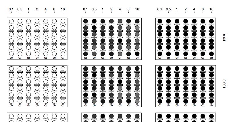
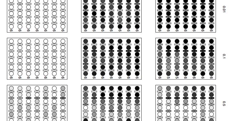
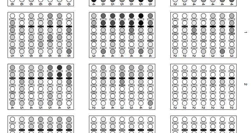
32 29 Figure 1.1: Number of recovered species versus depth of population split. On each subplot, the depth of the split is on the horizontal axis in units of 4N 0 generations; the inferred number of species (median across simulations) is on the vertical axis. Subplots are arranged so that the number of loci sampled increases as one moves down the figure, and the number of individuals sampled per species (population) increases as one moves to the right. Error bars are ± one standard deviation from the simulations. The circles show results from JIST. Circle color shows the proportion of simulations resulting in completely accurate assignment of samples to species, ranging from 0% (white) to 100% (black). Squares show the results from the GMYC approach (Pons et al., 2006), taking the median number of species across simulations; triangles show the results from the GMYC approach with the added constraint of not adding more species than the maximum number possible by JIST (which by default limits results to three or more samples per species), and the dash showing the result from the tree best fitting the GMYC from simulations (error bars not shown for clarity). Lower dashed line shows the correct answer of two species; upper dotted line shows the maximum possible number of species inferable given the sample size by JIST.

33 30

34 31 Figure 1.2: Results in a subdivided population. At the top of the graph is the structure of each metapopulation; sampled demes are in black. The plot shows, at various levels of gene flow, the proportion of times a given deme was returned as a species (darker circles=more frequently returned as a species). The bars show the proportion of times a set of demes was returned as a clade (or a single species) on the species tree; for example, the bar between the first and second populations in model 1 show the proportion of times populations two through four were a clade on the species tree. The number in each box is the median number of species returned.

35 32

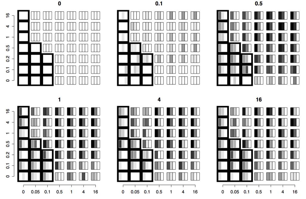
36 33 Figure 1.3: Results from simulating on a four taxon pectinate tree. All times are in units of 4N 0 generations. The x-axis of each plot shows the length of the first (counting from the root) internal edge; the y-axis shows the length of the second internal edge; the number above each plot shows the time from the most recent speciation event to the present. The dark shaded region corresponds to branch lengths where the most probable gene tree does not match the species tree (Degnan and Rosenberg, 2006). Each box is subdivided into three boxes showing results from using a structure weight of 0.1, 0.5, and 0.9, respectively. The shading of each box corresponds to the proportion of simulations where the division of samples into species and species tree were exactly correct (black=all correct, white=none correct).

37 34

38 35 Figure 1.4: Results in a subdivided population with speciation. Migration rate written above each plot; first row of plots has a structure weight parameter value of 0.1, second row of plots has a structure weight of 0.5, and the last row has a structure weight of 0.9. Subplot design as in Figure 1.2

39 36

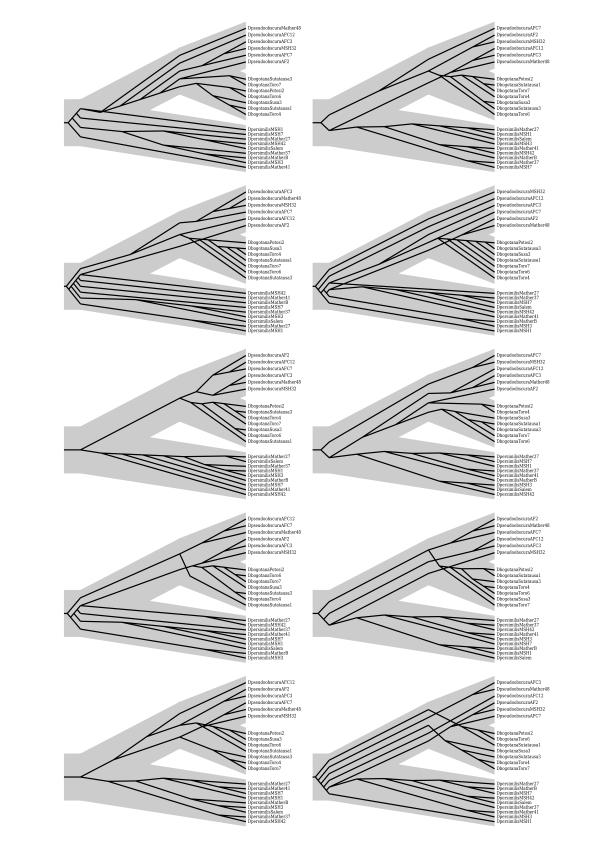
40 37 Figure 1.5: Drosophila data. Shown are gene trees (black trees) from one of the runs resulting in the true species tree (large gray tree), as mapped using PrIMETV (Arvestad, 2006). Note widespread discordance between gene trees and species tree.

41 38

42 39 CHAPTER 2 Mixed model likelihood analysis to estimate Myrmecocystus (Hymenoptera: Formicidae) honeypot ant phylogeny AUTHOR Brian C. O Meara, bcomeara@ucdavis.edu, Center for Population Biology, University of California, Davis. Present address: National Evolutionary Synthesis Center, Durham, NC. ABSTRACT The phylogeny of Myrmecocystus ants is estimated using nine loci, finding that none of the three subgenera are monophyletic, implying repeated evolution of foraging times and particular morphologies. A new partitioned likelihood program, MrFisher, is created from MrBayes to aid analysis of multilocus datasets without assuming priors. Simulations show that using a partitioned likelihood approach in the presence of rate heterogeneity and missing data, as is common in supermatrix analyses, can recover correct branch lengths where non-partitioned likelihood gives predictably biased estimates of branch lengths but the correct topology. KEYWORDS Myrmecocystus, ants, partitions, mixed model, MrFisher

43 40 The analysis of multiple-gene datasets has become increasingly common in phylogenetics due to technological feasibility and theoretical considerations. While individual gene histories may be examined and then combined in a supertree (Sanderson et al., 1998) or related approaches (Edwards et al., 2007; Liu and Pearl, 2007) such data matrices are most commonly examined by concatenating all the genes and then doing one combined supermatrix (de Queiroz and Gatesy, 2007) analysis. To analyze this matrix in a model-based approach, a user may choose to use either a Bayesian approach that allows using different models for different genes but requires making statements about prior beliefs, or a likelihood approach which, with most current implementations, imposes the same model on all genes, regardless of differences in base composition or transition rates between or even within genes. This paper examines and demonstrates the need for partitioned models, modifies the popular program MrBayes to make it into a simulated annealing likelihood search program allowing mixed models models, develops a method for examining conflict between partitions, and uses these tools for investigating the phylogeny and evolution of Myrmecocystus honeypot ants. Myrmecocystus (Wesmael, 1838) ants occur in arid regions of western North America. Their habit of having some workers become swollen repletes to store liquids (a trait convergently evolved in several ant groups) is perhaps their best known trait (see, for example, (Darwin, 1859), Chap. VII, page 239), but they also exhibit such unusual traits within ants as dynamically-allocated territories and ritual combat (Hölldobler, 1976; Hölldobler, 1981). Recent phylogenetic work has shown that the closest relatives to Myrmecocystus are ants of the genera Lasius (Brady et al., 2006; Janda et al., 2004; Moreau et al., 2006). The group was systematically revised by Snelling (Snelling, 1976;

44 41 Snelling, 1982), who split the group into three subgenera. The nominate subgenus consists mostly of golden ants which forage nocturnally; subgenus Eremnocystus are generally small, dark, crepuscular ants; and subgenus Endiodioctes are generally red and black diurnal foragers. A phylogeny based on mtdna (Kronauer et al., 2004) suggested that none of the subgenera are monophyletic. This study adds more loci and species to the analysis to infer a phylogeny needed to study character evolution in the group (O'Meara, 2007a). Bayesian analysis has become quite popular in phylogenetics. This approach has numerous advantages, perhaps most notably integrating over uncertainty in nuisance parameters. A practical advantage is that the most popular program for Bayesian analysis in phylogenetics, MrBayes (Ronquist and Huelsenbeck, 2003), allows mixed models, whereas popular programs for likelihood tree search, such as PAUP (Swofford, 2003) or applications in the PHYLIP package (Felsenstein, 2005), do not support such models (but see RAxML-VI (Stamatakis, 2006), which now includes mixed models and fast likelihood searches). Partitioned models allow different models to be applied to different user-specified partitions of the dataset. Likelihood is consistent (guaranteed to recover the correct tree given enough data) if the correct model is used (Yang, 1994b), but there is evidence that available non-partitioned models may be insufficient. First, in a recent survey (Kelchner and Thomas, 2007) of phylogenetic studies which used the model selection program ModelTest (Posada and Buckley, 2004; Posada and Crandall, 1998), a plurality (43.8%) used the most complex model available, GTR+I+G; the three most complex models available out of 56 total models were used in 63.9% of the studies. Assuming that ModelTest is not systematically overfitting the data, the bunching of

45 42 studies at the maximum complexity end of the model distribution suggests that some of them would have selected even more complex models, had they been available ((Sanderson and Kim, 2000) provide other evidence for this). The few empirical studies of model selection and partitioned models under likelihood suggest that these more complex models often are selected as optimal (Pupko et al., 2002; Wilgenbusch and De Queiroz, 2000). Second, it is commonly observed that different genes, or even different codon positions within a given gene, may differ in important model parameters such as equilibrium base frequencies or transition-transversion rates. Partitioned models, such as those in MrBayes, may address such variation; the models in PAUP and PHYLIP do not. Partitioned models have been shown to be important when estimating branch lengths with full character matrices (Marshall et al., 2006). Partitioned models may also be important when estimating branch lengths in the case of missing data (see below). However, the use of a Bayesian approach in phylogenetics has its own issues. The primary such problem is the importance of the priors. Priors, as a way to incorporate existing information, make sense in many contexts: one might, for example, want to put a low prior probability on re-evolution of a complex morphological trait. In cases where a user does not have strong pre-existing beliefs, uninformative priors may be chosen if available. If not, one can still hope that the information in the data is sufficient to overwhelm any arbitrary prior. However, in the case of branch lengths on trees, this has been shown not to be the case, at least in some situations (Yang and Rannala, 2005). Some users may have strong beliefs regarding these important priors, but many will have no preference regarding whether the prior on branch lengths should be uniform(0,10), exponential(10), exponential(1), or different on internal and external branches, though

46 43 this may dramatically affect the results (Yang and Rannala, 2005). To determine the degree to which researchers use Bayesian approaches in order to incorporate prior knowledge, all 152 papers from 2006 in Molecular Phylogenetics and Evolution which used MrBayes to get Bayesian estimates of trees were examined. Of these, only 23.7% even mentioned the substitution model or branch length priors and only 3.3% (just 5 papers) modified these from the default values (and often just modified them based on likelihood-optimized values calculated for the same dataset using ModelTest or MrModelTest (Nylander, 2004)). Evidently, incorporating individual prior beliefs about molecular evolution in their group is not a primary motivation for researchers choosing to use a Bayesian approach. METHODS Taxon sampling and molecular data Mesosomas and limbs of ethanol-preserved Myrmecocystus samples and outgroup species were extracted using Qiagen tissue extraction kits (heads and gasters were vouchered). For two samples for which consumable specimens were not available, a nondestructive extraction was performed. Outgroup taxa were Lasius subumbratus, L. niger, Lasius californicus, and Formica moki, used as an outer outgroup. Where available, outgroup sequences came from published sequences from (Brady et al., 2006); all ingroup sequences were generated de novo. All subgenera and species groups of Myrmecocystus have been sampled for this study; detailed information about collections, sequencing results, and ranges is available at In this study, sequences from nine loci were used: Cytochrome

47 44 oxidase I, wingless, enolase, long wavelength rhodopsin, arginine kinase, elongation factor 1-alpha ortholog 2, UV opsin, abdominal A, and dynamin. Pilot work also sequenced 18S, 28S, TPI, ITS2, and elongation factor 1-alpha ortholog 1 but these genes were found to be unsuitable (too unalignable, character-poor, or difficult to sequence in some taxa) and so were not pursued for this study. Primers and reaction conditions are in the supplementary information. Not all genes were sampled for all taxa (primer failure, lack of variation in some genes), but the resulting supermatrix is rather full (74.5% of all positions in the matrix have a nucleotide, despite inclusion of introns with indels and missing genes for some taxa), especially for genes found to be phylogenetically useful. Twenty-one taxa have sequence from all nine loci, five more have sequence from eight loci, and the remaining taxa have five or more loci sampled (see supplementary information). The set of taxa easily form a grove sensu (Ane et al., 2006). All new sequences are deposited in Genbank as EU EU ABI chromatograms were analyzed by Pregap4 and edited in Gap4, both part of the Staden 1.60 package (Staden et al., 2000). Sections with base confidence below were excluded, unless inspection of chromatograms showed an obvious sequencing artifact with the correct reading obvious or the correct reading was unambiguous in one or more overlapping chromatograms. Cytochrome oxidase sequences showed evidence of some sequences coming from nuclear copies of mitochondrial sequence (NUMTs, Lopez et al., 1994), such as mismatch between sequences generated from overlapping primer pairs, and in one case, a five base pair deletion. Sequence chromatograms were examined closely for potential NUMTs with evidence used of indels (one case), and less certainly, heterozygosity within

48 45 a read (multiple peaks at a site) or conflict between overlapping regions. Any suspected regions were excluded from analysis. Sequences for each locus were aligned with MAFFT (Katoh et al., 2005) using the ginsi option to maximize accuracy, then the alignment was refined by eye, hiding taxon names to reduce bias at this stage. Sequences were then concatenated using a Perl script. Partition sets were created using the web application ModelPartition, which can create partition sets for MrBayes and MrFisher (O'Meara, 2007b). Phylogenetic Analysis: A New Program MrBayes (Ronquist and Huelsenbeck, 2003) is a fast, open-source, C program for the inference of phylogenetic trees using Bayesian inference. It can use a range of data types, including nucleotides, amino acids, restriction sites, and even morphological characters with a wide variety of models, including mixed (partitioned) models, with and without a molecular clock enforced. It uses a Metropolis-coupled Markov Chain Monte Carlo algorithm (MC 3 ) to estimate posterior probabilities of topologies, branch lengths, and nuisance parameters. Briefly, this entails a walk through parameter space by proposing moves (changes in parameter value or the tree), with moves resulting in better scores (likelihood times prior) being accepted all the time, and moves resulting in worse scores being taken a proportion of the time (the worse a move is, the lower the chance of accepting it). Several heated chains are used: heating just makes the likelihood surface flatter, ideally allowing moves across valleys of worse parameter values by making them relatively less bad than they would be in an unheated chain. Periodically, the states of the cold and heated chains are examined and occasionally the heating factor of the chains

49 46 may be swapped, so that a heated chain that has successfully moved across a valley to a different part of tree space may become unheated and thus used for acquiring samples (two heated chains of different temperatures may also be swapped). Simulated annealing (Kirkpatrick et al., 1983) has been applied to phylogenetic tree search multiple times (Barker, 2004; Salter and Pearl, 2001; Stamatakis, 2005). It is an optimization technique, not an integration technique (like MC 3 ), intended to find a global optimum in a situation where there may be multiple local optima. It works by always accepting moves to better states but sometimes accepting moves to worse states. Unlike MC 3, where the probability of moves to a worse state just depends on the magnitude of the difference, with simulated annealing both the magnitude of the difference and current value of a control parameter matter. This control parameter decreases during a search, making a move to a particular worse state more likely earlier in a search. The rate at which this occurs is known as the cooling schedule, in analogy to annealing in metallurgy, where cooling a material slowly allows atoms to find low energy placements and thus increase crystal size (a more familiar example of this sort of process is the creation of crystals through precipitation of solutes from an evaporating solution: the more slowly evaporation occurs, the larger the resulting sizes of the crystals formed). The control parameter and cooling schedule used in MrFisher are the same as those suggested by Salter and Pearl (2001), with the exception of using a tree from an initial search rather than a neighbor-joining tree to get a starting likelihood value in parameterizing the control parameter. An MC 3 search in MrBayes stops at a user-determined number of generations or after the standard deviations of posterior probabilities of clades between two or more runs

50 47 drops below a user-determined threshold. The goal is to run long enough both to move the chain to a point of convergence (where parameter values are sampled based on their posterior probabilities, not due to being close to the starting point in parameter space) and then to provide sufficiently precise and accurate posterior probability estimates. A simulated annealing search seeks the single optimum combination of topology, branch lengths, and nuisance parameters, not the posterior distributions of all these parameters. Users may set a stopping criterion based on total number of attempted moves or based on the total number of moves elapsed since the last improvement in likelihood. The default behavior of MrFisher for a tree with N taxa and K model parameters is to stop after N 3 K generations without an improvement. Phylogenetic Analysis: Combined Analysis The range of possible models is vast. Within each partition set, just varying the number of free DNA instantaneous transition rates (1, 2, or 6) and the model of rate heterogeneity (equal rates, gamma-distributed rates, the proportion of invariant sites, or allow gamma and invariant sites) results in 12 different models within each partition (for reviews of substitution models, see Felsenstein (2004) and Yang (2006)). The maximum reasonable partition set is to have different partitions for each codon position of each gene, plus one partition for each intron; in this dataset, this would result in 33 partitions. Trying all combinations of substitution models (i.e., COI first codon position having an HKY+G model, all other partitions having an F81 model, is just one combination) would result in possible combinations (over ) for just this one partition set, and there are several other reasonable partition sets. Thus, to determine the optimal partitioning and

51 48 model scheme, a set of possible partitions was devised. For each set of characters placed in one partition, ModelTest (Posada and Crandall, 1998) was run with PAUP to return the optimal substitution model for that set of characters under the AIC c (since PAUP can implement more models than MrFisher, the model occurring in both programs with the highest AIC c was the one chosen). This substitution model was then used for that set of characters anytime they were in a partition (for example, the optimal model for COI was GTR+I+G; this was used when characters were partitioned by gene, as well as when characters were partitioned by genome, since in both cases, all the COI characters made up one partition; the optimal model for COI third codon position sites was HKY+G, and so this model was used whenever these sites constituted a partition). Each partition with the assigned substitution models was then run in MrFisher in a full tree search to estimate the likelihood and therefore AIC c of each partition. At this step, it was noticed that some of the parameter estimates for some of the nuisance parameters in some of the partitions were extreme (such as transition/transversion ratios greater than 1,000,000), and this tended to correlate with searches where the likelihood scores varied dramatically between runs. This was traced back to partitions where the model chosen by AIC c (which takes into account small sample size) was more complex than the simple F81 but the relevant partition had very few variable sites. For example, the second codon position of Abdominal A had 210 sites (used as the sample size in AIC c calculations), of which the sole variable site was not parsimony-informative. The optimal model according to AIC c was HKY (two substitution types, unequal base frequencies), followed by F81 (!AIC c =0.33; one substitution type, unequal base frequencies). The most complex model available, GTR+I+G (!AIC c = 12.18), was ranked higher than the simplest model, JC

52 49 (!AIC c = 71.01). [Likelihood ratio tests selected F81]. While AIC c does take into account sample size, exactly how to calculate this sample size is not well understood in phylogenetics (Posada and Buckley, 2004), though the standard practice is to just take the number of characters, ignoring number of taxa or the number of variable characters. To prevent possible overparametrization, the models for each partition were chosen again with a slightly modified ModelTest, this time using the number of variable characters as the sample size, increasing the recorded number of free parameters of each model (K) by one (as the relative rate for each partition is a parameter which must be estimated in a partitioned search), and allowing ModelTest to ignore models for which there were not more samples than parameters rather than aborting the analysis of all models in such a case (a situation which can occur if, for example, examining a GTR+I+G model with only 7 variable sites). Using this new procedure, those partitions which returned extreme parameter estimates under the original models were assigned simpler models; several other partitions were also assigned simpler models (this was especially common for partitions where the number of variable sites was less than twice the number of free substitution model parameters in the original model). The search for the optimal partition set was re-run with the new substitution models; each partition set was run five times, with stopping determined by the MrFisher futile generation default or 200M generations, whichever occurred first. The optimal model was used with MrFisher in a heuristic search. Searches starting from 50 different initial conditions were run. The phylogram with highest likelihood over all the runs was used with non-parametric rate smoothing in r8s 1.71 (Sanderson, 1997; Sanderson, 2003) and a maximum estimate of the Lasius-

53 50 Myrmecocystus split from work on the ant AToL team (S. Brady, pers. comm.) of MY to make the tree ultrametric and provide a rough calibration. A partitioned bootstrap search was performed. Under normal bootstrapping, the proportion of characters in each partition could change (for example, for the smallest partition of 64 sites in this dataset, ten percent of the replicates will have " 51 or # 77 of those sites represented). By sampling characters with replacement from within each partition, the variation in representation of each partition is removed, which may better mirror reality (in a real replicate dataset, the ratio of the numbers of first and second codon positions in a gene would not change), while not dramatically changing the probability that a given site will be absent from the pseudoreplicate dataset (for example, a site in the 64 site partition has a 36.5% chance of being omitted from a partitioned bootstrap pseudoreplicate dataset and a 36.8% chance of being omitted from a regular bootstrap dataset). In practice, this also guards against the extremely low probability event of creating a dataset with no samples from a particular partition and then trying to estimate model parameters for that partition. Substitution model parameters for the search were fixed based on those from the likeliest tree search results. Two hundred bootstrap replicates, each starting from five different trees, were performed in MrFisher. As a check, 200 bootstrap replicates, each starting from ten random taxon addition starting trees and using a GTR+I+G model with parameter values fixed on a neighbor-joining tree, were performed in PAUP. A given bootstrap replicate may return more than one equally-likely tree; to avoid having to deal with tracking tree weights in future analyses, only the first tree from each replicate was used.

54 51 With any analysis based on sets of characters which may have different histories (such as different loci), one concern is whether all the character sets agree on the resolution; another concern is identifying which character sets provide most of the signal in the analysis. In parsimony, this question is often addressed using partitioned Bremer support (Baker and DeSalle, 1997); a likelihood analogue, partitioned likelihood support (Lee and Hugall, 2003), has also been developed. In either approach, for each bipartition on the optimal tree, a new tree search is performed with the constraint that the resulting tree not have that bipartition. The score of each character set on this new tree is compared to the corresponding score on the original tree: character sets that favor a different bipartition than the one on the unconstrained-search tree may get better scores under the constrained search, while character sets that strongly favor the unconstrained-search bipartition will have much worse scores. One disadvantage of this approach is that it requires a thorough but constrained tree search for each internal edge of the original tree. This can be a time-consuming process. Another practical concern is that MrFisher cannot do searches with reverse constraints. Forcing each character set to be fit to the same alternate tree may also obscure some conflict. For example, if half the character sets mildly favor tree A over tree B and strongly favor tree B over tree C (A<B<<C, smaller is better), and the other character sets mildly favor tree C over tree B and strongly favor tree B over tree A (C<B<<A), the optimal tree for all characters may be tree B. Under a constrained search preventing the return of tree B, either tree A or tree C may be returned. If the returned tree is A, then the first sets of characters are seen to fit this tree slightly better and so conflict with tree B, while the second sets of characters are seen to fit this tree much worse and so strongly support tree B. In fact, all the sets of the

55 52 characters conflict with tree B, but some mildly favor A and some mildly favor C. To deal with these practical and theoretical concerns, a different approach, nearest neighbor interchange branch support (NNIBS), was developed. For each internal edge, the two topologies resulting from swapping two of the branches on either side of the edge (doing an NNI swap across that edge) are created. Each character set was fit to these two trees and the original tree (estimating branch lengths for each tree just using that character set) using PAUP with the chosen model for each character set (these models correspond to the ones used in MrFisher; this approach could not be done in that program because MrFisher inherited a bug from its MrBayes ancestor that appears to prevent the loading of trees as starting trees for just model-fitting). The lesser of the differences between the original tree and the two new trees was taken as the NNIBS score for that character set for that edge. Partitioning with Missing Data Multi-locus datasets are often missing sequences for particular taxa for particular genes, due to sequencing failure, budget issues, or other factors. This is especially common with supermatrix approaches, which create often very sparse matrices from existing data (i.e., Driskell et al., 2004). The effect of missing data on reconstructing the correct topology has been examined several times, and a basic conclusion of this work is that missing data is not a problem as long as there is a sufficiently informative dense portion of the matrix (reviewed by Wiens (2006)). However, the effect of missing data, with the gaps non-randomly distributed with respect to locus, as one commonly encounters with empirical datasets, on branch length estimates has been little-examined.

56 53 Branch lengths are of critical importance in phylogenetics: almost every model-based method for understanding evolution, whether in estimating speciation and extinction rates (Nee et al., 1994), using independent contrasts to look at character correlations (Felsenstein, 1985), or looking at discrete character transition rates (Pagel, 1994), generally requires a tree with branch lengths (unless uniform branch lengths can be assumed under a speciational model of trait evolution with no extinction). Timecalibrating trees also generally requires having initial branch lengths. While there are methods for inventing branch lengths when ones based on data are not used (Grafen, 1989; Purvis, 1995), the performance of partitioned and non-partitioned likelihood in recovering accurate branch lengths in the presence of missing data is of great import. Two approaches were used to investigate this: the optimization of a branch on a simple tree with varying amounts of fast or slow sites deleted from one taxon, and the simulation of data with two rates on a moderate-sized tree, deletion of some of this data, and reconstruction of the trees. First, a model was constructed consisting of an ultrametric three taxon tree (A:2,(B:1,C:1):1), with known edge lengths; data was to be two loci of equal length and possibly unequal substitution rates (and with a simple twostate symmetric model), and a proportion m of the second locus was to be deleted from taxon C. Equations were written for the probability of each site pattern (000, 001, 010,, 111, 00?, 01?, 10?, 11?) under a model with proportion m and substitution rates u i and u ii. Equations were written for the likelihood of each site pattern under a single rate model but with the length of the edge leading to C an unknown parameter t in the model. The likelihood of an infinitely long dataset under the single rate model, estimating t, is then just proportional to the product of the site pattern likelihoods, each raised to the

57 54 probability of that site pattern given the true model. The estimate of t under various combinations of rate parameters and missing data values was evaluated using R (2007). Second, data were simulated on a rooted 32-taxon balanced tree with all edge lengths equal. For each simulation, two loci, of 2000 characters each, were simulated under the same GTR+I+G model (parameterized based on values estimated from the COI Myrmecocystus dataset) using Seq-Gen (Rambaut and Grassly, 1997), but one locus had 10 times the substitution rate as the other (done by scaling branch lengths on the tree). The data for the fast locus was deleted for six taxa (the 1 st, 3 rd, and 13 th -16 th taxa) and for the slow locus was deleted for a different six taxa (the 17 th, 19 th, and 29 th -32 nd taxa). Data was analyzed under a GTR+I+G substitution model in MrFisher, with the two loci allowed to have different overall rates (but the same linked GTR+I+G settings) in a partitioned model and the same rate in a non-partitioned model. Results from 25 simulations and analyses are presented here. This investigates how partitioned and nonpartitioned likelihood perform in branch length estimation in realistic data sets. RESULTS Selected models The optimal model, whether using AIC c with sample size of the number of characters or sample size the number of variable characters, allowed each codon position and the introns of each locus to have their own substitution model; this partition set had 33 partitions and 159 free substitution model parameters (Table 2.1). The second best model (!AIC c =78.8) was only the fifth most complex, with just seven partitions and 51 free parameters. The model with all the sequences in one partition had an AIC c score

58 worse than the best partitioned model; a difference greater than 10 is generally taken to indicate essentially no support for the worse model (Burnham and Anderson, 2002). Though the model selected had the maximum number of partitions, it was not the most complex model possible, which would have applied a GTR+I+G model to each partition, as well as its own rate, which would have resulted in 362 free parameters, over twice the number present in the chosen model. As the dataset was more finely partitioned, smaller partitions had simpler models applied; 17 of 33 regions in the chosen model were assigned an F81 substitution model, for example. Myrmecocystus Tree The topology of the tree with best likelihood overall was found in 27 of 50 runs. This tree (Figure 2.1) differed from that of (Kronauer et al., 2004): in the Kronauer et al. tree, their two species from subgenus Myrmecocystus did not form a clade, but in this analysis, those two species formed a clade with three other subgenus Myrmecocystus species. However, the subgenus is still not a clade, as M. pyramicus is sister to a clade of three Eremnocystus species. Endiodioctes is rendered paraphyletic due to insertion of M. yuma in the group (also observed by Kronauer et al.); the Eremnocystus species M. creightoni is sister to that entire clade (the Kronauer et al. study lacked resolution for this question). Bootstrap support for many of the branches of the tree, using both MrFisher and PAUP, was moderate. A plot of bootstrap support versus length of the branch reveals that most of the poorly-supported branches are under 2 million years in duration, assuming the MY calibration is accurate.

59 56 Conflict Between Partitions The NNIBS test results (Table 2.2) reveals that much of the signal came from third codon positions of COI and nuclear introns, though nuclear exons also contributed important signal. While there was some conflict between partitions, there was not a strong pattern of conflict between nuclear and mitochondrial signals, suggesting but not proving that the returned phylogeny is not a result of undiscovered NUMTs. Two edges had overall negative NNIBS scores: this can occur if the returned topology is a compromise between conflicting data. Missing Data and Partitioning The first approach (Figure 2.2) shows that with no missing data, but two different substitution rates, likelihood reconstructs the length of the branch leading to taxon C correctly. If the substitution rates are equal, the length is also reconstructed correctly for any amount of data missing from the second locus, indicating that missing data alone does not lead to branch length mis-estimation. However, if the second locus is faster than the first, missing data from that locus for taxon C leads likelihood under a single rate model to underestimate the length of that branch (and the opposite happens for a slower rate). The second approach shows the same kind of result. Omission of the fast locus for some taxa results in an underestimate of their branch length using the nonpartitioned model; the opposite branch length bias occurs, though with less extreme changes in branch length, with omission of the slow locus (Figure 2.3). A one-sided (in the predicted direction) paired sample t-test with unequal variances to compare sister groups differing

60 57 in missing sequence for equal branch lengths finds that on the nonpartitioned searches, the groups lacking the fast gene have significantly shorter branches (P<0.001) than their sisters, while the groups lacking the slow gene have significantly longer branches (P<0.05) than their sister groups. On the partitioned searches, only one comparison between a taxon missing fast sites and its sister is marginally significant (P=0.026); the rest are insignificant (P>0.3). With a Bonferroni correction, the partitioned search has no significant differences, but all three comparisons between a subtree missing fast sites and its sister remain significant (P<0.01) for the nonpartitioned search, as does the comparison between the four-taxon clade missing slow sites and its sister (P= ) but not between the single missing-slow taxa and their sisters. DISCUSSION Additional taxa and loci for Myrmecocystus phylogeny have led to greater resolution and a somewhat different tree from previous research (Kronauer et al., 2004). Lack of monophyly of any of the subgenera suggest that the associated foraging time and morphological traits have changed multiple times [see accompanying paper]. When revising the group, Snelling speculated that there were two major divisions in the group, the first between the nominate subgenus and the remaining taxa, and the second between Endiodioctes and Eremnocystus. The results from this analysis approximate this. A clade of subgenus Myrmecocystus ants is sister to the rest of the ants, which includes one other ant of the nominate subgenus, M. pyramicus. There is indeed a split between a clade of Endiodioctes ants (plus the Eremnocystus species M. yuma) and a grade of Eremnocystus ants (plus M. pyramicus). However, while Snelling postulated that Eremnocystus are

61 58 derived from Endiodioctes, presumably rendering the latter paraphyletic, the reverse is recovered (with the exception of M. yuma). Further investigation of Myrmecocystus evolution using this tree is pursued in an accompanying study (O'Meara, 2007a). Using a single model of evolution when dealing with data sets with various rates of evolution and missing data can significantly bias reconstructed branch lengths, even when the correct topology is returned (as in the simulations using the 32-taxon balanced tree). Taxa lacking fast regions (and thus having a greater proportion of slow sites) are reconstructed as having branches that are too short, while taxa lacking slow regions are assigned longer branches. Partitioned analysis appears to correct this, if the partitions are assigned correctly (assigning sites with different rates to different partitions). Traditional ways of dealing with site rate heterogeneity, such as using a discrete gamma approximation (Yang, 1994a) or a proportion of invariant sites, both of which were used in the DNA simulation, do not correct for this bias: they calculate likelihoods by summing probabilities over the same set of rates to all sites rather than assigning particular rates to particular sites. Site-specific models, which are essentially the partitioned likelihood model used here, have more success. This study only examined the effect of different rates of evolution at different sites with missing data; different substitution model parameters at different sites are also likely to induce incorrect branch length estimates, and may require partitioned models to correct. This study has used multiple loci under a complex model of evolution to infer the phylogeny of Myrmecocystus ants, revealing that foraging time has repeatedly changed in this group. The accompanying study uses this information to infer the effect of these changes on character evolution.

62 59 PROGRAM AVAILABILITY Source code and binaries of MrFisher and the modified version of ModelTest are both available at as are relevant Perl scripts used in this study. ACKNOWLEDGEMENTS Computing resources were provided by the Evolution and Ecology department at the University of California, Davis and by the National Evolutionary Synthesis Center and Duke University. John Huelsenbeck and Frederick Ronquist published MrBayes under an open source license, permitting the modifications here, and wrote clean, wellcommented code making the modifications feasible. Funding for BCO came from the Center for Population Biology, a National Science Foundation Graduate Research Fellowship, and UC Davis; research funding came from a National Science Foundation Dissertation Improvement Grant, UCD Center for Biosystematics research grants, UCD Center for Population Biology research awards, and UC Jastro-Shields research scholarships. Phil Ward gave invaluable guidance and mentorship throughout this study, in ways as various as organizing collecting trips, training in the craft of myrmecology, and suggesting new approaches to wet lab work. Further advice came from Mike Sanderson and Michael Turelli. Specimens were donated by Phil Ward, Alex Wild, Robert Johnson, and David Holway.

63 60 DATA DEPOSITION Sequences are deposited in Genbank, accession numbers EU EU Topologies and aligned sequence data are in TreeBase, study number. TreeBase prohibits submission of trees with branch length information; thus, trees from this study with branch length information are available at and also will be deposited in an appropriate repository once one is available.

64 R: A Language and Environment for Statistical Computing. R Foundation for Statistical Computing. Ane, C., O. Eulenstein, R. Piaggio-Talice, and M. J. Sanderson Groves of phylogenetic treestechnical Report Department of Statistics, University of Wisconsin, Madison, Wisconsin. Baker, R. H., and R. DeSalle Multiple Sources of Character Information and the Phylogeny of Hawaiian Drosophilids. Systematic Biology 46: Barker, D LVB: parsimony and simulated annealing in the search for phylogenetic trees. Bioinformatics 20: Brady, S. G., T. R. Schultz, B. L. Fisher, and P. S. Ward From the Cover: Evaluating alternative hypotheses for the early evolution and diversification of ants. Proceedings of the National Academy of Sciences 103: Burnham, K. P., and D. R. Anderson Model selection and multimodel inference : a practical information-theoretic approach. Springer, New York. Darwin, C On the Origin of Species by Natural Selection. Murray, London, United Kingdom. de Queiroz, A., and J. Gatesy The supermatrix approach to systematics. Trends in Ecology & Evolution 22: Driskell, A. C., C. Ane, J. G. Burleigh, M. M. McMahon, B. C. O'Meara, and M. J. Sanderson Prospects for building the tree of life from large sequence databases. Science 306: Edwards, S. V., L. Liu, and D. K. Pearl High-resolution species trees without concatenation. Proceedings of the National Academy of Sciences 104:

65 62 Felsenstein, J Phylogenies and the Comparative Method. The American Naturalist 125:1-15. Felsenstein, J Inferring Phylogenies. Felsenstein, J PHYLIP version 3.6. Distributed by the author. Department of Genome Sciences, University of Washington, Seattle. Grafen, A The Phylogenetic Regression. Philosophical Transactions of the Royal Society of London. Series B, Biological Sciences 326: Hölldobler, B Tournaments and slavery in a desert ant. Science 192: Hölldobler, B Foraging and spatiotemporal territories in the honey ant Myrmecocystus mimicus Wheeler (Hymenoptera: Formicidae). Behav. Ecol. Sociobiol. 9: Janda, M., D. Folkova, and J. Zrzavy Phylogeny of Lasius ants based on mitochondrial DNA and morphology, and the evolution of social parasitism in the Lasiini (Hymenoptera: Formicidae). Molecular Phylogenetics and Evolution 33: Katoh, K., K. Kuma, H. Toh, and T. Miyata MAFFT version 5: improvement in accuracy of multiple sequence alignment. Nucleic Acids Research 33: Kelchner, S. A., and M. A. Thomas Model use in phylogenetics: nine key questions. Trends in Ecology & Evolution 22: Kirkpatrick, S., C. D. Gelatt Jr, and M. P. Vecchi Optimization by Simulated Annealing. Science 220:671.

66 63 Kronauer, D. J. C., B. Holldobler, and J. Gadau Phylogenetics of the new world honey ants (genus Myrmecocystus) estimated from mitochondrial DNA sequences. Molecular Phylogenetics and Evolution 32: Lee, M. S. Y., and A. F. Hugall Partitioned Likelihood Support and the Evaluation of Data Set Conflict. Systematic Biology 52: Liu, L., and D. K. Pearl Species Trees from Gene Trees: Reconstructing Bayesian Posterior Distributions of a Species Phylogeny Using Estimated Gene Tree Distributions. Systematic Biology 56: Lopez, J. V., N. Yuhki, R. Masuda, W. Modi, and S. J. O'Brien Numt, a recent transfer and tandem amplification of mitochondrial DNA to the nuclear genome of the domestic cat. Journal of Molecular Evolution 39: Marshall, D. C., C. Simon, and T. R. Buckley Accurate Branch Length Estimation in Partitioned Bayesian Analyses Requires Accommodation of Among-Partition Rate Variation and Attention to Branch Length Priors. Systematic Biology 55: Moreau, C. S., C. D. Bell, R. Vila, S. B. Archibald, and N. E. Pierce Phylogeny of the Ants: Diversification in the Age of Angiosperms. Pages American Association for the Advancement of Science. Nee, S., E. C. Holmes, R. M. May, and P. H. Harvey Extinction Rates can be Estimated from Molecular Phylogenies. Philosophical Transactions: Biological Sciences 344: Nylander, J. A. A MrModeltest v2. Evolutionary Biology Centre, Uppsala University.

67 64 O'Meara, B. C. 2007a. Coevolution of foraging time and morphology in Myrmecocystus (Hymenoptera: Formicidae). in prep. O'Meara, B. C. 2007b. ModelPartition. Pagel, M Detecting Correlated Evolution on Phylogenies: A General Method for the Comparative Analysis of Discrete Characters. Proceedings: Biological Sciences 255: Posada, D., and T. Buckley Model selection and model averaging in phylogenetics: advantages of akaike information criterion and bayesian approaches over likelihood ratio tests. Systematic biology 53: Posada, D., and K. A. Crandall MODELTEST: testing the model of DNA substitution. Bioinformatics 14: Pupko, T., D. Huchon, Y. Cao, N. Okada, and M. Hasegawa Combining Multiple Data Sets in a Likelihood Analysis: Which Models are the Best? Mol Biol Evol 19: Purvis, A A Composite Estimate of Primate Phylogeny. Philosophical Transactions: Biological Sciences 348: Rambaut, A., and N. C. Grassly Seq-Gen: an application for the Monte Carlo simulation of DNA sequence evolution along phylogenetic trees. Bioinformatics 13: Ronquist, F., and J. P. Huelsenbeck MrBayes 3: Bayesian phylogenetic inference under mixed models. Bioinformatics 19: Salter, L. A., and D. K. Pearl Stochastic Search Strategy for Estimation of Maximum Likelihood Phylogenetic Trees. Systematic Biology 50:7-17.

68 65 Sanderson, M. J A nonparametric approach to estimating divergence times in the absence of rate constancy. Molecular Biology and Evolution 14: Sanderson, M. J r8s: inferring absolute rates of molecular evolution and divergence times in the absence of a molecular clock. Bioinformatics 19: Sanderson, M. J., and J. Kim Parametric phylogenetics? Systematic Biology 49: Sanderson, M. J., A. Purvis, and C. Henze Phylogenetic supertrees: assembling the trees of life. Trends in Ecology & Evolution 13: Snelling, R. R A revision of the honey ants, genus Myrmecocystus (Hymenoptera: Formicidae). Nat. Hist. Mus. Los Angel. Cty. Sci. Bull. 24: Snelling, R. R A revision of the honey ants, genus Myrmecocystus, first supplement (Hymenoptera: Formicidae). Bull. South. Calif. Acad. Sci. 81: Staden, R., K. F. Beal, and J. K. Bonfield The Staden package, Methods Mol. Biol 132: Stamatakis, A An Efficient Program for Phylogenetic Inference Using Simulated Annealing. Parallel and Distributed Processing Symposium, Proceedings. 19th IEEE International:198b-198b. Stamatakis, A RAxML-VI-HPC: maximum likelihood-based phylogenetic analyses with thousands of taxa and mixed models. Bioinformatics 22: Swofford, D. L PAUP*. Phylogenetic Analysis Using Parsimony (*and Other Methods). Version 4., version 4.0b10. Sinauer Associates. Wesmael, C Sur une nouvelle espèce de fourmi du Mexique. Bull. Acad. R. Sci. B.-Lett. Brux. 5:

69 66 Wiens, J. J Missing data and the design of phylogenetic analyses. Journal of Biomedical Informatics 39: Wilgenbusch, J., and K. De Queiroz Phylogenetic Relationships Among the Phrynosomatid Sand Lizards Inferred from Mitochondrial DNA Sequences Generated by Heterogeneous Evolutionary Processes. Systematic Biology 49: Yang, Z. 1994a. Maximum likelihood phylogenetic estimation from DNA sequences with variable rates over sites: Approximate methods. Journal of Molecular Evolution 39: Yang, Z. 1994b. Statistical Properties of the Maximum Likelihood Method of Phylogenetic Estimation and Comparison with Distance Matrix Methods. Systematic Biology 43: Yang, Z Computational Molecular Evolution. Oxford University Press. Yang, Z., and B. Rannala Branch-Length Prior Influences Bayesian Posterior Probability of Phylogeny. Systematic Biology 54:

70 67 Figure 2.1: Myrmecocystus phylogeny generated by MrFisher. Numbers above branches are MrFisher / PAUP bootstrap support; numbers below branches are labels corresponding to labels in Table 2.2. The scale bar represents two million years based on a calibration from the ant AToL group. The outer outgroup, Formica moki, is omitted from this plot (it was pruned before making the tree ultrametric). Letters following brackets represent subgenus: M=Myrmecocystus, R=Eremnocystus; the remainder of the Myrmecocystus taxa are in subgenus Endiodioctes. The embedded plot shows the correlation of branch length and bootstrap proportion.

71 68

72 69 Figure 2.2: Effect of missing data on reconstructed branch length, simple case. Solid line corresponds to the second locus having a substitution rate 75% that of the first locus; dashed line with equal rates; and dotted line corresponds to a substitution rate 125% of the first locus. The true length of t, the branch leading to taxon C in the tree (A,(B,C)), is 1 in all simulations.

73 70

74 71 Figure 2.3: Data for two 2,000 bp loci with a tenfold rate difference were generated by simulating on a balanced 32-taxon tree with uniform branch lengths. For taxa shown in red, sequence for the fast locus was deleted; blue taxa lack the slow locus. Branch lengths on the left tree are averages across 25 simulated datasets analyzed by MrFisher under a non-partitioned model; branch lengths on the right tree are averages across 25 simulations analyzed using a model allowing the first and second loci to have different rates. Asterisks above and below branches indicate P-values for equal total branch length (using a t-test on the trees from the simulations) of the two subtrees descended from that branch before and after Bonferroni correction: P<0.001 = ***, P<0.01 = **, P<0.05 = *.

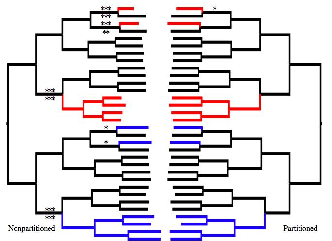
75 72

76 73 Table 2.1: Partitions and selected models. Shown are the number of partitions in a given model, the number of free substitution parameters for that model, and the!aic c score for that model, followed by the assignment of sites to partitions (sets of sites sharing the same symbol are in the same partition). The second part of the table shows the model selected for each partition using the modified version of ModelTest.

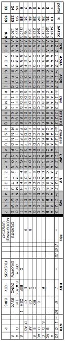
77 74

78 75 Table 2.2: Nearest neighbor interchange branch support (NNIBS). Positive values indicate that the character set has a better score under the recovered tree than under a tree with the bipartition replaced by an NNI swap along the relevant edge. Values equal to zero are omitted for clarity. Edge numbers correspond to numbers under branches in Figure 2.1.

79 76

80 77 CHAPTER 3 Character evolution in Myrmecocystus honeypot ants AUTHOR Brian C. O Meara, bcomeara@ucdavis.edu, Center for Population Biology, University of California, Davis. Present address: National Evolutionary Synthesis Center, Durham, NC. ABSTRACT Evolution of foraging time and coevolution of behavior and morphology in Myrmecocystus ants is examined. New models for reconstructing discrete states along branches of a tree and for examining continuous trait evolution and coevolution with discrete traits are developed and implemented. Foraging transitions between diurnal and nocturnal foraging evidently go through crepuscular intermediates. There is some evidence for increased rates of morphological character evolution associated with changes in foraging regime, but little evidence for particular optimum values for morphological traits associated with foraging. KEYWORDS Brownie Myrmecocystus, comparative methods, Brownian motion, Ornstein-Uhlenbeck,

81 78 Selection acts on both behavior and morphology of organisms. These traits can thus be expected to occasionally coevolve: an addition of a new prey item to the diet may shift selection pressures on feeding structures; the evolution of toxic skin may shift the optimal behavioral response to a potential predator. There are several tree-based approaches for examining such relationships between two traits, such as independent contrasts (Felsenstein, 1985) for looking at correlation of state between two continuous traits and other methods for examining correlations of state between two discrete traits (Maddison, 1990; Pagel, 1994). This paper extends the range of such models to allow examination of how state of a discrete character may affect the rate of evolution of a continuous character, how changes in the state of a discrete character may affect the rate of evolution of a continuous character, and how the state of a discrete character affects the optimal value of a continuous character. It also implements more discrete character models than have been available in the past, in the service of understanding how behavior (foraging time) and morphology coevolve in a clade of desert ants. Myrmecocystus (Wesmael, 1838) honeypot ants occur in arid regions of western North America. Members of this clade (Kronauer et al., 2004; O'Meara, 2007) are wellknown for their habit of forming repletes: workers with swollen gasters used for liquid storage. They are generalist foragers, collecting Hemipteran honeydew, flower nectar, dead insects, occasionally live prey, and sometimes stealing food from other ant species (Cole et al., 2001; Hölldobler, 1981; Hölldobler, 1986; Snelling, 1976; Snelling, 1982). They differ most notably in foraging time. In a given location, there may be one species that only forages diurnally in hot sun, another species that only forages in the cool desert nights, and a third species that emerges only at dawn and dusk to forage in pulses

82 79 (Snelling, 1976). They also differ in gross morphology: diurnal species are often red and black ants of medium size, nocturnal species are gold to brown ants of variable size, and crepuscular ants are often black and small. There are also predictions regarding how foraging time affects other aspects of morphology. In ants, long legs allow faster walking speeds (Zollikofer, 1994) and greater distance between the body and the substrate. Thus, diurnal Myrmecocystus, which forage at substrate temperatures up to 60 C and which show behaviors of running from patches of shade to shade quickly and raising their body above hot substrates (Snelling, 1976), may be under selection for longer legs than species that avoid such temperatures. Similarly, pilosity (hair coverage) has been suggested to aid in insulating diurnal ants from their hot environment (Snelling, 1976), and so we may postulate that diurnal ants should have more hair. There may also be an effect of environment on the rate of character evolution: perhaps diurnal ants are constrained to have long legs and hairy bodies, but other ants are free to explore various optima for these traits and so have a higher rate of evolution for them. Diurnal desert foraging may be a hard strategy to adopt due to physiological constraints: for example, though some Endiodioctes forage at surface temperatures of 60 C, Eremnocystus species M. tenuinodis become stressed at surface temperatures of 38 C and die quickly at temperatures in excess of 43 C, and subgenus Myrmecocystus species M. navajo workers die within ten minutes of being held in the sun at an air temperature of 34 C (Fautin, 1946). Foraging time may also affect features like eye size. Myrmecocystus ants stage tournaments to compete for foraging space, sometimes surrounding a conspecific nest to entirely prevent foraging by potential competitors (Hölldobler, 1981). Hölldobler has observed that Myrmecocystus ants navigate to display sites visually, and that nocturnal species use

83 80 moonlight to do this (Gronenberg and Hölldobler, 1999). Given the importance of tournaments to colony success (losing results in loss of foraging opportunities and sometimes even enslavement of the colony (Hölldobler, 1976; Hölldobler, 1981)), having workers able to navigate successfully to tournament sites in low light conditions may be of great importance, putting a premium on large eyes. This paper will test 1) whether shifts in foraging time are associated on the tree with major increases of the rate of evolution of relevant morphological characters, 2) whether transitions between diurnal and nocturnal foraging go through a crepuscular intermediate, 3) whether diurnal foraging is difficult to evolve, 4) whether there are different optimal values for morphological traits in different foraging environments, 5) whether different environments are associated with different rates of evolution of morphological traits. A likelihood method for calculating joint estimates of discrete character states along branches as well as at nodes is developed and implemented. This is used to map discrete states on the tree and then to evaluate the first and fifth hypotheses using multiple-rate parameter models based on Brownian motion and the fourth by using an Ornstein-Uhlenbeck model with OU means based on discrete character state. The purely discrete character hypotheses are evaluated through model fitting approaches. Simulations are used to examine the performance of the methods. METHODS Morphological and Behavioral Data Over 1,200 morphological measurements of 18 traits (eye length, eye width, head length, head width, number of hairs on the mesosoma in profile, femur and tibia length of

84 81 fore, mid, and hind legs, mesosoma length, scape length, funiculus length, mesosoma maximum and minimum width) were taken using a Leica MZ 16 A stereo microscope connected to a PC running Automontage software and entered into a relational database. All length measurements were taken in one focal plane (for the hair count, focusing up and down was used to accurately count all hairs). Behavioral data were assembled from collection records, personal observations, and information from the literature (Snelling, 1976; Snelling, 1982). The current analysis uses information on leg lengths, eye sizes, pilosity, and mesosoma length to examine ecologically-relevant traits. Phylogenetic trees were taken from O'Meara (2007). These trees were generated from a nine-locus dataset, analyzed using partitioned likelihood tree searches in MrFisher (O'Meara, 2007). These trees were made ultrametric using nonparametric rate smoothing in r8s (Sanderson, 1997; Sanderson, 2003); outgroups were then removed. Analyses were done using both the single tree of maximum likelihood and, to evaluate the uncertainty of the phylogeny (including branch lengths) on the results here, on trees from 200 MrFisher partitioned bootstrap replicates and from 200 PAUP (Swofford, 2003) bootstrap replicates, also made ultrametric using r8s. Taxa for which morphological measurements were not available were pruned from the trees. Character Evolution Questions about foraging time evolution were addressed using a model selection and model averaging approach (Burnham and Anderson, 2002). The general models used are continuous-time models for discrete states, often with some user-specified constraints (i.e., Pagel, 1994). The program Brownie (O'Meara et al., 2006) was extended to use such

85 82 models. While there is already software for evaluating some of these models, such as BayesTraits (Pagel and Meade, 2006) and Mesquite (Maddison and Maddison, 2007) these lacked some features needed for this study. The new implementation allows for reversible and nonreversible models with optional user linking of rates (such as forcing rates from states 0 to 1 and from 1 to 2 to be equal) or setting rates to fixed values. Models can be fit to a single character at a time or fit to a set of characters at once (as is done for most DNA models). A rate correction can optionally be performed (Felsenstein, 1992; Lewis, 2001) to correct for the exclusion of invariant characters. Character probabilities at the root can be set to equilibrium, uniform, optimized, or user-specified values. Any chosen model can be used to simulate datasets for parametric bootstrapping. The program reads standard Nexus files, can loop over trees and characters automatically, and can be integrated with batch scripts easily. Foraging time is a complex character: the time at which a colony forages is affected by temperature, cloud cover, and other factors. In these ants, the best available information is only adequate to treat this as a discrete character. Thus, foraging time was evaluated as both a three state (diurnal / crepuscular / nocturnal) and two state (diurnal / not diurnal) character. A variety of models were created (Table 3.1), ranging from complex models with four rate parameters to the simplest possible model. Rather than examine all possible models of intermediate complexity, just models matching plausible hypotheses were investigated, as recommended by (Burnham and Anderson, 2002). For each rate model, setting root state frequencies to both the equilibrium frequencies and optimized frequencies were tried. Models were compared using the small sample Akaike Information Criterion (AIC c ), which measures the fit of a model to the data using the

86 83 likelihood score, the number of free parameters, and a correction term for the number of samples (Burnham and Anderson, 2002). As in other comparative methods papers (Butler and King, 2004; O'Meara et al., 2006), the number of samples is treated as the number of taxa. Unlike likelihood ratio tests, AIC c allows the comparison of non-nested models, but is not a hypothesis-testing approach. Instead of rejecting a trivial null, one can use the best model, or a weighted average of models, to make parameter estimates. This approach better addresses biological questions. For example, in the case of a binary character, a hypothesis might be that the gain rate is greater than the loss rate. We know that the two rates are unlikely to be exactly equal, and so given enough power, we will always reject a null model of equal rates, even if the rate difference is too small to have any biological impact. In another case, one rate may be ten times higher than the other under an unequal rate model, but lack of power could result in not rejecting the null hypothesis, leading a researcher to assume there are equal rates. In contrast, under a model selection/model averaging approach, we can find which model best fits the data and get rate estimates under just that model, and we can average the models, weighting them by their AIC c support, to get rate estimates adjusted for uncertainty in whether the best model has unequal or equal rates. This will allow easy comparison of magnitudes of the rate parameters; multi-model inference also appears to result in parameter estimates with better precision and reduced bias relative to estimates from a single optimal model (Burnham and Anderson, 2002). Similar results may be obtained by using posterior rate estimates from reversible jump MCMC analyses (Pagel and Meade, 2006), though with just a single character used to calculate the likelihood of the model, prior choice may have a large impact on the results. Uncertainty in rate estimates comes from uncertainty

87 84 in the model, trees, and the small sample size (in this study, one character at a time for 21 taxa); to investigate the uncertainty arising just due to sample size, datasets were simulated under the best-fitting 3-state and 2-state models; these were pruned to a total of 200 characters for each model which were variable (some of which may have had only two of the three states under the 3-state model) and rates under the generating model reestimated for each character, using a setting to correct for the bias in only including variable characters (Felsenstein, 1992; Lewis, 2001). There are three ways of calculating the likelihood of a tree (Steel and Penny, 2000). Maximum average likelihood (Barry and Hartigan, 1987) calculates the probability of observing the data at the tips of the tree integrating over all possible states at all internal points of the tree; this is the approach traditionally used to infer phylogenies. Most parsimonious likelihood (Barry and Hartigan, 1987) maximizes the likelihood of the tree, optimizing states assigned to internal nodes rather than integrating over all of them. This approach is typically used for joint estimates of ancestral states at nodes of a tree; a fast algorithm for this was developed in Pupko et al. (2000). Evolutionary pathway likelihood (Steel and Penny, 2000) optimizes states at nodes and along edges of a tree; except to provide a justification for parsimony (Farris, 1973), this has not been used, but one can imagine the utility of having reconstructed states along an entire tree rather than just at nodes (see below). Instead, generally when the states along edges are of interest, they are assumed to have the state possessed by their ancestor and decendant nodes if these nodes have the same state and, if the end nodes have different states, the edge is generally reconstructed as having either the descendant state or changing from ancestor to descendant state halfway along its length. This imprecision

88 85 may be fine when the only concern is on which edge a trait changes, but for methods which, for example, map an optimal OU state along different branches of the tree (Butler and King, 2004), how much of a branch is mapped in each state can affect the model. Take a binary model with two rates, q 01, the instantaneous rate going from state 0 to state 1, and rate q 10. If we have a branch of length T starting in state 0 and ending in state 1, and assume just one change from 0 to 1 on the branch, where is the optimal place (t) to put this change? The probability of waiting exactly to t for the 0 "1 change is q 01 e "q 01t, and the probability of not changing in the remaining T-t is 1" 1" e "q 10 (T "t ) ( ), so the probability of the reconstruction is q 01 e "q 01 t e "q 10 (T "t ). The derivative of the ln likelihood with respect to t is just q 10 " q 01. Thus, if q 01 =q 10, all values of t are equally likely. If q 01 >q 10, the slope of the log likelihood function is negative with respect to t, and the likeliest reconstruction will put the change at the beginning of the branch ( ˆ t = 0) (and the reverse if the rate difference is reversed). Intuitively, this makes sense: if going 0 "1 is faster than 1 " 0, it is more probable that the wait time to the faster change is shorter than the time spent not changing in the other state. It also means that reconstructing the edge as having the state of its descendant node is the worst reconstruction if the edge starts in 0 and ends in 1 given this rate difference, but is the best if the edge starts in 1 and ends in 0. With unequal rates for binary characters, all changes are reconstructed as occurring at nodes. Some reconstructions approaches using maximum average likelihood (which optimizes at nodes only), also reconstruct changes at occurring at nodes only, but the key difference is at which node the change occurs: using maximum average likelihood, one may always assign changes to the beginning (or end) of an edge, while the likeliest reconstruction using pathway likelihood will sometimes put changes at the

89 86 beginning and sometimes at the end of the edge, depending on the direction of the change and the releative rates. Thus, under maximum average likelihood reconstructions, sometimes edges will be painted with the wrong state. For some kinds of questions, this can be a critical point: for example, when looking to see if a particular trait (i.e., an adaptation to dry environments) evolved before or after some other event (aridification of North America), one wants the state along edges spanning this event to be reconstructed correctly, rather than just by assuming that changes occur at only the beginning (or end) of edges. It is most natural to implement evolutionary pathway likelihood using continuous time Markov chains. However, it was implemented here using a modification of the Pupko et al. (2000) algorithm to allow estimation of states at arbitrarily many points along each edge. The algorithm was also modified to allow trees with multifurcations, rooting, and non-reversible models (see appendix). In addition to ease of implementation, this allows for easily constraining the model to evaluate hypotheses: for example, one could compare a model with a particular clade constrained not to have a particular character state through some time interval with an unconstrained model (such models are now being implemented). For this study, model parameters were estimated using maximum average likelihood and then fixed, then the new pathway likelihood algorithm was used to map states along edges; this would be termed a global approach by (Pagel, 1999), which Yang (2006) argues is more valid than a local approach estimating states and rates simultaneously. An alternative approach would have been to use stochastic character mapping which requires doing analyses across many simulations and the

90 87 adoption of a Bayesian perspective, but which does incorporate uncertainty in the reconstruction (Nielsen, 2002). Five models were used for investigating continuous character evolution. The simplest was just single rate Brownian motion (BM1), where the rate of evolution of the continuous character of interest is the same over the entire tree. A second model applies a different rate to branches with and without reconstructed changes in the state of a discrete character (BMC); this corresponds to a model where changes in discrete state correlate with continuous character rate. The third model (BMS) allows each reconstructed discrete state to have its own Brownian motion rate parameter; this corresponds to a model where each discrete state is associated with a continuous character rate. Both BMS and BMC are natural extensions of the non-censored approach of O'Meara et al. (2006), where rather than assign different rate parameters to groups of edges based on some external knowledge, rate parameters are assigned to portions of edges based on reconstruct states on those edges (BMS) or based on whether or not a character changed along that edge (BMC). The fourth model (OU1) applies the parameters of a single Ornstein-Uhlenbeck process over a tree; this is the same as the OU1 model of Butler and King (2004), which is an implementation of Hansen (1997). An Ornstein-Uhlenbeck process, in its simplest form, is a model where trait values can move on a tree with an instantaneous rate parameter (as in Brownian motion), but with a pull (with attraction parameter alpha, the so-called rubber band parameter ) towards a particular state. If the attraction parameter value is zero, this reduces to Brownian motion. The fifth model (OUSM) allows each reconstructed discrete state to have its own OU mean parameter, while holding the attraction and variation parameters constant; this corresponds to a model where each

91 88 discrete state is associated with a continuous character optimal state. It differs from the Butler and King (2004) approach by allowing means to change along a branch. More general models, such as those allowing OU attraction parameters to change along the tree, are not investigated here. Likelihood scores for each model were generated for three characters of interest: relative eye size (eye width " eye height / mesosoma length), absolute leg length (total of femur and tibia lengths for fore-, mid-, and hind legs), and relative leg length (absolute leg length / mesosoma length). These three traits were lntransformed before analysis to better meet the assumptions of several of the models (i.e., under BM, allowing negative trait values and allowing for increases and decreases of equal magnitude to be equally likely). For the BMC, BMS, and OUSM models, foraging time reconstructions were done using the model-averaged parameter estimates from the two-state (diurnal / not diurnal) foraging-time character. For each continuous character, simulated characters were generated using the tree with discrete-character reconstruction and the optimal model to estimate uncertainty due to the stochastic process and small sample size. RESULTS Discrete model results are summarized in Table 3.1. The best fitting three-state model had diurnal-crepuscular and crepuscular-nocturnal forward and backward rates all equal to each other and the diurnal-nocturnal rates set to zero, as expected under the crepuscular-intermediate but not diurnal-hard-to-invade hypotheses. The model-averaged rate estimates, which are based on all models, found quite similar estimates for the

92 89 diurnal-crepuscular and crepuscular-nocturnal forward and backward rates and a diurnalnocturnal rate much lower than these. For continuous-character evolution, the results were mixed (Table 3.2). For all four characters, BM1 and BMC were the best models, always comprising at least 88% of the model weights (where a model weight is the weight of evidence that a particular model is the actual best model given that one of the models is this best model (Burnham and Anderson, 2002)). Averaging between these two models can provide an estimate of the relative rate difference on branches with and without foraging time changes (from diurnal to non-diurnal) taking model uncertainty into account. For hair count and relative eye sizes, the rates on branches with foraging time changes were respectively 156 and 140% of the rates on branches without foraging time changes, agreeing with the prediction of increased rates of morphological evolution associated with a foraging time shift. For leg lengths, rates on branches with changes were 97 and 85% of the rates on branches without changes (absolute and relative lengths). There is little evidence that increased rates of continuous character evolution are associated with particular foraging times: the BMS model always received little model weight, and model-averaged results between BMS and BM1 found rates of continuous character change that were quite similar across foraging times. Though the investigated traits are clearly adaptive, there was remarkably little evidence for an Ornstein-Uhlenbeck process. In all characters but relative leg length, the magnitude of the OU attraction parameter was always the minimum allowed by the program (the same minimum as that used by OUCH (Butler and King, 2004)), which indicates very little pull towards either a global mean value (OU1) or values which were functions of particular states (OUSM). The lack of

93 90 attraction, perhaps aided by the large number of free parameters given the small size of the dataset, allows the mean parameters to be reconstructed with extreme values. It is interesting to note that though the mean values are often unrealistically high, the difference in means between foraging times under the OUSM model is always in the predicted direction: diurnal foraging is associated with optima for longer legs (absolute length and relative to body size), more hair, and smaller eyes than crepuscular/nocturnal foraging. DISCUSSION Foraging time in Myrmecocystus ants appears to be an ordered character: transitions between diurnal and nocturnal foraging go through a crepuscular intermediate state. There is little evidence that diurnal foraging is hard to invade. The study provides some evidence that rates of morphological character evolution increase with changes in foraging time. There is little evidence that particular foraging times are associated with particular means of the Ornstein-Uhlenbeck process. The OU process has often been presented as a model for adaptive peaks, in contrast to Brownian motion, which is often presented as a drift model (Butler and King, 2004). This could be interpreted to show that Myrmecocystus ants are not specialized for their particular thermal and light environments. However, this conclusion is premature for at least two reasons. First, the dichotomy between OU implying selection and BM implying drift is false: various selective processes can result in single rate parameter Brownian motion (Hansen and Martins, 1996), while the time scale of OU is too slow for microevolutionary processes leading to an adaptive peak (Hansen, 1997). The multi-rate BM models developed in this

94 91 paper (BMS and BMC) may be more appropriate in modeling processes like adaptive radiations, where the rate of character evolution is not constant but can change as a result of external factors, such as moving to an environment with many empty niches. A second reason to be cautious about over-interpreting the low weight for the OU models here is the small size of the sample: with just 21 species and mapping foraging time as a binary trait, the BMS and BMC models each have three free parameters, OU1 has four free parameters (ancestral state, OU mean, OU attraction, BM rate), and OUSM has five parameters, and so the sample to parameter ratio approaches the low value of 4. While there are nine additional Myrmecocystus species, their inclusion would not radically alter this ratio. An additional way to increase the sample size is to use multiple characters simultaneously, assuming they are on the same scale and independent. The approach for analyzing discrete and continuous character coevolution advanced here has some potential drawbacks. First, the reconstruction method for mapping states along edges may miss many changes. It only reconstructs a change when two neighboring segments differ in reconstructed state. However, even if the best estimate at any given point along an edge is one particular state, this does not mean that a different state does not appear[whew, too many negatives]. In fact, given a long enough branch, it may be rather probable that states have changed multiple times along the branch, but the method will miss many of these changes. This poses the most significant challenge when using the reconstruction with the BMC model; there may be branches that have had two changes but start and end in the same state and so are not included as change branches in the partitioning of the tree. Ignoring uncertainty of the reconstruction may also be an issue. Whether a particular state is slightly more probable

95 92 than another state at a particular point on the tree or is vastly more probable plays no role in the calculations here, but could ideally be used. Perhaps a fitted continuous-character model would be vastly improved in likelihood by reconstructing a slightly worse state in a particular region of the tree, but this is not currently examined. One approach to dealing with uncertainty is to do stochastic character simulations up the tree; though not used in this manner in this paper, Brownie can load discrete character histories generated by the program SIMMAP (Bollback, 2006) and then use these in place of the pathway likelihood reconstructions with the continuous character models. Despite the use of several new methods, this study only chips away at many questions of character evolution in Myrmecocystus. While correlation between various characters can be measured, it still is difficult to evaluate whether the behavioral changes in foraging time pre- or post-dated any necessary morphological or physiological adaptations or exaptations. The cause of the distinct foraging times is also unknown. Ecological theory suggests that conditions for temporal niche partitioning based on scramble competition are rare (Schoener, 1974) and while interference competition, which is common in ants, may provide a mechanism, the limited overlap in the field between foragers of different Myrmecocystus subgenera suggests that this is not playing a role. Instead, physiological or morphological tradeoffs and constraints may force ants in areas with such wide thermal extremes to specialize on particular foraging conditions: there is limited evidence for this in foraging activity shifts with temperature changes due to changes in cloud cover or season. PROGRAM NOTE

96 93 The approaches described here are implemented in Brownie 2.1. This program can read Nexus files, analyze discrete and continuous character evolution and coevolution (looping across multiple trees and characters as necessary), reconstruct discrete character evolution, and simulate discrete and continuous character evolution under various models, including the BM1, OU1, BMC, BMS, and OUSM models described here. Source code and executables are available at ACKNOWLEDGEMENTS Computing resources were provided by the Evolution and Ecology department at the University of California, Davis and by the National Evolutionary Synthesis Center and Duke University. Funding for BCO came from the Center for Population Biology, a National Science Foundation Graduate Research Fellowship, and UC Davis; research funding came from a National Science Foundation Dissertation Improvement Grant, UCD Center for Biosystematics research grants, UCD Center for Population Biology research awards, and UC Jastro-Shields research scholarships. Mike Sanderson gave very helpful advice regarding method development and other mentorship. Phil Ward provided valuable information and insights about ant behavior. Michael Turelli helped refine these ideas. Specimens were donated by Phil Ward, Alex Wild, Robert Johnson, and David Holway.

97 94 Barry, D., and J. A. Hartigan Statistical Analysis of Hominoid Molecular Evolution. Statistical Science 2: Bollback, J SIMMAP: Stochastic character mapping of discrete traits on phylogenies. BMC Bioinformatics 7:88. Burnham, K. P., and D. R. Anderson Model selection and multimodel inference : a practical information-theoretic approach. Springer, New York. Butler, M. A., and A. A. King Phylogenetic comparative analysis: A modeling approach for adaptive evolution. American Naturalist 164: Cole, B. J., K. Haight, and D. C. Wiernaz Distribution of Myrmecocystus mexicanus (Hymenoptera: Formicidae): association with Pogonomyrmex occidentalis (Hymenoptera: Formicidae). Ann. Entomol. Soc. Am. 94: Farris, J. S A Probability Model for Inferring Evolutionary Trees. Systematic Zoology 22: Fautin, R. W Biotic Communities of the Northern Desert Shrub Biome in Western Utah. Ecological Monographs 16: Felsenstein, J Phylogenies and the Comparative Method. The American Naturalist 125:1-15. Felsenstein, J Phylogenies from Restriction Sites: A Maximum-Likelihood Approach. Evolution 46: Gronenberg, W., and B. Hölldobler Morphologic representation of visual and antennal information in the ant brain. The Journal of Comparative Neurology 412:

98 95 Hansen, T. F Stabilizing selection and the comparative analysis of adaptation. Evolution 51: Hansen, T. F., and E. P. Martins Translating between microevolutionary process and macroevolutionary patterns: The correlation structure of interspecific data. Evolution 50: Hölldobler, B Tournaments and slavery in a desert ant. Science 192: Hölldobler, B Foraging and spatiotemporal territories in the honey ant Myrmecocystus mimicus Wheeler (Hymenoptera: Formicidae). Behav. Ecol. Sociobiol. 9: Hölldobler, B Food robbing in ants, a form of interference competition. Oecologia 69: Kronauer, D. J. C., B. Holldobler, and J. Gadau Phylogenetics of the new world honey ants (genus Myrmecocystus) estimated from mitochondrial DNA sequences. Molecular Phylogenetics and Evolution 32: Lewis, P. O A Likelihood Approach to Estimating Phylogeny from Discrete Morphological Character Data. Systematic Biology 50: Maddison, W. P A Method for Testing the Correlated Evolution of Two Binary Characters: Are Gains or Losses Concentrated on Certain Branches of a Phylogenetic Tree? Evolution 44: Maddison, W. P., and D. R. Maddison Mesquite: a modular system for evolutionary analysis, version 2.0. Nielsen, R Mapping Mutations on Phylogenies. Systematic Biology 51:

99 96 O'Meara, B. C Partitioned likelihood analysis to recover Myrmecocystus (Hymenoptera: Formicidae) honeypot ant phylogeny. in prep. O'Meara, B. C., C. Ane, M. J. Sanderson, and P. C. Wainwright Testing for different rates of continuous trait evolution using likelihood. Evolution 60: Pagel, M Detecting Correlated Evolution on Phylogenies: A General Method for the Comparative Analysis of Discrete Characters. Proceedings: Biological Sciences 255: Pagel, M The maximum likelihood approach to reconstructing ancestral character states of discrete characters on phylogenies. Systematic Biology 48: Pagel, M., and A. Meade Bayesian analysis of correlated evolution of discrete characters by reversible-jump Markov chain Monte Carlo. American Naturalist 167: Pupko, T., I. Pe, R. Shamir, and D. Graur A Fast Algorithm for Joint Reconstruction of Ancestral Amino Acid Sequences. Mol Biol Evol 17: Sanderson, M. J A nonparametric approach to estimating divergence times in the absence of rate constancy. Molecular Biology and Evolution 14: Sanderson, M. J r8s: inferring absolute rates of molecular evolution and divergence times in the absence of a molecular clock. Bioinformatics 19: Schoener, T. W Resource Partitioning in Ecological Communities. Science 185:27. Snelling, R. R A revision of the honey ants, genus Myrmecocystus (Hymenoptera: Formicidae). Nat. Hist. Mus. Los Angel. Cty. Sci. Bull. 24:1-163.

100 97 Snelling, R. R A revision of the honey ants, genus Myrmecocystus, first supplement (Hymenoptera: Formicidae). Bull. South. Calif. Acad. Sci. 81: Steel, M., and D. Penny Parsimony, Likelihood, and the Role of Models in Molecular Phylogenetics. Mol Biol Evol 17: Swofford, D. L PAUP*. Phylogenetic Analysis Using Parsimony (*and Other Methods). Version 4., version 4.0b10. Sinauer Associates. Wesmael, C Sur une nouvelle espèce de fourmi du Mexique. Bull. Acad. R. Sci. B.-Lett. Brux. 5: Yang, Z Computational Molecular Evolution. Oxford University Press. Zollikofer, C STEPPING PATTERNS IN ANTS - INFLUENCE OF BODY MORPHOLOGY. J Exp Biol 192:

101 98 APPENDIX 1: Discrete character reconstruction For many questions, joint reconstruction of ancestral states at nodes and along edges using nonreversible as well as reversible models is useful. The algorithm described here is basically that of (Pupko et al., 2000), but with a few modifications: 1) nonarbitrary rooting; 2) allowing the insertion of nodes of degree 2 on branches (a node s degree is the number of edges connecting to it: internal nodes in unrooted bifurcating trees have degree 3, for example); 3) allowing the root node to have degree!2 rather than just 3; and 4) allowing other internal nodes to have degree!3 rather than just 2. Change 1 allows nonreversible or nonstationary models to be used; change 2 allows reconstruction of states within branches rather than just at nodes; changes 3 and 4, which are trivial to implement, allow the root to have just two descendants and allow the tree to have hard polytomies. The set of possible states is known (i.e., the 20 amino acids, two states for a binary character, etc.). P i is the probability of state i at the root. This need not be the equilibrium frequency based on the instantaneous rate matrix; rather, it could also be a user-specified frequency, a frequency based on observed state frequencies in terminal taxa, or the frequency resulting in the maximum likelihood of the tree. [Note that some combinations of instantaneous rate matrices, tip data, and root state frequencies result in a likelihood of zero: take, for example, an irreversible model (transitions from 0 to 1 only) with at least one tip having state 0 and the probability of state 1 at the root set to 1: fixing the root state at 1, but having a tip at state 0 forces a 1 " 0 transition, which has zero probability under the model]. P ij (t A ) is the probability of going from state i to state j over a branch of

102 99 length t A. Since the model is not necessarily reversible, P i " P ij (t A ) need not equal P j " P ji (t A ). As in (Pupko et al., 2000), L y (i) is the likelihood of the best reconstruction of the smallest clade including node y given that the parent of node y (not necessarily node y itself) is assigned state i; C y (i) is the character state assigned to y in this optimal reconstruction given parent node in state i; t y is the length of the branch connecting y to its parent node (which can be one of the inserted nodes of degree 2 see steps 1 and 2 below). D is defined as the set of descendant nodes for node y: this can be the empty set for terminal nodes, can contain just one node in the case of an inserted node of degree 2, or can be two or more nodes for internal nodes present in the original tree. The algorithm is as follows: 1. Insert n nodes of degree 2 on each edge of the tree, evenly spaced throughout the edge. These are used to reconstruct ancestral states along the branches of the original tree. [Note that there is no need in the algorithm for n to be the same on every edge or for the nodes to be evenly spaced, but this is the way it is currently implemented] 2. For each terminal taxon y perform the following: 2a. Given that j is the state at y, set C y (i)=j for all states i, so that regardless of state at the parent node of y, the state at y is j. 2b. Set for each state i: L y (i)=p ij (t y ). Note that if n>0, t y is the branch length between y and the closest inserted node on the branch subtending y from the original tree, not the entire length of the branch from the original tree. 3. Visit each nonroot internal node, z, which has not been visited yet but all of whose descendant nodes have been visited (in other words, do a postorder tree traversal,

103 100 suitably defined to allow non-root nodes of degree 2 to be visited). For each state i, compute L z (i) and C z (i) according to the following formulae (remembering that the set of descendants of node z is set D, and that the state at node z is denoted j): % ( 3a. L z (i) = max j ' P ij (t z ) " $ L x ( j) * [in other words, the probability of the subtree at z & ) x #D given parent node with state i is the maximum over all possible states j at node z of the probability of going from i to j along a branch of length t z times the probability of each of the descendant subtrees, given that their parent node (z) has state i] 3b. C z (i) = the state j attaining the above maximum. 4. Reconstruct the root node as having state k, where k maximizes % L reconstruction = ' P k " & $ x #D ( L x (k)* ) 5. Do a preorder traversal of the tree (i.e., moving from root to tips). At each node x, reconstruct its state j as C x (i), where i is the assigned state at its parent node. To investigate the likelihood of a model with states fixed at particular points on the tree, one could add taxa with known state with zero length terminal branches to those points on the tree. In this approach, the root must be specified; for non-reversible models, or models not at stationarity (due to non-equilibrium state frequencies at the root), the likelihood and reconstruction may vary with different rootings.

104 101 Table 3.1: Three state models. Various models were constructed for foraging time. The model description shows which of the q parameters were set to have the same value (same letter assigned) and which were set to 0; for example, for the third model, the description a b a a b a indicates that the second and fifth rate parameters (q DN and q ND ) were forced to be equal to each other and had one rate ( b ) estimated for them, while the remaining four parameters were constrained to all equal a different rate parameter ( a ); the first model, with description a 0 a a 0 a indicates that the second and fifth rate parameters were forced to have a rate of zero, while the other rate parameters were constrained to all equal one another but with an estimated rate. State frequencies at the root were set to equilibrium values (E) or optimized (O). The model-averaged result is on the last row.

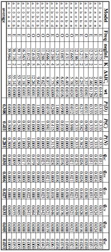
105 102

106 103 Table 3.2: Continuous character models. Discrete data (foraging time as a two-state (diurnal (D) / not diurnal (N) character was mapped on the tree using evolutionary pathway likelihood and the best-fitting model (non-reversible with equilibrium frequencies). Various continuous character models were then fitted to these trees. Not all models have all parameters; gray boxes represent parameters not in a given model.

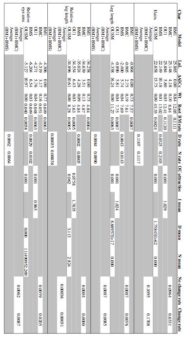
107 104