A Generative Perspective on MRFs in Low-Level Vision Supplemental Material
|
|
|
- Gary Fisher
- 5 years ago
- Views:
Transcription
1 A Generative Perspective on MRFs in Low-Level Vision Supplemental Material Uwe Schmidt Qi Gao Stefan Roth Department of Computer Science, TU Darmstadt 1. Derivations 1.1. Sampling the Prior We first rewrite the model density from Eqs. 1) and 2) of the main paper as px; Θ) = z 1 2 ZΘ) e ɛ x /2 c C N pz ic ) N J T i x c) ;, σi 2 /s zic ), 1) i=1 where we treat the scales z {1,..., J} N C for each expert and clique as random variables with pz ic ) = α izic i.e., the GSM mixture weights). Instead of marginalizing out the scales, we can also retain them explicitly and define the joint distribution cf. [13]) px, z; Θ) = 1 N 2 ZΘ) e ɛ x /2 pz ic ) N J T i x c) ;, σi 2 /s zic ). 2) c C i=1 The conditional distribution px z; Θ) can be derived as the multivariate Gaussian px z; Θ) e ɛ x 2 /2 c C 12 xt exp N i=1 N x;, ɛi + exp s ) z ic ) J T 2 2σi 2 i x c) ) ) N s zic σ 2 w ic wic T x i=1 c C i N ) ) 1 W i Z i Wi T, ɛi + i=1 where the w ic are defined such that w T ic x is the result of applying filter J i to clique c of the image x. Z i = diag{s zic /σ 2 i } are diagonal matrices with entries for each clique, and W i are filter matrices that correspond to a convolution of the image with filter J i, i.e. W T i x = [wt ic 1 x,..., w T ic C x] T = [J T i x C 1),..., J T i x C C )] T. Following Levi and Weiss [4, 11], we further rewrite the covariance as the matrix product Σ = ɛi + ) 1 N W i Z i Wi T = [W 1,..., W N, I] i=1 Z Z N ɛi W T 1. WN T I and sample y N, I) to obtain a sample x from px z; Θ) by solving the least-squares problem The first two authors contributed equally to this work. 1 = WZW T) 1 WZW T x = W Zy. 5) 3) 4) 1
2 By using the well-known property it follows that y N, I) Ay N, AIA T ), 6) x = WZW T) 1 WZW W Zy N T x;, ) 1 ) WZW W Z T I ) 1 ) ) T W Z N x;, WZW T) ) 7) 1 is indeed a valid sample from the conditional distribution as derived in Eq. 3). Since the scales are conditionally independent given the image by construction, the conditional distribution pz x; Θ) is readily given as 1.2. Conditional Sampling pz ic x; Θ) pz ic ) N J T i x c) ;, σ 2 i /s zic ). 8) In order to avoid extreme values at the less constrained boundary pixels [5] during learning and model analysis, or to perform inpainting of missing pixels given the known ones, we rely on conditional sampling. In particular, we sample the pixels x A given fixed x B and scales z according to the conditional Gaussian distribution px A x B, z; Θ), 9) where A and B denote the index sets of the respective pixels. Without loss of generality, we assume that x = [ xa x B ], Σ = WZW T) [ ] 1 1 A C = C T, 1) B where the square sub-matrix A has as many rows and columns as the vector x A has elements, etc. The conditional distribution of interest can now be derived as px A x B, z; Θ) exp 1 [ ] T [ ] [ ] ) xa A C xa 2 x B C T B x B exp 1 xa + A 1 ) T Cx B A xa + A 1 ) ) 11) Cx B 2 N x A ; A 1 Cx B, A 1). The matrices A and C are given by the appropriate sub-matrices of W i and Z i, and allow for the same efficient sampling scheme. The mean µ = A 1 Cx B can also be computed by solving a least squares problem. Sampling the conditional distribution of scales pz x A, x B ; Θ) = pz x; Θ) remains as before Sampling the Posterior for Image Denoising Assuming additive i. i. d. Gaussian noise with known standard derivation σ, the posterior given scales z can be written as px y, z; Θ) py x) px z; Θ) exp 1 2σ 2 y x 2) exp 1 ) 2 xt Σ 1 x exp 1 2x T y ) )) I 2 σ 2 + xt σ 2 + Σ 1 x N x; Σy/σ 2, Σ ), 12) where Σ = I/σ 2 + Σ 1) 1 and Σ as in Eq. 4). The conditional distribution of the scales pz x, y; Θ) = pz x; Θ) remains as before. 2
3 2. Image Restoration To further illustrate the image restoration performance of our approach, we provide the following additional results: Table 1 repeats Tab. 1 of the main paper and additionally gives the numerical results of MAP estimation with graph cuts and α-expansion [1]. Note that in most cases, α-expansion performs slightly worse in terms of PSNR than conjugate gradients, even and in fact particularly) for non-convex potentials. Also, using a Student-t potential [3] does not show favorable results. Table 2 shows the results of the same experiment as in Tab. 1, but reports the performance in terms of the perceptually more relevant structural similarity index SSIM) [1]. Note that all of the conclusions reported in the main paper also hold for this perceptual quality metric. Table 3 repeats Tab. 2 of the main paper, and additionally reports standard deviations as well as SSIM performance. The SSIM supports the same conclusions about relative performance as the PSNR. Figs. 1 6 show denoising results for 6 of the 68 images, for which the average performance is reported in Tab. 2 of the main paper. Note that in contrast to the tested previous approaches, combining our learned models with MMSE leads to good performance on relatively smooth as well as on strongly textured images. Fig. 7 provides a different view of the summary results in Tab. 2 of the paper. Instead of the average performance, we show a per-image comparison between the denoising results of the discriminative approach of [8] using MAP) and the results of our generatively-trained 3 3 FoE using MMSE). Note that the PSNR and particularly the SSIM show a substantial performance advantage for our approach. Fig. 8 shows an uncropped version of the inpainting result in Fig. 7 of the paper. Additionally, one other inpainting result is provided as further visual illustration. 3. Sampling the Prior and Posterior The following additional results illustrate properties of the auxiliary-variable Gibbs sampler. Fig. 9 shows five subsequent samples after reaching the equilibrium distribution) from all models listed in Table 1. Note how samples from common pairwise models appear too grainy, while those from previous FoE models are too smooth and without discontinuities. Fig. 1 shows two larger samples from our learned models. Note that our pairwise model leads to locally uniform samples with occasional discontinuities that appear spatially isolated speckles ). Our learned high-order model, on the other hand, leads to smoothly varying samples with occasional spatially correlated discontinuities, which appear more realistic. Fig. 11 illustrates the convergence of the sampling procedure for the prior and the posterior in case of denoising). Fig. 12 illustrates the advantages of running multiple parallel samplers. References [1] Y. Boykov, O. Veksler, and R. Zabih. Fast approximate energy minimization via graph cuts. PAMI, 2311): , 21. [2] A. Buades, B. Coll, and J.-M. Morel. A non-local algorithm for image denoising. CVPR 25. [3] X. Lan, S. Roth, D. P. Huttenlocher, and M. J. Black. Efficient belief propagation with learned higher-order Markov random fields. ECCV 26. [4] E. Levi. Using natural image priors Maximizing or sampling? Master s thesis, The Hebrew University of Jerusalem, 29. [5] M. Norouzi, M. Ranjbar, and G. Mori. Stacks of convolutional restricted Boltzmann machines for shift-invariant feature learning. CVPR, 29. [6] J. Portilla, V. Strela, M. J. Wainwright, and E. P. Simoncelli. Image denoising using scale mixtures of Gaussians in the wavelet domain. IEEE TIP, 1211): , 23. [7] S. Roth and M. J. Black. Fields of experts. IJCV, 822):25 229, 29. [8] K. G. G. Samuel and M. F. Tappen. Learning optimized MAP estimates in continuously-valued MRF models. CVPR 29. 3
4 Model MAP λ=1) MAP opt. λ) MMSE conj. gradient α-expansion conj. gradient α-expansion σ=1 σ=2 σ=1 σ=2 σ=1 σ=2 σ=1 σ=2 σ=1 σ=2 pairwise marginal fitting) pairwise generalized Laplacian [9]) pairwise Laplacian) pairwise Student-t [3]) pairwise ours) FoE from [7] FoE from [12] FoE ours) Table 1. Average PSNR db) of denoising results for 1 test images [3]. Model MAP λ=1) MAP opt. λ) MMSE conj. gradient α-expansion conj. gradient α-expansion σ=1 σ=2 σ=1 σ=2 σ=1 σ=2 σ=1 σ=2 σ=1 σ=2 pairwise marginal fitting) pairwise generalized Laplacian [9]) pairwise Laplacian) pairwise Student-t [3]) pairwise ours) FoE from [7] FoE from [12] FoE ours) Table 2. Average SSIM [1] of denoising results for 1 test images [3]. PSNR in db SSIM [1] Model Learning Inference average std. dev. average std. dev. 5 5 FoE from [7] CD generative) MAP w/λ FoE from [8] discriminative MAP pairwise ours) CD generative) MMSE FoE ours) CD generative) MMSE Non-local means [2] MMSE) BLS-GSM [6] MMSE Table 3. Denoising results for 68 test images [7, 8] σ = 25). [9] M. F. Tappen, B. C. Russell, and W. T. Freeman. Exploiting the sparse derivative prior for super-resolution and image demosaicing. Int. Workshop SCTV, 23. [1] Z. Wang, A. C. Bovik, H. R. Sheikh, and E. P. Simoncelli. Image quality assessment: From error visibility to structural similarity. IEEE TIP, 134):6 612, 24. [11] Y. Weiss. Personal communication, 25. [12] Y. Weiss and W. T. Freeman. What makes a good model of natural images? CVPR 27. [13] M. Welling, G. E. Hinton, and S. Osindero. Learning sparse topographic representations with products of Student-t distributions. NIPS*22. 4

 Pairwise g. Lapl.")
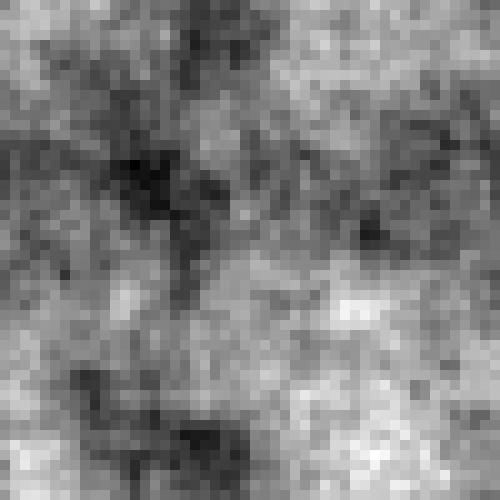
![[9]), PSNR = 27.65dB, SSIM =.](/docs-images/85/92787683/images/5-2.jpg "749 e) Pairwise ours), PSNR = 28.")
 3 3 FoE ours), PSNR = 28.")
 5 5 FoE from [7], PSNR = 28.")
 5 5 FoE from [8], PSNR = 28.")
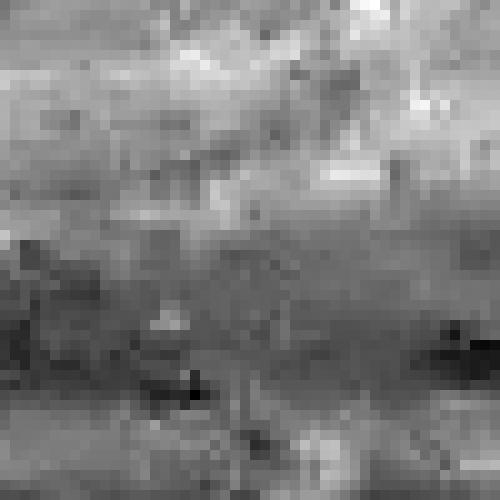
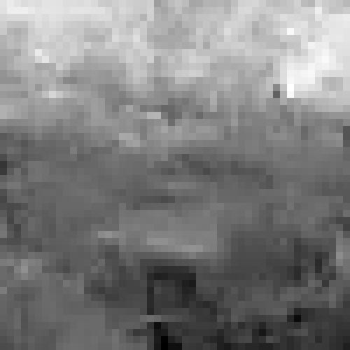
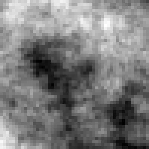
5 a) Original b) Noisy σ = 25), PSNR = 2.29dB, SSIM =.31 c) Pairwise Laplacian), PSNR = 27.88dB, SSIM =.763 d) Pairwise g. Lapl. [9]), PSNR = 27.65dB, SSIM =.749 e) Pairwise ours), PSNR = 28.34dB, SSIM =.779 f) 3 3 FoE ours), PSNR = 28.7dB, SSIM =.829 g) 5 5 FoE from [7], PSNR = 28.52dB, SSIM =.816 h) 5 5 FoE from [8], PSNR = 28.51dB, SSIM =.89 Figure 1. Denoising results for test image Castle : e, f) MMSE, c, d, g) MAP w/λ, h) MAP. 5

 Pairwise g. Lapl.")
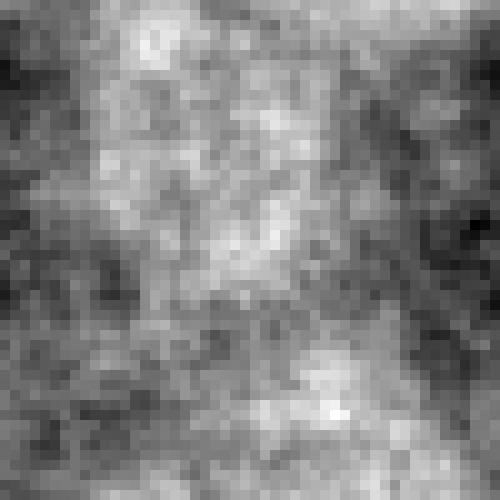
![[9]), PSNR = 27.87dB, SSIM =.](/docs-images/85/92787683/images/6-2.jpg "711 e) Pairwise ours), PSNR = 29.dB, SSIM =.")

![82 g) 5 5 FoE from [7], PSNR = 29.](/docs-images/85/92787683/images/6-4.jpg "16dB, SSIM =.")
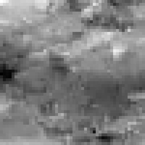
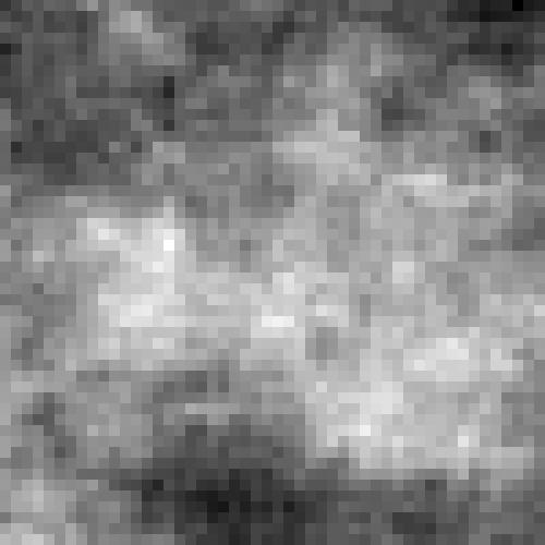
6 a) Original b) Noisy σ = 25), PSNR = 2.22dB, SSIM =.297 c) Pairwise Laplacian), PSNR = 28.78dB, SSIM =.757 d) Pairwise g. Lapl. [9]), PSNR = 27.87dB, SSIM =.711 e) Pairwise ours), PSNR = 29.dB, SSIM =.768 f) 3 3 FoE ours), PSNR = 29.79dB, SSIM =.82 g) 5 5 FoE from [7], PSNR = 29.16dB, SSIM =.794 h) 5 5 FoE from [8], PSNR = 29.35dB, SSIM =.82 Figure 2. Denoising results for test image Birds : e, f) MMSE, c, d, g) MAP w/λ, h) MAP. 6
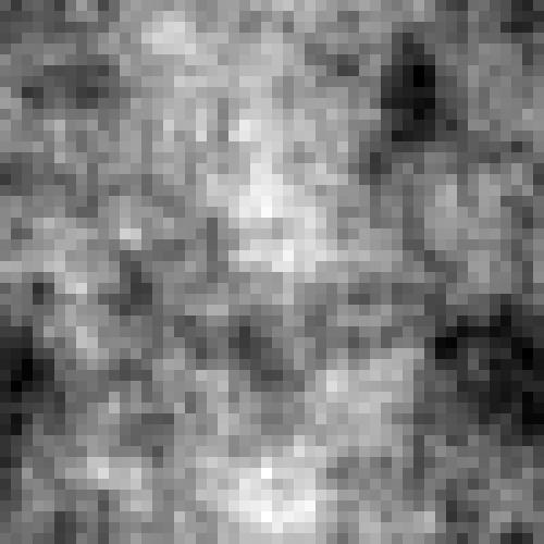
 Pairwise g. Lapl. [9]), PSNR = 26.12dB, SSIM =.781 e) Pairwise ours), PSNR = 26.51dB, SSIM =.")
![794 f) 3 3 FoE ours), PSNR = 27.dB, SSIM =.813 g) 5 5 FoE from [7], PSNR = 26.84dB, SSIM =.](/docs-images/85/92787683/images/7-1.jpg "792 h) 5 5 FoE from [8], PSNR = 27.6dB, SSIM =.817 Figure 3.")
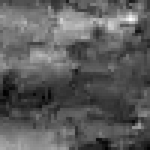
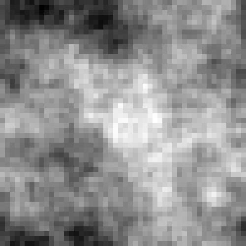
7 a) Original b) Noisy σ = 25), PSNR = 2.71dB, SSIM =.57 c) Pairwise Laplacian), PSNR = 26.32dB, SSIM =.789 d) Pairwise g. Lapl. [9]), PSNR = 26.12dB, SSIM =.781 e) Pairwise ours), PSNR = 26.51dB, SSIM =.794 f) 3 3 FoE ours), PSNR = 27.dB, SSIM =.813 g) 5 5 FoE from [7], PSNR = 26.84dB, SSIM =.792 h) 5 5 FoE from [8], PSNR = 27.6dB, SSIM =.817 Figure 3. Denoising results for test image LA : e, f) MMSE, c,d, g) MAP w/λ, h) MAP. 7
, PSNR = 2.34dB, SSIM =.")

, PSNR = 25.")
 Pairwise ours), PSNR")
 3 3 FoE ours), PSNR")
 5 5 FoE from [7],")
 5 5 FoE from [8],")

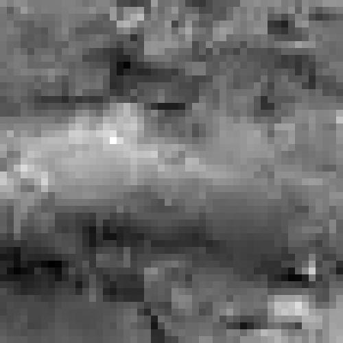
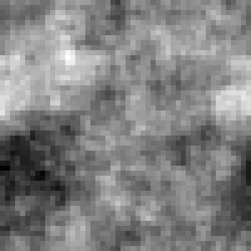
8 a) Original b) Noisy σ = 25), PSNR = 2.34dB, SSIM =.475 c) Pairwise Laplacian), PSNR = 25.93dB, SSIM =.674 d) Pairwise g. Lapl. [9]), PSNR = 25.36dB, SSIM =.647 e) Pairwise ours), PSNR = 26.12dB, SSIM =.685 f) 3 3 FoE ours), PSNR = 26.27dB, SSIM =.689 g) 5 5 FoE from [7], PSNR = 25.36dB, SSIM =.592 h) 5 5 FoE from [8], PSNR = 26.19dB, SSIM =.686 Figure 4. Denoising results for test image Goat : e, f) MMSE, c, d, g) MAP w/λ, h) MAP. 8
![a) Original b) Noisy σ = 25), PSNR = 22.44dB, SSIM =.278 c) Pairwise Laplacian), PSNR = 28.77dB, SSIM =.838 d) Pairwise g. Lapl. [9]), PSNR = 28.65dB, SSIM =.831 e) Pairwise ours), PSNR = 28.](/docs-images/85/92787683/images/9-0.jpg "81dB, SSIM =.829 f) 3 3 FoE ours), PSNR = 28.72dB, SSIM =.834 g) 5 5 FoE from [7], PSNR = 28.52dB, SSIM =.82 h) 5 5 FoE from [8], PSNR = 3.99dB, SSIM =.81 Figure 5.")
9 a) Original b) Noisy σ = 25), PSNR = 22.44dB, SSIM =.278 c) Pairwise Laplacian), PSNR = 28.77dB, SSIM =.838 d) Pairwise g. Lapl. [9]), PSNR = 28.65dB, SSIM =.831 e) Pairwise ours), PSNR = 28.81dB, SSIM =.829 f) 3 3 FoE ours), PSNR = 28.72dB, SSIM =.834 g) 5 5 FoE from [7], PSNR = 28.52dB, SSIM =.82 h) 5 5 FoE from [8], PSNR = 3.99dB, SSIM =.81 Figure 5. Denoising results for test image Wolf : e, f) MMSE, c, d, g) MAP w/λ, h) MAP. 9
, PSNR = 2.21dB, SSIM =.")

, PSNR = 32.")
 Pairwise ours), PSNR")
 3 3 FoE ours), PSNR")
 5 5 FoE from [7],")
 5 5 FoE from [8],")

10 a) Original b) Noisy σ = 25), PSNR = 2.21dB, SSIM =.136 c) Pairwise Laplacian), PSNR = 32.78dB, SSIM =.89 d) Pairwise g. Lapl. [9]), PSNR = 32.36dB, SSIM =.87 e) Pairwise ours), PSNR = 33.51dB, SSIM =.829 f) 3 3 FoE ours), PSNR = 35.28dB, SSIM =.931 g) 5 5 FoE from [7], PSNR = 35.dB, SSIM =.938 h) 5 5 FoE from [8], PSNR = 33.63dB, SSIM =.881 Figure 6. Denoising results for test image Airplane : e, f) MMSE, c, d, g) MAP w/λ, h) MAP. 1
 using FoE of Samuel and Tappen a).5 Ours better Samuel and Tappen better.5.6.7.8.9 SSIM using FoE of Samuel and Tappen b) Figure 7.")
![Comparing the denoising performance σ = 25) in terms of a) PSNR and b) SSIM for 68 test images between our 3 3 FoE using MMSE) and the 5 5 FoE from [8] using MAP).](/docs-images/85/92787683/images/11-1.jpg "A red circle above the black line means performance is better with our approach. a) Original photograph b) Restored with our pairwise MRF c) Original photograph Figure 8.")
11 PSNR db) using our 3x3 FoE Airplane Wolf SSIM using our 3x3 FoE Ours better Samuel and Tappen better PSNR db) using FoE of Samuel and Tappen a).5 Ours better Samuel and Tappen better SSIM using FoE of Samuel and Tappen b) Figure 7. Comparing the denoising performance σ = 25) in terms of a) PSNR and b) SSIM for 68 test images between our 3 3 FoE using MMSE) and the 5 5 FoE from [8] using MAP). A red circle above the black line means performance is better with our approach. a) Original photograph b) Restored with our pairwise MRF c) Original photograph Figure 8. MMSE-based image inpainting with our learned models. d) Restored with our 3 3 FoE 11
")


 3 3")


 15")
12 a) Pairwise, ours b) Pairwise, marginal fitting c) Pairwise, generalized Laplacian from [9] d) Pairwise, Laplacian e) 3 3 FoE, ours f) 5 5 FoE from [7] x g) FoE from [12] convolution with circular boundary handling, no pixels removed) Figure 9. Five subsequent samples l. to r.) from various MRF models after reaching the equilibrium distribution. The boundary pixels are removed for better visualization x
 Prior 3.")
.")
13 a) Pairwise MRF 5 b) 3 3 FoE Figure pixel sample from our learned models after reaching the equilibrium distribution. The boundary pixels are removed for better visualization. 15 energy 2.6 x energy 4.6 x # of iterations a) Prior # of iterations b) Posterior Figure 11. Monitoring the convergence of sampling. a) Sampling a 5 5 image from the learned pairwise MRF prior conditioned on a 1-pixel boundary. Three chains and over-dispersed starting points red, dashed interior of the boundary image; blue, solid medianfiltered version; black, dash-dotted noisy version). Approximate convergence is reached after 25 iterations ˆR < 1.1). b) Sampling the posterior σ = 2, image size 16 24) with four chains and over-dispersed starting points red, dashed noisy image; blue, dash-dotted Gauss filtered version; green, solid median filtered version; black, dotted Wiener filtered version). Approximate convergence is reached after 24 iterations PSNR PSNR samplers 4 samplers 26 2 samplers 1 sampler # of iterations a) Assuming parallel computing 26 1 samplers 4 samplers 2 samplers 1 sampler # of samples b) Assuming sequential computing Figure 12. Efficiency of sampling-based MMSE denoising with different number of samplers. Learned pairwise MRF, σ = 2, image size a) In case of parallel computing one sampler per computing core), faster convergence of the denoised image can be achieved. b) Even when using sequential computing, multiple samplers can improve performance, as the samples are less correlated. 13
Modeling Natural Images with Higher-Order Boltzmann Machines
 Modeling Natural Images with Higher-Order Boltzmann Machines Marc'Aurelio Ranzato Department of Computer Science Univ. of Toronto ranzato@cs.toronto.edu joint work with Geoffrey Hinton and Vlad Mnih CIFAR
Image representation with multi-scale gradients
 Image representation with multi-scale gradients Eero P Simoncelli Center for Neural Science, and Courant Institute of Mathematical Sciences New York University http://www.cns.nyu.edu/~eero Visual image
Discriminative Fields for Modeling Spatial Dependencies in Natural Images
 Discriminative Fields for Modeling Spatial Dependencies in Natural Images Sanjiv Kumar and Martial Hebert The Robotics Institute Carnegie Mellon University Pittsburgh, PA 15213 {skumar,hebert}@ri.cmu.edu
Markov Random Fields
 Markov Random Fields Umamahesh Srinivas ipal Group Meeting February 25, 2011 Outline 1 Basic graph-theoretic concepts 2 Markov chain 3 Markov random field (MRF) 4 Gauss-Markov random field (GMRF), and
TUTORIAL PART 1 Unsupervised Learning
 TUTORIAL PART 1 Unsupervised Learning Marc'Aurelio Ranzato Department of Computer Science Univ. of Toronto ranzato@cs.toronto.edu Co-organizers: Honglak Lee, Yoshua Bengio, Geoff Hinton, Yann LeCun, Andrew
Linear Dynamical Systems
 Linear Dynamical Systems Sargur N. srihari@cedar.buffalo.edu Machine Learning Course: http://www.cedar.buffalo.edu/~srihari/cse574/index.html Two Models Described by Same Graph Latent variables Observations
Contrastive Divergence
 Contrastive Divergence Training Products of Experts by Minimizing CD Hinton, 2002 Helmut Puhr Institute for Theoretical Computer Science TU Graz June 9, 2010 Contents 1 Theory 2 Argument 3 Contrastive
Hierarchical Sparse Bayesian Learning. Pierre Garrigues UC Berkeley
 Hierarchical Sparse Bayesian Learning Pierre Garrigues UC Berkeley Outline Motivation Description of the model Inference Learning Results Motivation Assumption: sensory systems are adapted to the statistical
Unsupervised Learning of Hierarchical Models. in collaboration with Josh Susskind and Vlad Mnih
 Unsupervised Learning of Hierarchical Models Marc'Aurelio Ranzato Geoff Hinton in collaboration with Josh Susskind and Vlad Mnih Advanced Machine Learning, 9 March 2011 Example: facial expression recognition
Variational Inference (11/04/13)
") STA561: Probabilistic machine learning Variational Inference (11/04/13) Lecturer: Barbara Engelhardt Scribes: Matt Dickenson, Alireza Samany, Tracy Schifeling 1 Introduction In this lecture we will further
STA561: Probabilistic machine learning Variational Inference (11/04/13) Lecturer: Barbara Engelhardt Scribes: Matt Dickenson, Alireza Samany, Tracy Schifeling 1 Introduction In this lecture we will further
Probabilistic Graphical Models
 2016 Robert Nowak Probabilistic Graphical Models 1 Introduction We have focused mainly on linear models for signals, in particular the subspace model x = Uθ, where U is a n k matrix and θ R k is a vector
Undirected Graphical Models: Markov Random Fields
 Undirected Graphical Models: Markov Random Fields 40-956 Advanced Topics in AI: Probabilistic Graphical Models Sharif University of Technology Soleymani Spring 2015 Markov Random Field Structure: undirected
Efficient Variational Inference in Large-Scale Bayesian Compressed Sensing
 Efficient Variational Inference in Large-Scale Bayesian Compressed Sensing George Papandreou and Alan Yuille Department of Statistics University of California, Los Angeles ICCV Workshop on Information
Image Denoising using Uniform Curvelet Transform and Complex Gaussian Scale Mixture
 EE 5359 Multimedia Processing Project Report Image Denoising using Uniform Curvelet Transform and Complex Gaussian Scale Mixture By An Vo ISTRUCTOR: Dr. K. R. Rao Summer 008 Image Denoising using Uniform
Bayesian Learning in Undirected Graphical Models
 Bayesian Learning in Undirected Graphical Models Zoubin Ghahramani Gatsby Computational Neuroscience Unit University College London, UK http://www.gatsby.ucl.ac.uk/ Work with: Iain Murray and Hyun-Chul
A Graph Cut Algorithm for Generalized Image Deconvolution
 A Graph Cut Algorithm for Generalized Image Deconvolution Ashish Raj UC San Francisco San Francisco, CA 94143 Ramin Zabih Cornell University Ithaca, NY 14853 Abstract The goal of deconvolution is to recover
PILCO: A Model-Based and Data-Efficient Approach to Policy Search
 PILCO: A Model-Based and Data-Efficient Approach to Policy Search (M.P. Deisenroth and C.E. Rasmussen) CSC2541 November 4, 2016 PILCO Graphical Model PILCO Probabilistic Inference for Learning COntrol
A Graph Cut Algorithm for Higher-order Markov Random Fields
 A Graph Cut Algorithm for Higher-order Markov Random Fields Alexander Fix Cornell University Aritanan Gruber Rutgers University Endre Boros Rutgers University Ramin Zabih Cornell University Abstract Higher-order
Markov Random Fields for Computer Vision (Part 1)
") Markov Random Fields for Computer Vision (Part 1) Machine Learning Summer School (MLSS 2011) Stephen Gould stephen.gould@anu.edu.au Australian National University 13 17 June, 2011 Stephen Gould 1/23 Pixel
Markov Random Fields for Computer Vision (Part 1) Machine Learning Summer School (MLSS 2011) Stephen Gould stephen.gould@anu.edu.au Australian National University 13 17 June, 2011 Stephen Gould 1/23 Pixel
Introduction to Machine Learning
 Introduction to Machine Learning Brown University CSCI 1950-F, Spring 2012 Prof. Erik Sudderth Lecture 25: Markov Chain Monte Carlo (MCMC) Course Review and Advanced Topics Many figures courtesy Kevin
Intelligent Systems:
 Intelligent Systems: Undirected Graphical models (Factor Graphs) (2 lectures) Carsten Rother 15/01/2015 Intelligent Systems: Probabilistic Inference in DGM and UGM Roadmap for next two lectures Definition
Probabilistic Graphical Models Lecture Notes Fall 2009
 Probabilistic Graphical Models Lecture Notes Fall 2009 October 28, 2009 Byoung-Tak Zhang School of omputer Science and Engineering & ognitive Science, Brain Science, and Bioinformatics Seoul National University
Approximate Inference Part 1 of 2
 Approximate Inference Part 1 of 2 Tom Minka Microsoft Research, Cambridge, UK Machine Learning Summer School 2009 http://mlg.eng.cam.ac.uk/mlss09/ Bayesian paradigm Consistent use of probability theory
Approximate Inference Part 1 of 2
 Approximate Inference Part 1 of 2 Tom Minka Microsoft Research, Cambridge, UK Machine Learning Summer School 2009 http://mlg.eng.cam.ac.uk/mlss09/ 1 Bayesian paradigm Consistent use of probability theory
Poisson Image Denoising Using Best Linear Prediction: A Post-processing Framework
 Poisson Image Denoising Using Best Linear Prediction: A Post-processing Framework Milad Niknejad, Mário A.T. Figueiredo Instituto de Telecomunicações, and Instituto Superior Técnico, Universidade de Lisboa,
Noise-Blind Image Deblurring Supplementary Material
 Noise-Blind Image Deblurring Supplementary Material Meiguang Jin University of Bern Switzerland Stefan Roth TU Darmstadt Germany Paolo Favaro University of Bern Switzerland A. Upper and Lower Bounds Our
CPSC 540: Machine Learning
 CPSC 540: Machine Learning Undirected Graphical Models Mark Schmidt University of British Columbia Winter 2016 Admin Assignment 3: 2 late days to hand it in today, Thursday is final day. Assignment 4:
Pattern Recognition and Machine Learning
 Christopher M. Bishop Pattern Recognition and Machine Learning ÖSpri inger Contents Preface Mathematical notation Contents vii xi xiii 1 Introduction 1 1.1 Example: Polynomial Curve Fitting 4 1.2 Probability
Restricted Boltzmann Machines for Collaborative Filtering
 Restricted Boltzmann Machines for Collaborative Filtering Authors: Ruslan Salakhutdinov Andriy Mnih Geoffrey Hinton Benjamin Schwehn Presentation by: Ioan Stanculescu 1 Overview The Netflix prize problem
Lecture 16 Deep Neural Generative Models
 Lecture 16 Deep Neural Generative Models CMSC 35246: Deep Learning Shubhendu Trivedi & Risi Kondor University of Chicago May 22, 2017 Approach so far: We have considered simple models and then constructed
What makes a good model of natural images?
 0 0.5.5.5 3 dx.8.6.4. 0.8 0.6 0.4 0. 0 40 30 0 0 0 0 0 30 40 G*dx 9 8 7 6 5 4 3 0 40 30 0 0 0 0 0 30 40 G*G*G*dx What maes a good model of natural images? Yair Weiss, Hebrew University of Jerusalem yweiss@cs.huji.ac.il
Probabilistic Graphical Models
 Probabilistic Graphical Models Brown University CSCI 295-P, Spring 213 Prof. Erik Sudderth Lecture 11: Inference & Learning Overview, Gaussian Graphical Models Some figures courtesy Michael Jordan s draft
Linear Dynamical Systems (Kalman filter)
") Linear Dynamical Systems (Kalman filter) (a) Overview of HMMs (b) From HMMs to Linear Dynamical Systems (LDS) 1 Markov Chains with Discrete Random Variables x 1 x 2 x 3 x T Let s assume we have discrete
Linear Dynamical Systems (Kalman filter) (a) Overview of HMMs (b) From HMMs to Linear Dynamical Systems (LDS) 1 Markov Chains with Discrete Random Variables x 1 x 2 x 3 x T Let s assume we have discrete
Higher-Order Clique Reduction in Binary Graph Cut
 CVPR009: IEEE Computer Society Conference on Computer Vision and Pattern Recognition, Miami Beach, Florida. June 0-5, 009. Hiroshi Ishikawa Nagoya City University Department of Information and Biological
Chapter 16. Structured Probabilistic Models for Deep Learning
 Peng et al.: Deep Learning and Practice 1 Chapter 16 Structured Probabilistic Models for Deep Learning Peng et al.: Deep Learning and Practice 2 Structured Probabilistic Models way of using graphs to describe
Bayesian Image Segmentation Using MRF s Combined with Hierarchical Prior Models
 Bayesian Image Segmentation Using MRF s Combined with Hierarchical Prior Models Kohta Aoki 1 and Hiroshi Nagahashi 2 1 Interdisciplinary Graduate School of Science and Engineering, Tokyo Institute of Technology
Higher-Order Clique Reduction Without Auxiliary Variables
 Higher-Order Clique Reduction Without Auxiliary Variables Hiroshi Ishikawa Department of Computer Science and Engineering Waseda University Okubo 3-4-1, Shinjuku, Tokyo, Japan hfs@waseda.jp Abstract We
Undirected Graphical Models
 Outline Hong Chang Institute of Computing Technology, Chinese Academy of Sciences Machine Learning Methods (Fall 2012) Outline Outline I 1 Introduction 2 Properties Properties 3 Generative vs. Conditional
CPSC 540: Machine Learning
 CPSC 540: Machine Learning MCMC and Non-Parametric Bayes Mark Schmidt University of British Columbia Winter 2016 Admin I went through project proposals: Some of you got a message on Piazza. No news is
Chris Bishop s PRML Ch. 8: Graphical Models
 Chris Bishop s PRML Ch. 8: Graphical Models January 24, 2008 Introduction Visualize the structure of a probabilistic model Design and motivate new models Insights into the model s properties, in particular
Alternative Parameterizations of Markov Networks. Sargur Srihari
 Alternative Parameterizations of Markov Networks Sargur srihari@cedar.buffalo.edu 1 Topics Three types of parameterization 1. Gibbs Parameterization 2. Factor Graphs 3. Log-linear Models with Energy functions
Low-Complexity Image Denoising via Analytical Form of Generalized Gaussian Random Vectors in AWGN
 Low-Complexity Image Denoising via Analytical Form of Generalized Gaussian Random Vectors in AWGN PICHID KITTISUWAN Rajamangala University of Technology (Ratanakosin), Department of Telecommunication Engineering,
Introduction to Nonlinear Image Processing
 Introduction to Nonlinear Image Processing 1 IPAM Summer School on Computer Vision July 22, 2013 Iasonas Kokkinos Center for Visual Computing Ecole Centrale Paris / INRIA Saclay Mean and median 2 Observations
STA 4273H: Statistical Machine Learning
 STA 4273H: Statistical Machine Learning Russ Salakhutdinov Department of Statistics! rsalakhu@utstat.toronto.edu! http://www.utstat.utoronto.ca/~rsalakhu/ Sidney Smith Hall, Room 6002 Lecture 3 Linear
The Origin of Deep Learning. Lili Mou Jan, 2015
 The Origin of Deep Learning Lili Mou Jan, 2015 Acknowledgment Most of the materials come from G. E. Hinton s online course. Outline Introduction Preliminary Boltzmann Machines and RBMs Deep Belief Nets
Gaussian Processes for Audio Feature Extraction
 Gaussian Processes for Audio Feature Extraction Dr. Richard E. Turner (ret26@cam.ac.uk) Computational and Biological Learning Lab Department of Engineering University of Cambridge Machine hearing pipeline
CSC 412 (Lecture 4): Undirected Graphical Models
: Undirected Graphical Models") CSC 412 (Lecture 4): Undirected Graphical Models Raquel Urtasun University of Toronto Feb 2, 2016 R Urtasun (UofT) CSC 412 Feb 2, 2016 1 / 37 Today Undirected Graphical Models: Semantics of the graph:
CSC 412 (Lecture 4): Undirected Graphical Models Raquel Urtasun University of Toronto Feb 2, 2016 R Urtasun (UofT) CSC 412 Feb 2, 2016 1 / 37 Today Undirected Graphical Models: Semantics of the graph:
Over-enhancement Reduction in Local Histogram Equalization using its Degrees of Freedom. Alireza Avanaki
 Over-enhancement Reduction in Local Histogram Equalization using its Degrees of Freedom Alireza Avanaki ABSTRACT A well-known issue of local (adaptive) histogram equalization (LHE) is over-enhancement
Better restore the recto side of a document with an estimation of the verso side: Markov model and inference with graph cuts
 June 23 rd 2008 Better restore the recto side of a document with an estimation of the verso side: Markov model and inference with graph cuts Christian Wolf Laboratoire d InfoRmatique en Image et Systèmes
Does Better Inference mean Better Learning?
 Does Better Inference mean Better Learning? Andrew E. Gelfand, Rina Dechter & Alexander Ihler Department of Computer Science University of California, Irvine {agelfand,dechter,ihler}@ics.uci.edu Abstract
Learning Energy-Based Models of High-Dimensional Data
 Learning Energy-Based Models of High-Dimensional Data Geoffrey Hinton Max Welling Yee-Whye Teh Simon Osindero www.cs.toronto.edu/~hinton/energybasedmodelsweb.htm Discovering causal structure as a goal
Deep Learning Srihari. Deep Belief Nets. Sargur N. Srihari
 Deep Belief Nets Sargur N. Srihari srihari@cedar.buffalo.edu Topics 1. Boltzmann machines 2. Restricted Boltzmann machines 3. Deep Belief Networks 4. Deep Boltzmann machines 5. Boltzmann machines for continuous
A graph contains a set of nodes (vertices) connected by links (edges or arcs)
 connected by links (edges or arcs)") BOLTZMANN MACHINES Generative Models Graphical Models A graph contains a set of nodes (vertices) connected by links (edges or arcs) In a probabilistic graphical model, each node represents a random variable,
BOLTZMANN MACHINES Generative Models Graphical Models A graph contains a set of nodes (vertices) connected by links (edges or arcs) In a probabilistic graphical model, each node represents a random variable,
Probabilistic Graphical Models
 Probabilistic Graphical Models Lecture 11 CRFs, Exponential Family CS/CNS/EE 155 Andreas Krause Announcements Homework 2 due today Project milestones due next Monday (Nov 9) About half the work should
Bayesian Machine Learning - Lecture 7
 Bayesian Machine Learning - Lecture 7 Guido Sanguinetti Institute for Adaptive and Neural Computation School of Informatics University of Edinburgh gsanguin@inf.ed.ac.uk March 4, 2015 Today s lecture 1
Density Propagation for Continuous Temporal Chains Generative and Discriminative Models
 $ Technical Report, University of Toronto, CSRG-501, October 2004 Density Propagation for Continuous Temporal Chains Generative and Discriminative Models Cristian Sminchisescu and Allan Jepson Department
Sequence labeling. Taking collective a set of interrelated instances x 1,, x T and jointly labeling them
 HMM, MEMM and CRF 40-957 Special opics in Artificial Intelligence: Probabilistic Graphical Models Sharif University of echnology Soleymani Spring 2014 Sequence labeling aking collective a set of interrelated
Generalized Roof Duality for Pseudo-Boolean Optimization
 Generalized Roof Duality for Pseudo-Boolean Optimization Fredrik Kahl Petter Strandmark Centre for Mathematical Sciences, Lund University, Sweden {fredrik,petter}@maths.lth.se Abstract The number of applications
Simultaneous Multi-frame MAP Super-Resolution Video Enhancement using Spatio-temporal Priors
 Simultaneous Multi-frame MAP Super-Resolution Video Enhancement using Spatio-temporal Priors Sean Borman and Robert L. Stevenson Department of Electrical Engineering, University of Notre Dame Notre Dame,
Efficient Inference in Fully Connected CRFs with Gaussian Edge Potentials
 Efficient Inference in Fully Connected CRFs with Gaussian Edge Potentials by Phillip Krahenbuhl and Vladlen Koltun Presented by Adam Stambler Multi-class image segmentation Assign a class label to each
Connections between score matching, contrastive divergence, and pseudolikelihood for continuous-valued variables. Revised submission to IEEE TNN
 Connections between score matching, contrastive divergence, and pseudolikelihood for continuous-valued variables Revised submission to IEEE TNN Aapo Hyvärinen Dept of Computer Science and HIIT University
Graphical Models and Kernel Methods
 Graphical Models and Kernel Methods Jerry Zhu Department of Computer Sciences University of Wisconsin Madison, USA MLSS June 17, 2014 1 / 123 Outline Graphical Models Probabilistic Inference Directed vs.
Graphical Models for Collaborative Filtering
 Graphical Models for Collaborative Filtering Le Song Machine Learning II: Advanced Topics CSE 8803ML, Spring 2012 Sequence modeling HMM, Kalman Filter, etc.: Similarity: the same graphical model topology,
Learning Gaussian Process Models from Uncertain Data
 Learning Gaussian Process Models from Uncertain Data Patrick Dallaire, Camille Besse, and Brahim Chaib-draa DAMAS Laboratory, Computer Science & Software Engineering Department, Laval University, Canada
Introduction to Machine Learning
 Introduction to Machine Learning Brown University CSCI 1950-F, Spring 2012 Prof. Erik Sudderth Lecture 20: Expectation Maximization Algorithm EM for Mixture Models Many figures courtesy Kevin Murphy s
Energy Based Models. Stefano Ermon, Aditya Grover. Stanford University. Lecture 13
 Energy Based Models Stefano Ermon, Aditya Grover Stanford University Lecture 13 Stefano Ermon, Aditya Grover (AI Lab) Deep Generative Models Lecture 13 1 / 21 Summary Story so far Representation: Latent
Is early vision optimised for extracting higher order dependencies? Karklin and Lewicki, NIPS 2005
 Is early vision optimised for extracting higher order dependencies? Karklin and Lewicki, NIPS 2005 Richard Turner (turner@gatsby.ucl.ac.uk) Gatsby Computational Neuroscience Unit, 02/03/2006 Outline Historical
Higher-order Graph Cuts
 ACCV2014 Area Chairs Workshop Sep. 3, 2014 Nanyang Technological University, Singapore 1 Higher-order Graph Cuts Hiroshi Ishikawa Department of Computer Science & Engineering Waseda University Labeling
Statistics 352: Spatial statistics. Jonathan Taylor. Department of Statistics. Models for discrete data. Stanford University.
 352: 352: Models for discrete data April 28, 2009 1 / 33 Models for discrete data 352: Outline Dependent discrete data. Image data (binary). Ising models. Simulation: Gibbs sampling. Denoising. 2 / 33
Human Pose Tracking I: Basics. David Fleet University of Toronto
 Human Pose Tracking I: Basics David Fleet University of Toronto CIFAR Summer School, 2009 Looking at People Challenges: Complex pose / motion People have many degrees of freedom, comprising an articulated
Message-Passing Algorithms for GMRFs and Non-Linear Optimization
 Message-Passing Algorithms for GMRFs and Non-Linear Optimization Jason Johnson Joint Work with Dmitry Malioutov, Venkat Chandrasekaran and Alan Willsky Stochastic Systems Group, MIT NIPS Workshop: Approximate
Introduction to Restricted Boltzmann Machines
 Introduction to Restricted Boltzmann Machines Ilija Bogunovic and Edo Collins EPFL {ilija.bogunovic,edo.collins}@epfl.ch October 13, 2014 Introduction Ingredients: 1. Probabilistic graphical models (undirected,
1 EM algorithm: updating the mixing proportions {π k } ik are the posterior probabilities at the qth iteration of EM.
 Université du Sud Toulon - Var Master Informatique Probabilistic Learning and Data Analysis TD: Model-based clustering by Faicel CHAMROUKHI Solution The aim of this practical wor is to show how the Classification
Cheng Soon Ong & Christian Walder. Canberra February June 2018
 Cheng Soon Ong & Christian Walder Research Group and College of Engineering and Computer Science Canberra February June 2018 Outlines Overview Introduction Linear Algebra Probability Linear Regression
Part 1: Expectation Propagation
 Chalmers Machine Learning Summer School Approximate message passing and biomedicine Part 1: Expectation Propagation Tom Heskes Machine Learning Group, Institute for Computing and Information Sciences Radboud
Deep Learning of Invariant Spatiotemporal Features from Video. Bo Chen, Jo-Anne Ting, Ben Marlin, Nando de Freitas University of British Columbia
 Deep Learning of Invariant Spatiotemporal Features from Video Bo Chen, Jo-Anne Ting, Ben Marlin, Nando de Freitas University of British Columbia Introduction Focus: Unsupervised feature extraction from
A NO-REFERENCE SHARPNESS METRIC SENSITIVE TO BLUR AND NOISE. Xiang Zhu and Peyman Milanfar
 A NO-REFERENCE SARPNESS METRIC SENSITIVE TO BLUR AND NOISE Xiang Zhu and Peyman Milanfar Electrical Engineering Department University of California at Santa Cruz, CA, 9564 xzhu@soeucscedu ABSTRACT A no-reference
MACHINE LEARNING 2 UGM,HMMS Lecture 7
 LOREM I P S U M Royal Institute of Technology MACHINE LEARNING 2 UGM,HMMS Lecture 7 THIS LECTURE DGM semantics UGM De-noising HMMs Applications (interesting probabilities) DP for generation probability
Lecture 9: PGM Learning
 13 Oct 2014 Intro. to Stats. Machine Learning COMP SCI 4401/7401 Table of Contents I Learning parameters in MRFs 1 Learning parameters in MRFs Inference and Learning Given parameters (of potentials) and
Computer Vision Group Prof. Daniel Cremers. 10a. Markov Chain Monte Carlo
 Group Prof. Daniel Cremers 10a. Markov Chain Monte Carlo Markov Chain Monte Carlo In high-dimensional spaces, rejection sampling and importance sampling are very inefficient An alternative is Markov Chain
Deep unsupervised learning
 Deep unsupervised learning Advanced data-mining Yongdai Kim Department of Statistics, Seoul National University, South Korea Unsupervised learning In machine learning, there are 3 kinds of learning paradigm.
Course 16:198:520: Introduction To Artificial Intelligence Lecture 9. Markov Networks. Abdeslam Boularias. Monday, October 14, 2015
 Course 16:198:520: Introduction To Artificial Intelligence Lecture 9 Markov Networks Abdeslam Boularias Monday, October 14, 2015 1 / 58 Overview Bayesian networks, presented in the previous lecture, are
Image Noise: Detection, Measurement and Removal Techniques. Zhifei Zhang
 Image Noise: Detection, Measurement and Removal Techniques Zhifei Zhang Outline Noise measurement Filter-based Block-based Wavelet-based Noise removal Spatial domain Transform domain Non-local methods
ARestricted Boltzmann machine (RBM) [1] is a probabilistic
![ARestricted Boltzmann machine (RBM) [1] is a probabilistic](/thumbs/90/102816372.jpg "ARestricted Boltzmann machine (RBM) [1] is a probabilistic") 1 Matrix Product Operator Restricted Boltzmann Machines Cong Chen, Kim Batselier, Ching-Yun Ko, and Ngai Wong chencong@eee.hku.hk, k.batselier@tudelft.nl, cyko@eee.hku.hk, nwong@eee.hku.hk arxiv:1811.04608v1
1 Matrix Product Operator Restricted Boltzmann Machines Cong Chen, Kim Batselier, Ching-Yun Ko, and Ngai Wong chencong@eee.hku.hk, k.batselier@tudelft.nl, cyko@eee.hku.hk, nwong@eee.hku.hk arxiv:1811.04608v1
Approximate Message Passing
 Approximate Message Passing Mohammad Emtiyaz Khan CS, UBC February 8, 2012 Abstract In this note, I summarize Sections 5.1 and 5.2 of Arian Maleki s PhD thesis. 1 Notation We denote scalars by small letters
Nonparametric Bayesian Methods (Gaussian Processes)
") [70240413 Statistical Machine Learning, Spring, 2015] Nonparametric Bayesian Methods (Gaussian Processes) Jun Zhu dcszj@mail.tsinghua.edu.cn http://bigml.cs.tsinghua.edu.cn/~jun State Key Lab of Intelligent
[70240413 Statistical Machine Learning, Spring, 2015] Nonparametric Bayesian Methods (Gaussian Processes) Jun Zhu dcszj@mail.tsinghua.edu.cn http://bigml.cs.tsinghua.edu.cn/~jun State Key Lab of Intelligent
Introduction to Probabilistic Graphical Models: Exercises
 Introduction to Probabilistic Graphical Models: Exercises Cédric Archambeau Xerox Research Centre Europe cedric.archambeau@xrce.xerox.com Pascal Bootcamp Marseille, France, July 2010 Exercise 1: basics
1 Bayesian Linear Regression (BLR)
") Statistical Techniques in Robotics (STR, S15) Lecture#10 (Wednesday, February 11) Lecturer: Byron Boots Gaussian Properties, Bayesian Linear Regression 1 Bayesian Linear Regression (BLR) In linear regression,
Statistical Techniques in Robotics (STR, S15) Lecture#10 (Wednesday, February 11) Lecturer: Byron Boots Gaussian Properties, Bayesian Linear Regression 1 Bayesian Linear Regression (BLR) In linear regression,
Expectation propagation for signal detection in flat-fading channels
 Expectation propagation for signal detection in flat-fading channels Yuan Qi MIT Media Lab Cambridge, MA, 02139 USA yuanqi@media.mit.edu Thomas Minka CMU Statistics Department Pittsburgh, PA 15213 USA
Alternative Parameterizations of Markov Networks. Sargur Srihari
 Alternative Parameterizations of Markov Networks Sargur srihari@cedar.buffalo.edu 1 Topics Three types of parameterization 1. Gibbs Parameterization 2. Factor Graphs 3. Log-linear Models Features (Ising,
Based on slides by Richard Zemel
 CSC 412/2506 Winter 2018 Probabilistic Learning and Reasoning Lecture 3: Directed Graphical Models and Latent Variables Based on slides by Richard Zemel Learning outcomes What aspects of a model can we
Unsupervised Learning
 Unsupervised Learning Bayesian Model Comparison Zoubin Ghahramani zoubin@gatsby.ucl.ac.uk Gatsby Computational Neuroscience Unit, and MSc in Intelligent Systems, Dept Computer Science University College
Undirected graphical models
 Undirected graphical models Semantics of probabilistic models over undirected graphs Parameters of undirected models Example applications COMP-652 and ECSE-608, February 16, 2017 1 Undirected graphical
A Unified Energy-Based Framework for Unsupervised Learning
 A Unified Energy-Based Framework for Unsupervised Learning Marc Aurelio Ranzato Y-Lan Boureau Sumit Chopra Yann LeCun Courant Insitute of Mathematical Sciences New York University, New York, NY 10003 Abstract
Mark your answers ON THE EXAM ITSELF. If you are not sure of your answer you may wish to provide a brief explanation.
 CS 189 Spring 2015 Introduction to Machine Learning Midterm You have 80 minutes for the exam. The exam is closed book, closed notes except your one-page crib sheet. No calculators or electronic items.
Scaling Neighbourhood Methods
 Quick Recap Scaling Neighbourhood Methods Collaborative Filtering m = #items n = #users Complexity : m * m * n Comparative Scale of Signals ~50 M users ~25 M items Explicit Ratings ~ O(1M) (1 per billion)
CS839: Probabilistic Graphical Models. Lecture 7: Learning Fully Observed BNs. Theo Rekatsinas
 CS839: Probabilistic Graphical Models Lecture 7: Learning Fully Observed BNs Theo Rekatsinas 1 Exponential family: a basic building block For a numeric random variable X p(x ) =h(x)exp T T (x) A( ) = 1
Intelligent Systems (AI-2)
") Intelligent Systems (AI-2) Computer Science cpsc422, Lecture 18 Oct, 21, 2015 Slide Sources Raymond J. Mooney University of Texas at Austin D. Koller, Stanford CS - Probabilistic Graphical Models CPSC
Intelligent Systems (AI-2) Computer Science cpsc422, Lecture 18 Oct, 21, 2015 Slide Sources Raymond J. Mooney University of Texas at Austin D. Koller, Stanford CS - Probabilistic Graphical Models CPSC
Single-channel source separation using non-negative matrix factorization
 Single-channel source separation using non-negative matrix factorization Mikkel N. Schmidt Technical University of Denmark mns@imm.dtu.dk www.mikkelschmidt.dk DTU Informatics Department of Informatics
Introduction to Probabilistic Graphical Models
 Introduction to Probabilistic Graphical Models Sargur Srihari srihari@cedar.buffalo.edu 1 Topics 1. What are probabilistic graphical models (PGMs) 2. Use of PGMs Engineering and AI 3. Directionality in