Section 6.6 Gaussian Quadrature
|
|
|
- Ann Henderson
- 5 years ago
- Views:
Transcription
1 Section 6.6 Gaussian Quadrature Key Terms: Method of undetermined coefficients Nonlinear systems Gaussian quadrature Error Legendre polynomials Inner product Adapted from
2 Most of the numerical integration methods described so far are based on a rather simple choice of evaluation points for the function f(x). Namely the points are equispaced. They are particularly suited for regularly tabulated data, such as one might measure in a laboratory, or obtain from computer software designed to produce tables. If one has the freedom to choose the points at which to evaluate f(x), a careful choice can lead to much more accuracy in evaluating the integral in question. In this case we must have an expression (formula) for the integrand f(x). We shall see that this method, called Gaussian or Gauss-Legendre integration, has one significant further advantage in many situations. In the evaluation of an integral on the interval [a, b], it is not necessary to evaluate f(x) at the endpoints, ie. at a or b, of the interval. This will prove valuable when evaluating various improper integrals, such as those with infinite limits. (So Gaussian quadrature formulas are open.) Portions adapted from
3 Previously we saw that the concept of Newton-Cotes quadrature was developed so that the value of the definite integral is approximated by the quadrature rule The x i are called abscissas and are selected as equally spaced points within the integration interval [a, b]. The weights, w i, are then found by integrating the polynomial which interpolates the integrand at the abscissas. The degree of precision of the resulting rule is n when n is odd and n + 1 when n is even. In the Gaussian quadrature approach to numerical integration, the abscissas and weights are selected so as to achieve the highest possible degree of precision. That means the abscissas and weights are both to be determined. Here we apply the method of undetermined coefficients like we did for some quadrature problems previously, but this time we encounter a nonlinear system to solve for the abscissas and weights.
4 For determining Gaussian quadrature rules with n > 1, it is to our advantage to replace the general integration interval of [a, b] with a standardized interval, the most common choice for which is [-1, 1]. With such an interval we can exploit the symmetries in the problem to simplify the solution of the nonlinear system of equations for the abscissas and weights. The conversion from the integral to an integral of the form is most easily accomplished by the change of variable The resulting relationship between the two integrals is then
5 The general case: Given a positive integer n, what is the largest integer k such that there exist abscissas x 1, x 2,..., x n and weights c 1, c 2,..., c n so that for every polynomial f(x) with degree k? We first consider the case n = 2. Determine the largest value of k so that there exist values x 1, x 2 and c 1, c 2 such that is true for all polynomials f(x) with degree k. We proceed by using the method of undetermined coefficients. {Notation: P k is the vector space of all polynomials of degree k or less.}
6 Since integration is a linear operation and P k is a vector space, we need only investigate this relation on a basis for P k. Let's take the standard basis {1, x, x 2,..., x k } for P k. This basis has k + 1 members; that is, dim(p k ) = k + 1. We look at the following cases: The expressions in (2) and (3) lead to the system of equations which is a nonlinear system with two equations in four unknowns x 1, x 2 and c 1, c 2. We suspect that such a system will have many solutions and that we should choose k so that we have a system with the same number of equations as unknowns. Since dim(p k ) = k + 1, we suspect that k + 1 = 4 = 2n, that is k = 3. Thus we will adjoin two more equations to those in (4) as follows:
![We have the nonlinear system From MATLAB we have >> syms c1 c2 x1 x2; >> [Sx1,Sx2,Sc1,Sc2]=solve(c1+c2==2,c1*x1+c2*x2==0,c1*x1^2+c2*x2^2==2/3,c1*x1^3+c2*x2^3 ==0,x1,x2,c1,c2) Sx1 = Sx2 =](/docs-images/83/87107167/images/7-0.jpg "Sc1 = Sc2 = 3^(1/2)/3-3^(1/2)/3 1 1-3^(1/2)/3 3^(1/2)/3 1 1 This tells us we have two solutions: Note the symmetry in the x-coordinates. Since we are in interval [-1, 1] we choose to use")
7 We have the nonlinear system From MATLAB we have >> syms c1 c2 x1 x2; >> [Sx1,Sx2,Sc1,Sc2]=solve(c1+c2==2,c1*x1+c2*x2==0,c1*x1^2+c2*x2^2==2/3,c1*x1^3+c2*x2^3 ==0,x1,x2,c1,c2) Sx1 = Sx2 = Sc1 = Sc2 = 3^(1/2)/3-3^(1/2)/ ^(1/2)/3 3^(1/2)/3 1 1 This tells us we have two solutions: Note the symmetry in the x-coordinates. Since we are in interval [-1, 1] we choose to use
8 Thus the Gaussian quadrature rule for the case n = 2 is It can be shown that the error term is Converting this rule back to the more general integration interval [a; b] produces We replace this integral by the approximation plus the error term. 1 So we replace t by - one function evaluation and 3 1 by in the other evaluation. 3
9 In the error terms we need to apply the chain rule to accommodate the change of variable d d dx b - a d d b - a d = = ==> = dt dx dt 2 dx dt 2 dx * 2 = 4320 b - a Note the 2 multiplier in front of the square bracket here.
10 Example: Approximate ln(2) One way to approximate the value of ln(2) is to approximate the value of the integral Using the two-point Gaussian quadrature rule and noting that for this problem a = 1, b = 2 and f(x) = 1/x, we obtain the approximation Even with only two function evaluations, the absolute error in this approximation is 8.394E-4. (ln(2) )
 over [-1, 1].")
). Gray is the true area under the curve.")
11 It is interesting to compare the Trapezoidal rule and the two-point Gaussian rule geometrically, for f(x) over [-1, 1]. Trap line Gaussian line The Gaussian line goes through (-η, f(-η)) and (η, f(η)). Gray is the true area under the curve. Green is the Trapezoidal area. Pink is the Gaussian area.
12 We can develop composite Gaussian formulas in much the same way a we did for Newton-Cotes. The idea is to divide the interval [a, b] into subintervals of equal length h = (b a)/n and denote the end points of the subintervals by x j = a + jh for j = 1, 2,, n. Apply the basic Gaussian formula on each subinterval [x j-1, x j ]. For the 2-point Gaussian rule we get where a < ξ < b.
13 Example: Compare the approximation of π using composite Simpson s rule and composite Gaussian 2-point formula to 4 decimal place accuracy. For this we need 6 applications (or 12 subintervals) for Simpson s rule. For the Gaussian formula 5 subintervals are needed. Name of an mfile. SIMPSON 1/3 Rule for Integration The Simpson 1/3 Rule approximation to 1/(1+x^2) over [0,1] is The value of h used is e-01 Multiply this by 4 to approximate π. The absolute error is E-8 and 13 function evaluations are used. >> y = gq2 ( 'Gaussfun', 0, 1, 5 ) y = Multiply this by 4 to approximate π. The absolute error is E-8, which is slightly larger that that obtained by Simpson s rule. But here we use only 10 function evaluations (2 per interval). pi/ In MATLAB
14 >> help gq2 gq2 approximate the definite integral of an arbitrary function using the composite two-point Gaussian quadrature rule inputs: f a b n output: y calling sequences: y = gq2 ( 'f', a, b, n ) gq2 ( 'f', a, b, n ) string containing name of m-file defining integrand lower limit of integration upper limit of integration number of uniformly sized subintervals into which integration interval is to be divided (the resulting approximation will require 2*n function evaluations) approximate value of the definite integral of f(x) over the interval a < x < b NOTE: if gq2 is called with no output arguments, the approximate value of the definite integral of f(x) over the interval a < x < b will be displayed
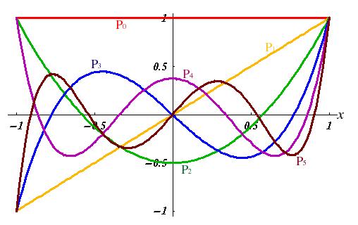
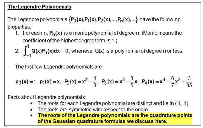
15 Note that for values of n > 2 the method of undetermined coefficients leads to nonlinear systems which are significantly more difficult. An alternate approach uses a collection of orthogonal polynomials known as the Legendre polynomials. (By orthogonal polynomials we mean that a particular integral of the product of any two different polynomials is zero.)
16
17
18
19 The simplest form of Gaussian Integration is based on the use of an optimally chosen polynomial to approximate the integrand f(x) over the interval [-1, +1]. The details of the determination of this polynomial, meaning determination of the coefficients of x in this polynomial, are beyond the scope of this presentation. The particular points at which to evaluate f(x) are the roots of the Legendre polynomials. It can be shown that the best estimate of the integral is then: where x i is a designated evaluation point, and c i is the weight of that point in the sum. If the number of points at which the function f(x) is evaluated is n, the resulting value of the integral is of the same accuracy as a simple polynomial method (such as Simpson's Rule) using about twice as many quadrature points. Thus the carefully designed choice of function evaluation points in the Gauss-Legendre form results in the same accuracy for about half the number of function evaluations, and thus at about half the computing effort.

20 Gaussian quadrature formulas are evaluated using abscissas and weights from a table like that included here. The choice of value of n is not always clear, and experimentation is useful to see the influence of choosing a different number of points. When choosing to use n points, we call the method an n-point Gaussian method.

21 Example: Consider the evaluation of the integral: whose value is 1, as we can obtain by explicit integration. Applying the 2-point Gaussian method we can calculate an approximate value for the integral. The result is , which is pretty close to the exact value of one. The calculation is simply: While this example is quite simple, the following table of values obtained for n ranging from 2 to 10 indicates how accurate the estimate of the integral is for only a few function evaluations. The table includes a column of values obtained from Simpson's rule for the same number of function evaluations. The Gauss-Legendre result is correct to almost twice the number of digits as compared to the Simpson's rule result for the same number of function evaluations.
Integration. Topic: Trapezoidal Rule. Major: General Engineering. Author: Autar Kaw, Charlie Barker.
 Integration Topic: Trapezoidal Rule Major: General Engineering Author: Autar Kaw, Charlie Barker 1 What is Integration Integration: The process of measuring the area under a function plotted on a graph.
CS 450 Numerical Analysis. Chapter 8: Numerical Integration and Differentiation
 Lecture slides based on the textbook Scientific Computing: An Introductory Survey by Michael T. Heath, copyright c 2018 by the Society for Industrial and Applied Mathematics. http://www.siam.org/books/cl80
MA2501 Numerical Methods Spring 2015
 Norwegian University of Science and Technology Department of Mathematics MA5 Numerical Methods Spring 5 Solutions to exercise set 9 Find approximate values of the following integrals using the adaptive
8.3 Numerical Quadrature, Continued
 8.3 Numerical Quadrature, Continued Ulrich Hoensch Friday, October 31, 008 Newton-Cotes Quadrature General Idea: to approximate the integral I (f ) of a function f : [a, b] R, use equally spaced nodes
Bindel, Spring 2012 Intro to Scientific Computing (CS 3220) Week 12: Monday, Apr 16. f(x) dx,
 Week 12: Monday, Apr 16. f(x) dx,") Panel integration Week 12: Monday, Apr 16 Suppose we want to compute the integral b a f(x) dx In estimating a derivative, it makes sense to use a locally accurate approximation to the function around the
Panel integration Week 12: Monday, Apr 16 Suppose we want to compute the integral b a f(x) dx In estimating a derivative, it makes sense to use a locally accurate approximation to the function around the
Numerical Integration (Quadrature) Another application for our interpolation tools!
 Another application for our interpolation tools!") Numerical Integration (Quadrature) Another application for our interpolation tools! Integration: Area under a curve Curve = data or function Integrating data Finite number of data points spacing specified
Numerical Integration (Quadrature) Another application for our interpolation tools! Integration: Area under a curve Curve = data or function Integrating data Finite number of data points spacing specified
Romberg Integration and Gaussian Quadrature
 Romberg Integration and Gaussian Quadrature P. Sam Johnson October 17, 014 P. Sam Johnson (NITK) Romberg Integration and Gaussian Quadrature October 17, 014 1 / 19 Overview We discuss two methods for integration.
Numerical integration and differentiation. Unit IV. Numerical Integration and Differentiation. Plan of attack. Numerical integration.
 Unit IV Numerical Integration and Differentiation Numerical integration and differentiation quadrature classical formulas for equally spaced nodes improper integrals Gaussian quadrature and orthogonal
COURSE Numerical integration of functions (continuation) 3.3. The Romberg s iterative generation method
 3.3. The Romberg s iterative generation method") COURSE 7 3. Numerical integration of functions (continuation) 3.3. The Romberg s iterative generation method The presence of derivatives in the remainder difficulties in applicability to practical problems
COURSE 7 3. Numerical integration of functions (continuation) 3.3. The Romberg s iterative generation method The presence of derivatives in the remainder difficulties in applicability to practical problems
Numerical Integra/on
 Numerical Integra/on Applica/ons The Trapezoidal Rule is a technique to approximate the definite integral where For 1 st order: f(a) f(b) a b Error Es/mate of Trapezoidal Rule Truncation error: From Newton-Gregory
In numerical analysis quadrature refers to the computation of definite integrals.
 Numerical Quadrature In numerical analysis quadrature refers to the computation of definite integrals. f(x) a x i x i+1 x i+2 b x A traditional way to perform numerical integration is to take a piece of
COURSE Numerical integration of functions
 COURSE 6 3. Numerical integration of functions The need: for evaluating definite integrals of functions that has no explicit antiderivatives or whose antiderivatives are not easy to obtain. Let f : [a,
PowerPoints organized by Dr. Michael R. Gustafson II, Duke University
 Part 5 Chapter 17 Numerical Integration Formulas PowerPoints organized by Dr. Michael R. Gustafson II, Duke University All images copyright The McGraw-Hill Companies, Inc. Permission required for reproduction
Numerical Integra/on
 Numerical Integra/on The Trapezoidal Rule is a technique to approximate the definite integral where For 1 st order: f(a) f(b) a b Error Es/mate of Trapezoidal Rule Truncation error: From Newton-Gregory
LECTURE 16 GAUSS QUADRATURE In general for Newton-Cotes (equispaced interpolation points/ data points/ integration points/ nodes).
.") CE 025 - Lecture 6 LECTURE 6 GAUSS QUADRATURE In general for ewton-cotes (equispaced interpolation points/ data points/ integration points/ nodes). x E x S fx dx hw' o f o + w' f + + w' f + E 84 f 0 f
CE 025 - Lecture 6 LECTURE 6 GAUSS QUADRATURE In general for ewton-cotes (equispaced interpolation points/ data points/ integration points/ nodes). x E x S fx dx hw' o f o + w' f + + w' f + E 84 f 0 f
X. Numerical Methods
 X. Numerical Methods. Taylor Approximation Suppose that f is a function defined in a neighborhood of a point c, and suppose that f has derivatives of all orders near c. In section 5 of chapter 9 we introduced
MA6452 STATISTICS AND NUMERICAL METHODS UNIT IV NUMERICAL DIFFERENTIATION AND INTEGRATION
 MA6452 STATISTICS AND NUMERICAL METHODS UNIT IV NUMERICAL DIFFERENTIATION AND INTEGRATION By Ms. K. Vijayalakshmi Assistant Professor Department of Applied Mathematics SVCE NUMERICAL DIFFERENCE: 1.NEWTON
3. Numerical integration
 3. Numerical integration... 3. One-dimensional quadratures... 3. Two- and three-dimensional quadratures... 3.3 Exact Integrals for Straight Sided Triangles... 5 3.4 Reduced and Selected Integration...
Numerical Analysis Preliminary Exam 10 am to 1 pm, August 20, 2018
 Numerical Analysis Preliminary Exam 1 am to 1 pm, August 2, 218 Instructions. You have three hours to complete this exam. Submit solutions to four (and no more) of the following six problems. Please start
Jim Lambers MAT 460/560 Fall Semester Practice Final Exam
 Jim Lambers MAT 460/560 Fall Semester 2009-10 Practice Final Exam 1. Let f(x) = sin 2x + cos 2x. (a) Write down the 2nd Taylor polynomial P 2 (x) of f(x) centered around x 0 = 0. (b) Write down the corresponding
Integration, differentiation, and root finding. Phys 420/580 Lecture 7
 Integration, differentiation, and root finding Phys 420/580 Lecture 7 Numerical integration Compute an approximation to the definite integral I = b Find area under the curve in the interval Trapezoid Rule:
Numerical Methods and Computation Prof. S.R.K. Iyengar Department of Mathematics Indian Institute of Technology Delhi
 Numerical Methods and Computation Prof. S.R.K. Iyengar Department of Mathematics Indian Institute of Technology Delhi Lecture No - 27 Interpolation and Approximation (Continued.) In our last lecture we
5 Numerical Integration & Dierentiation
 5 Numerical Integration & Dierentiation Department of Mathematics & Statistics ASU Outline of Chapter 5 1 The Trapezoidal and Simpson Rules 2 Error Formulas 3 Gaussian Numerical Integration 4 Numerical
Outline. 1 Numerical Integration. 2 Numerical Differentiation. 3 Richardson Extrapolation
 Outline Numerical Integration Numerical Differentiation Numerical Integration Numerical Differentiation 3 Michael T. Heath Scientific Computing / 6 Main Ideas Quadrature based on polynomial interpolation:
APPM/MATH Problem Set 6 Solutions
 APPM/MATH 460 Problem Set 6 Solutions This assignment is due by 4pm on Wednesday, November 6th You may either turn it in to me in class or in the box outside my office door (ECOT ) Minimal credit will
Exact and Approximate Numbers:
 Eact and Approimate Numbers: The numbers that arise in technical applications are better described as eact numbers because there is not the sort of uncertainty in their values that was described above.
18.01 EXERCISES. Unit 3. Integration. 3A. Differentials, indefinite integration. 3A-1 Compute the differentials df(x) of the following functions.
 of the following functions.") 8. EXERCISES Unit 3. Integration 3A. Differentials, indefinite integration 3A- Compute the differentials df(x) of the following functions. a) d(x 7 + sin ) b) d x c) d(x 8x + 6) d) d(e 3x sin x) e) Express
8. EXERCISES Unit 3. Integration 3A. Differentials, indefinite integration 3A- Compute the differentials df(x) of the following functions. a) d(x 7 + sin ) b) d x c) d(x 8x + 6) d) d(e 3x sin x) e) Express
Review. Numerical Methods Lecture 22. Prof. Jinbo Bi CSE, UConn
 Review Taylor Series and Error Analysis Roots of Equations Linear Algebraic Equations Optimization Numerical Differentiation and Integration Ordinary Differential Equations Partial Differential Equations
6 Lecture 6b: the Euler Maclaurin formula
 Queens College, CUNY, Department of Computer Science Numerical Methods CSCI 361 / 761 Fall 217 Instructor: Dr. Sateesh Mane c Sateesh R. Mane 217 March 26, 218 6 Lecture 6b: the Euler Maclaurin formula
(x x 0 )(x x 1 )... (x x n ) (x x 0 ) + y 0.
(x x 1 )... (x x n ) (x x 0 ) + y 0.") > 5. Numerical Integration Review of Interpolation Find p n (x) with p n (x j ) = y j, j = 0, 1,,..., n. Solution: p n (x) = y 0 l 0 (x) + y 1 l 1 (x) +... + y n l n (x), l k (x) = n j=1,j k Theorem Let
> 5. Numerical Integration Review of Interpolation Find p n (x) with p n (x j ) = y j, j = 0, 1,,..., n. Solution: p n (x) = y 0 l 0 (x) + y 1 l 1 (x) +... + y n l n (x), l k (x) = n j=1,j k Theorem Let
5.3 Definite Integrals and Antiderivatives
 5.3 Definite Integrals and Antiderivatives Objective SWBAT use properties of definite integrals, average value of a function, mean value theorem for definite integrals, and connect differential and integral
April 15 Math 2335 sec 001 Spring 2014
 April 15 Math 2335 sec 001 Spring 2014 Trapezoid and Simpson s Rules I(f ) = b a f (x) dx Trapezoid Rule: If [a, b] is divided into n equally spaced subintervals of length h = (b a)/n, then I(f ) T n (f
12.0 Properties of orthogonal polynomials
 12.0 Properties of orthogonal polynomials In this section we study orthogonal polynomials to use them for the construction of quadrature formulas investigate projections on polynomial spaces and their
NUMERICAL INTEGRATION. By : Dewi Rachmatin
 NUMERICAL INTEGRATION By : Dewi Rachmatin The Trapezoidal Rule Theorem (Trapezoidal Rule) Consider y=f(x) over [x 0,x 1 ], where x 1 =x 0 +h. The trapezoidal rule is This is an numerical approximation
A New Integration Method Providing the Accuracy of Gauss-Legendre with Error Estimation Capability (rev.)
") July 7, 2003 A New Integration Method Providing the Accuracy of Gauss-Legendre with Error Estimation Capability (rev.) by C. Bond, c 2002 1 Background One of the best methods for non-adaptive numerical
July 7, 2003 A New Integration Method Providing the Accuracy of Gauss-Legendre with Error Estimation Capability (rev.) by C. Bond, c 2002 1 Background One of the best methods for non-adaptive numerical
Differentiation and Integration
 Differentiation and Integration (Lectures on Numerical Analysis for Economists II) Jesús Fernández-Villaverde 1 and Pablo Guerrón 2 February 12, 2018 1 University of Pennsylvania 2 Boston College Motivation
Numerical Integration exact integration is not needed to achieve the optimal convergence rate of nite element solutions ([, 9, 11], and Chapter 7). In
![Numerical Integration exact integration is not needed to achieve the optimal convergence rate of nite element solutions ([, 9, 11], and Chapter 7). In](/thumbs/80/80480766.jpg "Numerical Integration exact integration is not needed to achieve the optimal convergence rate of nite element solutions ([, 9, 11], and Chapter 7). In") Chapter 6 Numerical Integration 6.1 Introduction After transformation to a canonical element,typical integrals in the element stiness or mass matrices (cf. (5.5.8)) have the forms Q = T ( )N s Nt det(j
Chapter 6 Numerical Integration 6.1 Introduction After transformation to a canonical element,typical integrals in the element stiness or mass matrices (cf. (5.5.8)) have the forms Q = T ( )N s Nt det(j
Ch. 03 Numerical Quadrature. Andrea Mignone Physics Department, University of Torino AA
 Ch. 03 Numerical Quadrature Andrea Mignone Physics Department, University of Torino AA 2017-2018 Numerical Quadrature In numerical analysis quadrature refers to the computation of definite integrals. y
Scientific Computing
 2301678 Scientific Computing Chapter 2 Interpolation and Approximation Paisan Nakmahachalasint Paisan.N@chula.ac.th Chapter 2 Interpolation and Approximation p. 1/66 Contents 1. Polynomial interpolation
Numerical techniques to solve equations
 Programming for Applications in Geomatics, Physical Geography and Ecosystem Science (NGEN13) Numerical techniques to solve equations vaughan.phillips@nateko.lu.se Vaughan Phillips Associate Professor,
8.5 Taylor Polynomials and Taylor Series
 8.5. TAYLOR POLYNOMIALS AND TAYLOR SERIES 50 8.5 Taylor Polynomials and Taylor Series Motivating Questions In this section, we strive to understand the ideas generated by the following important questions:
Physics 200 Lecture 4. Integration. Lecture 4. Physics 200 Laboratory
 Physics 2 Lecture 4 Integration Lecture 4 Physics 2 Laboratory Monday, February 21st, 211 Integration is the flip-side of differentiation in fact, it is often possible to write a differential equation
Mathematics for Engineers. Numerical mathematics
 Mathematics for Engineers Numerical mathematics Integers Determine the largest representable integer with the intmax command. intmax ans = int32 2147483647 2147483647+1 ans = 2.1475e+09 Remark The set
Digital Wideband Integrators with Matching Phase and Arbitrarily Accurate Magnitude Response (Extended Version)
") Digital Wideband Integrators with Matching Phase and Arbitrarily Accurate Magnitude Response (Extended Version) Ça gatay Candan Department of Electrical Engineering, METU, Ankara, Turkey ccandan@metu.edu.tr
Digital Wideband Integrators with Matching Phase and Arbitrarily Accurate Magnitude Response (Extended Version) Ça gatay Candan Department of Electrical Engineering, METU, Ankara, Turkey ccandan@metu.edu.tr
Numerical Methods I: Numerical Integration/Quadrature
 1/20 Numerical Methods I: Numerical Integration/Quadrature Georg Stadler Courant Institute, NYU stadler@cims.nyu.edu November 30, 2017 umerical integration 2/20 We want to approximate the definite integral
Gregory's quadrature method
 Gregory's quadrature method Gregory's method is among the very first quadrature formulas ever described in the literature, dating back to James Gregory (638-675). It seems to have been highly regarded
4.9 APPROXIMATING DEFINITE INTEGRALS
 4.9 Approximating Definite Integrals Contemporary Calculus 4.9 APPROXIMATING DEFINITE INTEGRALS The Fundamental Theorem of Calculus tells how to calculate the exact value of a definite integral IF the
Principles of Scientific Computing Local Analysis
 Principles of Scientific Computing Local Analysis David Bindel and Jonathan Goodman last revised January 2009, printed February 25, 2009 1 Among the most common computational tasks are differentiation,
NUMERICAL METHODS. x n+1 = 2x n x 2 n. In particular: which of them gives faster convergence, and why? [Work to four decimal places.
 NUMERICAL METHODS 1. Rearranging the equation x 3 =.5 gives the iterative formula x n+1 = g(x n ), where g(x) = (2x 2 ) 1. (a) Starting with x = 1, compute the x n up to n = 6, and describe what is happening.
BACHELOR OF COMPUTER APPLICATIONS (BCA) (Revised) Term-End Examination December, 2015 BCS-054 : COMPUTER ORIENTED NUMERICAL TECHNIQUES
 (Revised) Term-End Examination December, 2015 BCS-054 : COMPUTER ORIENTED NUMERICAL TECHNIQUES") No. of Printed Pages : 5 BCS-054 BACHELOR OF COMPUTER APPLICATIONS (BCA) (Revised) Term-End Examination December, 2015 058b9 BCS-054 : COMPUTER ORIENTED NUMERICAL TECHNIQUES Time : 3 hours Maximum Marks
No. of Printed Pages : 5 BCS-054 BACHELOR OF COMPUTER APPLICATIONS (BCA) (Revised) Term-End Examination December, 2015 058b9 BCS-054 : COMPUTER ORIENTED NUMERICAL TECHNIQUES Time : 3 hours Maximum Marks
MTH101 Calculus And Analytical Geometry Lecture Wise Questions and Answers For Final Term Exam Preparation
 MTH101 Calculus And Analytical Geometry Lecture Wise Questions and Answers For Final Term Exam Preparation Lecture No 23 to 45 Complete and Important Question and answer 1. What is the difference between
Math 107H Fall 2008 Course Log and Cumulative Homework List
 Date: 8/25 Sections: 5.4 Math 107H Fall 2008 Course Log and Cumulative Homework List Log: Course policies. Review of Intermediate Value Theorem. The Mean Value Theorem for the Definite Integral and the
Page 404. Lecture 22: Simple Harmonic Oscillator: Energy Basis Date Given: 2008/11/19 Date Revised: 2008/11/19
 Page 404 Lecture : Simple Harmonic Oscillator: Energy Basis Date Given: 008/11/19 Date Revised: 008/11/19 Coordinate Basis Section 6. The One-Dimensional Simple Harmonic Oscillator: Coordinate Basis Page
Engg. Math. II (Unit-IV) Numerical Analysis
 Numerical Analysis") Dr. Satish Shukla of 33 Engg. Math. II (Unit-IV) Numerical Analysis Syllabus. Interpolation and Curve Fitting: Introduction to Interpolation; Calculus of Finite Differences; Finite Difference and Divided
Dr. Satish Shukla of 33 Engg. Math. II (Unit-IV) Numerical Analysis Syllabus. Interpolation and Curve Fitting: Introduction to Interpolation; Calculus of Finite Differences; Finite Difference and Divided
Infinite Series. 1 Introduction. 2 General discussion on convergence
 Infinite Series 1 Introduction I will only cover a few topics in this lecture, choosing to discuss those which I have used over the years. The text covers substantially more material and is available for
Numerical Methods. King Saud University
 Numerical Methods King Saud University Aims In this lecture, we will... find the approximate solutions of derivative (first- and second-order) and antiderivative (definite integral only). Numerical Differentiation
To find an approximate value of the integral, the idea is to replace, on each subinterval
 Module 6 : Definition of Integral Lecture 18 : Approximating Integral : Trapezoidal Rule [Section 181] Objectives In this section you will learn the following : Mid point and the Trapezoidal methods for
GAUSS-LAGUERRE AND GAUSS-HERMITE QUADRATURE ON 64, 96 AND 128 NODES
 GAUSS-LAGUERRE AND GAUSS-HERMITE QUADRATURE ON 64, 96 AND 128 NODES RICHARD J. MATHAR Abstract. The manuscript provides tables of abscissae and weights for Gauss- Laguerre integration on 64, 96 and 128
Fixed point iteration and root finding
 Fixed point iteration and root finding The sign function is defined as x > 0 sign(x) = 0 x = 0 x < 0. It can be evaluated via an iteration which is useful for some problems. One such iteration is given
NUMERICAL COMPUTATION IN SCIENCE AND ENGINEERING
 NUMERICAL COMPUTATION IN SCIENCE AND ENGINEERING C. Pozrikidis University of California, San Diego New York Oxford OXFORD UNIVERSITY PRESS 1998 CONTENTS Preface ix Pseudocode Language Commands xi 1 Numerical
Answers to Homework 9: Numerical Integration
 Math 8A Spring Handout # Sergey Fomel April 3, Answers to Homework 9: Numerical Integration. a) Suppose that the function f x) = + x ) is known at three points: x =, x =, and x 3 =. Interpolate the function
Scientific Computing: An Introductory Survey
 Scientific Computing: An Introductory Survey Chapter 7 Interpolation Prof. Michael T. Heath Department of Computer Science University of Illinois at Urbana-Champaign Copyright c 2002. Reproduction permitted
Outline. 1 Interpolation. 2 Polynomial Interpolation. 3 Piecewise Polynomial Interpolation
 Outline Interpolation 1 Interpolation 2 3 Michael T. Heath Scientific Computing 2 / 56 Interpolation Motivation Choosing Interpolant Existence and Uniqueness Basic interpolation problem: for given data
Multistage Methods I: Runge-Kutta Methods
 Multistage Methods I: Runge-Kutta Methods Varun Shankar January, 0 Introduction Previously, we saw that explicit multistep methods (AB methods) have shrinking stability regions as their orders are increased.
Pascal s Triangle on a Budget. Accuracy, Precision and Efficiency in Sparse Grids
 Covering : Accuracy, Precision and Efficiency in Sparse Grids https://people.sc.fsu.edu/ jburkardt/presentations/auburn 2009.pdf... John Interdisciplinary Center for Applied Mathematics & Information Technology
Method of Finite Elements I
 Method of Finite Elements I PhD Candidate - Charilaos Mylonas HIL H33.1 and Boundary Conditions, 26 March, 2018 Institute of Structural Engineering Method of Finite Elements I 1 Outline 1 2 Penalty method
Chapter 5 - Quadrature
 Chapter 5 - Quadrature The Goal: Adaptive Quadrature Historically in mathematics, quadrature refers to the act of trying to find a square with the same area of a given circle. In mathematical computing,
Practice Exam 2 (Solutions)
") Math 5, Fall 7 Practice Exam (Solutions). Using the points f(x), f(x h) and f(x + h) we want to derive an approximation f (x) a f(x) + a f(x h) + a f(x + h). (a) Write the linear system that you must solve
Math 5, Fall 7 Practice Exam (Solutions). Using the points f(x), f(x h) and f(x + h) we want to derive an approximation f (x) a f(x) + a f(x h) + a f(x + h). (a) Write the linear system that you must solve
MATHEMATICAL FORMULAS AND INTEGRALS
 MATHEMATICAL FORMULAS AND INTEGRALS ALAN JEFFREY Department of Engineering Mathematics University of Newcastle upon Tyne Newcastle upon Tyne United Kingdom Academic Press San Diego New York Boston London
PHYS-4007/5007: Computational Physics Course Lecture Notes Appendix G
 PHYS-4007/5007: Computational Physics Course Lecture Notes Appendix G Dr. Donald G. Luttermoser East Tennessee State University Version 7.0 Abstract These class notes are designed for use of the instructor
In manycomputationaleconomicapplications, one must compute thede nite n
 Chapter 6 Numerical Integration In manycomputationaleconomicapplications, one must compute thede nite n integral of a real-valued function f de ned on some interval I of
Lecture Note 3: Interpolation and Polynomial Approximation. Xiaoqun Zhang Shanghai Jiao Tong University
 Lecture Note 3: Interpolation and Polynomial Approximation Xiaoqun Zhang Shanghai Jiao Tong University Last updated: October 10, 2015 2 Contents 1.1 Introduction................................ 3 1.1.1
(f(x) P 3 (x)) dx. (a) The Lagrange formula for the error is given by
 P 3 (x)) dx. (a) The Lagrange formula for the error is given by") 1. QUESTION (a) Given a nth degree Taylor polynomial P n (x) of a function f(x), expanded about x = x 0, write down the Lagrange formula for the truncation error, carefully defining all its elements. How
1. QUESTION (a) Given a nth degree Taylor polynomial P n (x) of a function f(x), expanded about x = x 0, write down the Lagrange formula for the truncation error, carefully defining all its elements. How
Lecture 28 The Main Sources of Error
 Lecture 28 The Main Sources of Error Truncation Error Truncation error is defined as the error caused directly by an approximation method For instance, all numerical integration methods are approximations
Math 1132 Practice Exam 1 Spring 2016
 University of Connecticut Department of Mathematics Math 32 Practice Exam Spring 206 Name: Instructor Name: TA Name: Section: Discussion Section: Read This First! Please read each question carefully. Show
x x2 2 + x3 3 x4 3. Use the divided-difference method to find a polynomial of least degree that fits the values shown: (b)
") Numerical Methods - PROBLEMS. The Taylor series, about the origin, for log( + x) is x x2 2 + x3 3 x4 4 + Find an upper bound on the magnitude of the truncation error on the interval x.5 when log( + x)
Numerical Methods - PROBLEMS. The Taylor series, about the origin, for log( + x) is x x2 2 + x3 3 x4 4 + Find an upper bound on the magnitude of the truncation error on the interval x.5 when log( + x)
arxiv: v1 [physics.comp-ph] 22 Jul 2010
![arxiv: v1 [physics.comp-ph] 22 Jul 2010](/thumbs/71/65800290.jpg "arxiv: v1 [physics.comp-ph] 22 Jul 2010") Gaussian integration with rescaling of abscissas and weights arxiv:007.38v [physics.comp-ph] 22 Jul 200 A. Odrzywolek M. Smoluchowski Institute of Physics, Jagiellonian University, Cracov, Poland Abstract
Gaussian integration with rescaling of abscissas and weights arxiv:007.38v [physics.comp-ph] 22 Jul 200 A. Odrzywolek M. Smoluchowski Institute of Physics, Jagiellonian University, Cracov, Poland Abstract
MATH 1242 FINAL EXAM Spring,
 MATH 242 FINAL EXAM Spring, 200 Part I (MULTIPLE CHOICE, NO CALCULATORS).. Find 2 4x3 dx. (a) 28 (b) 5 (c) 0 (d) 36 (e) 7 2. Find 2 cos t dt. (a) 2 sin t + C (b) 2 sin t + C (c) 2 cos t + C (d) 2 cos t
Contents. I Basic Methods 13
 Preface xiii 1 Introduction 1 I Basic Methods 13 2 Convergent and Divergent Series 15 2.1 Introduction... 15 2.1.1 Power series: First steps... 15 2.1.2 Further practical aspects... 17 2.2 Differential
Quantum Mechanics-I Prof. Dr. S. Lakshmi Bala Department of Physics Indian Institute of Technology, Madras. Lecture - 21 Square-Integrable Functions
 Quantum Mechanics-I Prof. Dr. S. Lakshmi Bala Department of Physics Indian Institute of Technology, Madras Lecture - 21 Square-Integrable Functions (Refer Slide Time: 00:06) (Refer Slide Time: 00:14) We
ONE - DIMENSIONAL INTEGRATION
 Chapter 4 ONE - DIMENSIONA INTEGRATION 4. Introduction Since the finite element method is based on integral relations it is logical to expect that one should strive to carry out the integrations as efficiently
MA 3021: Numerical Analysis I Numerical Differentiation and Integration
 MA 3021: Numerical Analysis I Numerical Differentiation and Integration Suh-Yuh Yang ( 楊肅煜 ) Department of Mathematics, National Central University Jhongli District, Taoyuan City 32001, Taiwan syyang@math.ncu.edu.tw
DIFFERENTIATION RULES
 3 DIFFERENTIATION RULES DIFFERENTIATION RULES We have: Seen how to interpret derivatives as slopes and rates of change Seen how to estimate derivatives of functions given by tables of values Learned how
Physics 115/242 Romberg Integration
 Physics 5/242 Romberg Integration Peter Young In this handout we will see how, starting from the trapezium rule, we can obtain much more accurate values for the integral by repeatedly eliminating the leading
Chapter 8: Techniques of Integration
 Chapter 8: Techniques of Integration Section 8.1 Integral Tables and Review a. Important Integrals b. Example c. Integral Tables Section 8.2 Integration by Parts a. Formulas for Integration by Parts b.
Virtual University of Pakistan
 Virtual University of Pakistan File Version v.0.0 Prepared For: Final Term Note: Use Table Of Content to view the Topics, In PDF(Portable Document Format) format, you can check Bookmarks menu Disclaimer:
Research Computing with Python, Lecture 7, Numerical Integration and Solving Ordinary Differential Equations
 Research Computing with Python, Lecture 7, Numerical Integration and Solving Ordinary Differential Equations Ramses van Zon SciNet HPC Consortium November 25, 2014 Ramses van Zon (SciNet HPC Consortium)Research
t dt Estimate the value of the integral with the trapezoidal rule. Use n = 4.
 Trapezoidal Rule We have already found the value of an integral using rectangles in the first lesson of this module. In this section we will again be estimating the value of an integral using geometric
Department of Applied Mathematics and Theoretical Physics. AMA 204 Numerical analysis. Exam Winter 2004
 Department of Applied Mathematics and Theoretical Physics AMA 204 Numerical analysis Exam Winter 2004 The best six answers will be credited All questions carry equal marks Answer all parts of each question
Spring 2012 Introduction to numerical analysis Class notes. Laurent Demanet
 18.330 Spring 2012 Introduction to numerical analysis Class notes Laurent Demanet Draft April 25, 2014 2 Preface Good additional references are Burden and Faires, Introduction to numerical analysis Suli
Some notes on Chapter 8: Polynomial and Piecewise-polynomial Interpolation
 Some notes on Chapter 8: Polynomial and Piecewise-polynomial Interpolation See your notes. 1. Lagrange Interpolation (8.2) 1 2. Newton Interpolation (8.3) different form of the same polynomial as Lagrange
d 1 µ 2 Θ = 0. (4.1) consider first the case of m = 0 where there is no azimuthal dependence on the angle φ.
 consider first the case of m = 0 where there is no azimuthal dependence on the angle φ.") 4 Legendre Functions In order to investigate the solutions of Legendre s differential equation d ( µ ) dθ ] ] + l(l + ) m dµ dµ µ Θ = 0. (4.) consider first the case of m = 0 where there is no azimuthal
4 Legendre Functions In order to investigate the solutions of Legendre s differential equation d ( µ ) dθ ] ] + l(l + ) m dµ dµ µ Θ = 0. (4.) consider first the case of m = 0 where there is no azimuthal
NATIONAL UNIVERSITY OF SINGAPORE PC5215 NUMERICAL RECIPES WITH APPLICATIONS. (Semester I: AY ) Time Allowed: 2 Hours
 Time Allowed: 2 Hours") NATIONAL UNIVERSITY OF SINGAPORE PC5215 NUMERICAL RECIPES WITH APPLICATIONS (Semester I: AY 2014-15) Time Allowed: 2 Hours INSTRUCTIONS TO CANDIDATES 1. Please write your student number only. 2. This examination
NATIONAL UNIVERSITY OF SINGAPORE PC5215 NUMERICAL RECIPES WITH APPLICATIONS (Semester I: AY 2014-15) Time Allowed: 2 Hours INSTRUCTIONS TO CANDIDATES 1. Please write your student number only. 2. This examination
Numerical Analysis Exam with Solutions
 Numerical Analysis Exam with Solutions Richard T. Bumby Fall 000 June 13, 001 You are expected to have books, notes and calculators available, but computers of telephones are not to be used during the
Extrapolation in Numerical Integration. Romberg Integration
 Extrapolation in Numerical Integration Romberg Integration Matthew Battaglia Joshua Berge Sara Case Yoobin Ji Jimu Ryoo Noah Wichrowski Introduction Extrapolation: the process of estimating beyond the
TABLE OF CONTENTS INTRODUCTION, APPROXIMATION & ERRORS 1. Chapter Introduction to numerical methods 1 Multiple-choice test 7 Problem set 9
 TABLE OF CONTENTS INTRODUCTION, APPROXIMATION & ERRORS 1 Chapter 01.01 Introduction to numerical methods 1 Multiple-choice test 7 Problem set 9 Chapter 01.02 Measuring errors 11 True error 11 Relative
n = 4: 0 2( ) (4 0) ( t 2.67%) 8
 (4 0) ( t 2.67%) 8") 1 CHAPTER 19 19.1 A table of integrals can be consulted to determine 1 tanh dx ln cosh ax a Therefore, t gm gc gm gc d gm m gc d tanh t dt ln cosh t c d m cd gcd m d ln cosh gc d t ln cosh() m Since cosh()
1 CHAPTER 19 19.1 A table of integrals can be consulted to determine 1 tanh dx ln cosh ax a Therefore, t gm gc gm gc d gm m gc d tanh t dt ln cosh t c d m cd gcd m d ln cosh gc d t ln cosh() m Since cosh()
Algebra I. abscissa the distance along the horizontal axis in a coordinate graph; graphs the domain.
 Algebra I abscissa the distance along the horizontal axis in a coordinate graph; graphs the domain. absolute value the numerical [value] when direction or sign is not considered. (two words) additive inverse
Numerical Integration of Functions
 Numerical Integration of Functions Berlin Chen Department of Computer Science & Information Engineering National Taiwan Normal University Reference: 1. Applied Numerical Methods with MATLAB for Engineers,
19.4 Spline Interpolation
 c9-b.qxd 9/6/5 6:4 PM Page 8 8 CHAP. 9 Numerics in General 9.4 Spline Interpolation Given data (function values, points in the xy-plane) (x, ƒ ), (x, ƒ ),, (x n, ƒ n ) can be interpolated by a polynomial