Vector Field Topology. Ronald Peikert SciVis Vector Field Topology 8-1
|
|
|
- Leon Cannon
- 6 years ago
- Views:
Transcription
1 Vector Field Topology Ronald Peikert SciVis Vector Field Topology 8-1
2 Vector fields as ODEs What are conditions for existence and uniqueness of streamlines? For the initial value problem i x ( t) = v x( t) ( ) x ( ) t = x 0 0 ( ) v x a solution exists if the velocity field is continuous. The solution is unique if the field is Lipschitz-continuous, i.e. if there is a constant M such that ( ) ( ) M vx vx x x for all x in a neighborhood of x. Ronald Peikert SciVis Vector Field Topology 8-2
3 Vector fields as ODEs Lipschitz-continuous is stronger than continuous (C 0 ) but weaker than continuously differentiable (C 1 ). Important for scientific visualization: piecewise multilinear functions are Lipschitz-continuous in particular cellwise bi- or trilinear interpolation is Lipschitzcontinuous Consequence: Numerical vector fields do have unique streamlines, but analytic vector fields don't necessarily. Ronald Peikert SciVis Vector Field Topology 8-3
4 Vector fields as ODEs Example: for the vector field ( ) ( ) ( ) v x ( ) ( 2/3 u x, y, v x, y 1,3y ) = = the initial value problem i x ( t) = v x( t) ( ) has the two solutions x ( t ) = ( x + t, 0 ) x red blue 0 x () ( 3 t = x ) 0 + t, t ( 0 ) = x0 Both are streamlines seeded at the point. p ( x,0 0 ) 0,0 Ronald Peikert SciVis Vector Field Topology 8-4
5 Special streamlines x( t) It is possible that a streamline maps two different times t and t' to the same point: x t = x t' = x ( ) ( ) 1 There are two types of such special streamlines: stationary yp points: If vx ( 1 ) = 0, then the streamline degenerates to a single point x t = x t R ( ) ( ) ( ) periodic orbits: If vx, then the streamline is periodic: 1 0 All other streamlines are called regular streamlines. 1 ( t+ kt) = ( t) ( t, k ) x x R Z Ronald Peikert SciVis Vector Field Topology 8-5
6 Special streamlines Regular streamlines can converge to stationary points or periodic orbits, in either positive or negative time. However, because of the uniqueness, a regular streamline cannot contain a stationary point or periodic orbit. Examples: convergence to a stationary point a periodic orbit Ronald Peikert SciVis Vector Field Topology 8-6
7 Critical points A stationary point x c is called a critical point if the velocity gradient J= v x at x c is regular (is a non-singular matrix, has nonzero ( ) determinant). Near a critical point, the field can be approximated by its linearizationi Properties of critical points: ( ) ( 2 ) c + = + O v x x Jx x in a neighborhood, the field takes all possible directions critical points are isolated (as opposed to general stationary points, e.g. points on a no slip boundary) Ronald Peikert SciVis Vector Field Topology 8-7
8 Critical points Critical points can have different types, depending on the eigenvalues of J, more precisely on the signs of the real parts of the eigenvalues. We define an important subclass: A critical point is called hyperbolic if all eigenvalues of J have nonzero real parts. The main property of hyperbolic critical points is structural stability: Adding a small perturbation to v(x) does not change the topology of the nearby streamlines. Ronald Peikert SciVis Vector Field Topology 8-8
9 Critical points in 2D Hyperbolic critical points in 2D can be classified as follows: two real eigenvalues: both positive: node source both negative: node sink different signs: saddle two conjugate complex eigenvalues: positive real parts: focus source negative real parts: focus sink Ronald Peikert SciVis Vector Field Topology 8-9
10 Critical points in 2D In 2D the eigenvalues are the zeros of 2 x px q + + = 0 where p and q are the two invariants: i ( λ λ ) p = trace( J) = + q = det( J ) = λλ 1 2 The eigenvalues are complex exactly if the discriminant is negative D = p 4 q It follows: critical point types depend on signs of p,q and D hyperbolic points have either q < 0, or q > 0and p 0 Ronald Peikert SciVis Vector Field Topology 8-10
11 Critical points in 2D The p-q chart (hyperbolic types printed in red) q=p 2 /4 q D<0 (complex eigenvalues) D=0 D>0 (real eigenvalues) focus source focus sink node focus source node source center node focus sink node sink line source shear line sink p saddle Ronald Peikert SciVis Vector Field Topology 8-11
12 Node source positive trace positive determinant positive discriminant Example J = = A A Ronald Peikert SciVis Vector Field Topology 8-12
13 Node sink negative trace positive determinant positive discriminant Example J = = A A Ronald Peikert SciVis Vector Field Topology 8-13
14 Saddle any trace negative determinant positive discriminant Example J = = A A Ronald Peikert SciVis Vector Field Topology 8-14
15 Focus source positive trace counter-clockwise if positive determinant v x u y >0 negative discriminant Example J = = A A Ronald Peikert SciVis Vector Field Topology 8-15
16 Focus sink negative trace counter-clockwise if positive determinant v x u y >0 negative discriminant Example J = = A A Ronald Peikert SciVis Vector Field Topology 8-16
17 Node focus source positive trace between node source positive determinant and focus source zero discriminant (double real eigenvalue) Example J = = A A Ronald Peikert SciVis Vector Field Topology 8-17
18 Star source Special case of node focus source: diagonal matrix Example J = = =λ Ronald Peikert SciVis Vector Field Topology 8-18
19 Nonhyperbolic critical points If the eigenvalues have zero real parts but are nonzero (eigenvalues are purely imaginary), the critical point is the boundary case between focus source and focus sink. This type of critical point is called a center. Depending on the higher derivatives, it can behave as a source or as a sink. Because a center is nonhyperbolic, it is not structurally t stable in general perturbation but structurally t stable if the field is divergence-free. Ronald Peikert SciVis Vector Field Topology 8-19
20 Center zero trace counter-clockwise if positive determinant v x u y >0 negative discriminant Example J = = A A Ronald Peikert SciVis Vector Field Topology 8-20
21 Other stationary points Other stationary points in 2D: If J is a singular matrix, the following stationary ti (but not critical!) points are possible: if a single eigenvalue is zero: line source, line sink if both eigenvalues are zero : pure shear Ronald Peikert SciVis Vector Field Topology 8-21
22 Line source positive trace zero determinant Example J = = A A Ronald Peikert SciVis Vector Field Topology 8-22
23 Pure shear zero trace zero determinant Example J = = A A Ronald Peikert SciVis Vector Field Topology 8-23
24 The topological skeleton The topological skeleton consists of all periodic orbits and all streamlines converging (in either direction of time) to a saddle point (separatrix of the saddle), or a critical point on a no-slip boundary It provides a kind of segmentation of the 2D vector field Examples: Ronald Peikert SciVis Vector Field Topology 8-24
25 The topological skeleton Example: irrotational vector fields. An irrotational (conservative) vector field is the gradient of a scalar field (its potential). Skeleton of an irrotational vector field: watershed image of its potential field. Discussion: watersheds are topologically defined, integration required height ridges are geometrically defined, locally detectable Ronald Peikert SciVis Vector Field Topology 8-25


26 The topological skeleton Example: LIC and topology-based visualization (skeleton plus a few extra streamlines). Ronald Peikert SciVis Vector Field Topology 8-26


27 The topological skeleton Example: topological skeleton of a surface flow image credit: A. Globus Ronald Peikert SciVis Vector Field Topology 8-27
28 Critical points in 3D Hyperbolic critical points in 3D can be classified as follows: three real eigenvalues: all positive: source two positive, one negative: 1:2 saddle (1 in, 2 out) one positive, two negative: 2:1 saddle (2 in, 1 out) all negative: sink one real, two complex eigenvalues: positive real eigenvalue, positive real parts: spiral source positive real eigenvalue, negative real parts : 2:1 spiral saddle negative real eigenvalue, positive real parts : 1:2 spiral saddle negative real eigenvalue, negative real parts : spiral sink Ronald Peikert SciVis Vector Field Topology 8-28
29 Critical points in 3D Types of hyperbolic critical points in 3D source spiral source 2:1 saddle 2:1 spiral saddle The other 4 types are obtained by reversing arrows Ronald Peikert SciVis Vector Field Topology 8-29
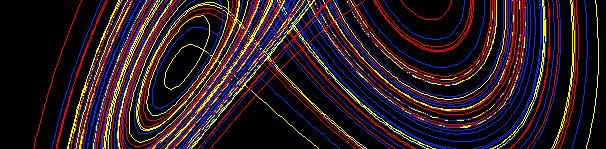
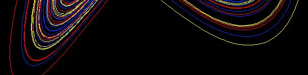
30 Example: The Lorenz attractor The Lorenz attractor v ( ) has 3 critical points: ( 10 y x, 28 x y xz, xy 8z 3) = a 2:1 saddle P 0 at ( 0,0,0, ) with eigenvalues { 22.83, 2.67, 11.82} p 1 2 two 1:2 spiral saddles P 1 and P 2 ( ) ( 6 2, 6 2, 27) at 6 2, 6 2, 27 and with eigenvalues { 13.85, 0.09 ± 10.19i } with eigenvalues Ronald Peikert SciVis Vector Field Topology 8-30
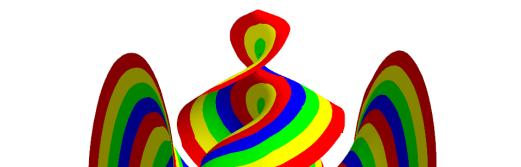
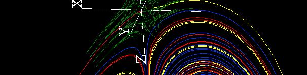


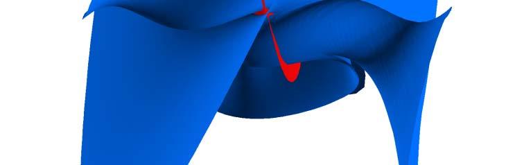

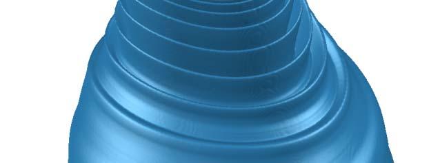
31 Streamlines Example: The Lorenz attractor Streamsurfaces (2D separatrices) stable manifold W s (P 0 ) W u (P 1 ) W s (P 0 ) W u (P 2 ) Ronald Peikert SciVis Vector Field Topology 8-31
32 Visualization based on 3D critical points Example: Flow over delta wing, glyphs (icons) for critical point types, 1D separatrices ("topological vortex cores"). Discussion: Vortex core may not contain critical points. image: A.Globus Ronald Peikert SciVis Vector Field Topology 8-32
33 Periodic orbits Poincaré map of a periodic orbit in 3D: Choose a point x 0 on the periodic orbit Choose an open circular disk D centered at x 0 on a plane which is not tangential to the flow, and small enough that the periodic orbit intersects D only in x 0 Any streamline seeded at a point x D which intersects D a next time at a point x D defines a mapping from x to x' There exists a smaller open disk D0 D centered at x 0 such that this mapping is defined for all points x D 0. This is the Poincaré map. Ronald Peikert SciVis Vector Field Topology 8-33
34 Periodic orbits Using coordinates on the plane of D and with origin at x 0, the Poincaré map can now be linearized: where P is 2x2 matrix. x Px Important fact about Poincaré maps: The eigenvalues of P are independent of the choice of x 0 on the periodic orbit the orientation of the plane of D the choice of coordinates for the plane A periodic orbit is called hyperbolic, if its eigenvalues lie off the complex unit circle. Hyperbolic p.o. are structurally stable. Ronald Peikert SciVis Vector Field Topology 8-34
35 Periodic orbits Hyperbolic periodic orbits in 3D can be classified as follows: Two real eigenvalues: both outside the unit circle: source p.o. both inside the unit circle: sink p.o. one outside, one inside: both positive: both negative: saddle p.o. twisted saddle p.o. Two complex conjugate eigenvalues: both outside the unit circle: spiral source p.o. both inside the unit circle: spiral sink p.o. Ronald Peikert SciVis Vector Field Topology 8-35
36 Periodic orbits Types of hyperbolic periodic orbits in 3D source p.o. spiral source p.o. saddle p.o. twisted saddle p.o. Types sink and spiral sink are obtained by reversing arrows. Ronald Peikert SciVis Vector Field Topology 8-36


.")
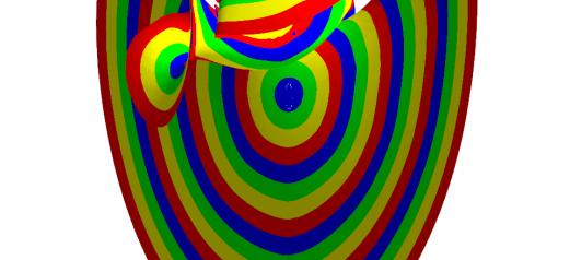
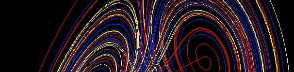
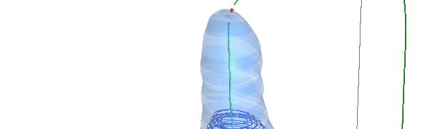
37 Periodic orbits Example: Flow in Pelton distributor ring. Critical point of spiral saddle type and p.o. of twisted saddle type. Stable (yellow, red) and unstable (black, blue) manifolds. Streamlines and streamsurfaces (manually seeded). Ronald Peikert SciVis Vector Field Topology 8-37
38 Saddle connectors The topological skeleton of 3D vector fields contains 1D and 2D separatrices of (spiral) saddles. Not directly usable for visualization (too much occlusion). Alternative: only show intersection curves of 2D separatrices. Two types of saddle connectors: heteroclinic orbit: connects two (spiral) saddles homoclinic orbits: connects a (spiral) saddle with itself Idea: a 1D "skeleton" is obtained, not providing a segmentation, but indicating flow between pairs of saddles Ronald Peikert SciVis Vector Field Topology 8-38


39 Saddle connectors Comparison: icons / full topological skeleton / saddle connectors Flow past a cylinder: Image credit: H. Theisel Ronald Peikert SciVis Vector Field Topology 8-39
40 Saddle connectors In rotational flow, a connected pair of spiral saddles can describe a vortex breakdown bubble. P 1 (2:1 spiral saddle) ideal case: W s (P 1 ) coincides with W u (P 2 ) no saddle connector P 2 (1:2 spiral saddle) perturbed case: transversal intersection of W s (P 1 ) and W u (P 2 ) saddle connector consists of two streamlines P 2 P 1 Image credit: Krasny/Nitsche Ronald Peikert SciVis Vector Field Topology 8-40
.")
41 Saddle connectors 3D view If v is velocity field of a fluid: Folds must have constant mass flux. Image credit: Sotiropoulos et al. ρv dn ρωar Close to P 1 or P 2 this is approximately (density * angular velocity * cross section area * radius). It follows: cross section area ~ 1/radius Consequence: Shilnikov chaos Ronald Peikert SciVis Vector Field Topology 8-41
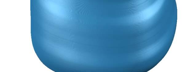
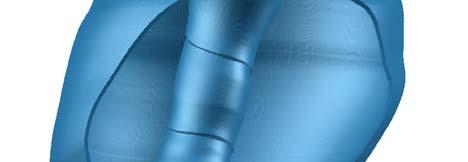
42 Saddle connectors Experimental photograph h of a vortex breakdown bubble Vortex breakdown bubble in flow over delta wing, visualization by streamsurfaces (not topology-based) Image credit: Sotiropoulos et al. Image credit: C. Garth Ronald Peikert SciVis Vector Field Topology 8-42

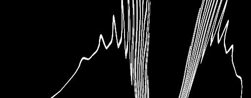

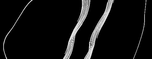
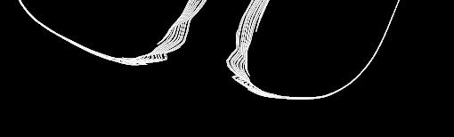
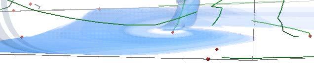
43 Saddle connectors Vortex breakdown bubble found in CFD data of Francis draft tube: Ronald Peikert SciVis Vector Field Topology 8-43
8 Vector Field Topology
 Vector fields as ODEs What are conditions for eistence and uniqueness of streamlines? 8 Vector Field Topology For the initial value problem ( t) = v( ( t) ) i t = 0 0 a solution eists if the velocity field
Part II: Lagrangian Visualization
 Tutorial: Visualization of Time-Varying Vector Fields Part II: Lagrangian Visualization Filip Sadlo VISUS Universität Stuttgart Germany Overview Part I: Vortices Part II: Vector Field Topology Part I:
Tensor Field Visualization. Ronald Peikert SciVis Tensor Fields 9-1
 Tensor Field Visualization Ronald Peikert SciVis 2007 - Tensor Fields 9-1 Tensors "Tensors are the language of mechanics" Tensor of order (rank) 0: scalar 1: vector 2: matrix (example: stress tensor) Tensors
Higher Order Singularities in Piecewise Linear Vector Fields
 Higher Order Singularities in Piecewise Linear Vector Fields Xavier Tricoche, Gerik Scheuermann, Hans Hagen Computer Science Department, University of Kaiserslautern, Germany Summary. Piecewise linear
11 Chaos in Continuous Dynamical Systems.
 11 CHAOS IN CONTINUOUS DYNAMICAL SYSTEMS. 47 11 Chaos in Continuous Dynamical Systems. Let s consider a system of differential equations given by where x(t) : R R and f : R R. ẋ = f(x), The linearization
Nonlinear dynamics & chaos BECS
 Nonlinear dynamics & chaos BECS-114.7151 Phase portraits Focus: nonlinear systems in two dimensions General form of a vector field on the phase plane: Vector notation: Phase portraits Solution x(t) describes
8.1 Bifurcations of Equilibria
 1 81 Bifurcations of Equilibria Bifurcation theory studies qualitative changes in solutions as a parameter varies In general one could study the bifurcation theory of ODEs PDEs integro-differential equations
Tensor fields. Tensor fields: Outline. Chantal Oberson Ausoni
 Tensor fields Chantal Oberson Ausoni 7.8.2014 ICS Summer school Roscoff - Visualization at the interfaces 28.7-8.8, 2014 1 Tensor fields: Outline 1. TENSOR FIELDS: DEFINITION 2. PROPERTIES OF SECOND-ORDER
CHAPTER 5 KINEMATICS OF FLUID MOTION
 CHAPTER 5 KINEMATICS OF FLUID MOTION 5. ELEMENTARY FLOW PATTERNS Recall the discussion of flow patterns in Chapter. The equations for particle paths in a three-dimensional, steady fluid flow are dx -----
Example of a Blue Sky Catastrophe
 PUB:[SXG.TEMP]TRANS2913EL.PS 16-OCT-2001 11:08:53.21 SXG Page: 99 (1) Amer. Math. Soc. Transl. (2) Vol. 200, 2000 Example of a Blue Sky Catastrophe Nikolaĭ Gavrilov and Andrey Shilnikov To the memory of
7 Two-dimensional bifurcations
 7 Two-dimensional bifurcations As in one-dimensional systems: fixed points may be created, destroyed, or change stability as parameters are varied (change of topological equivalence ). In addition closed
ENGI Linear Approximation (2) Page Linear Approximation to a System of Non-Linear ODEs (2)
 Page Linear Approximation to a System of Non-Linear ODEs (2)") ENGI 940 4.06 - Linear Approximation () Page 4. 4.06 Linear Approximation to a System of Non-Linear ODEs () From sections 4.0 and 4.0, the non-linear system dx dy = x = P( x, y), = y = Q( x, y) () with
ENGI 940 4.06 - Linear Approximation () Page 4. 4.06 Linear Approximation to a System of Non-Linear ODEs () From sections 4.0 and 4.0, the non-linear system dx dy = x = P( x, y), = y = Q( x, y) () with
Linear Planar Systems Math 246, Spring 2009, Professor David Levermore We now consider linear systems of the form
 Linear Planar Systems Math 246, Spring 2009, Professor David Levermore We now consider linear systems of the form d x x 1 = A, where A = dt y y a11 a 12 a 21 a 22 Here the entries of the coefficient matrix
Mathematical Modeling I
 Mathematical Modeling I Dr. Zachariah Sinkala Department of Mathematical Sciences Middle Tennessee State University Murfreesboro Tennessee 37132, USA November 5, 2011 1d systems To understand more complex
Kinematics of fluid motion
 Chapter 4 Kinematics of fluid motion 4.1 Elementary flow patterns Recall the discussion of flow patterns in Chapter 1. The equations for particle paths in a three-dimensional, steady fluid flow are dx
Problem set 7 Math 207A, Fall 2011 Solutions
 Problem set 7 Math 207A, Fall 2011 s 1. Classify the equilibrium (x, y) = (0, 0) of the system x t = x, y t = y + x 2. Is the equilibrium hyperbolic? Find an equation for the trajectories in (x, y)- phase
2.10 Saddles, Nodes, Foci and Centers
 2.10 Saddles, Nodes, Foci and Centers In Section 1.5, a linear system (1 where x R 2 was said to have a saddle, node, focus or center at the origin if its phase portrait was linearly equivalent to one
7 Planar systems of linear ODE
 7 Planar systems of linear ODE Here I restrict my attention to a very special class of autonomous ODE: linear ODE with constant coefficients This is arguably the only class of ODE for which explicit solution
Lagrangian Coherent Structures (LCS)
") Lagrangian Coherent Structures (LCS) CDS 140b - Spring 2012 May 15, 2012 ofarrell@cds.caltech.edu A time-dependent dynamical system ẋ (t; t 0, x 0 )=v(x(t;,t 0, x 0 ),t) x(t 0 ; t 0, x 0 )=x 0 t 2 I R
Lagrangian Coherent Structures (LCS) CDS 140b - Spring 2012 May 15, 2012 ofarrell@cds.caltech.edu A time-dependent dynamical system ẋ (t; t 0, x 0 )=v(x(t;,t 0, x 0 ),t) x(t 0 ; t 0, x 0 )=x 0 t 2 I R
Section 9.3 Phase Plane Portraits (for Planar Systems)
") Section 9.3 Phase Plane Portraits (for Planar Systems) Key Terms: Equilibrium point of planer system yꞌ = Ay o Equilibrium solution Exponential solutions o Half-line solutions Unstable solution Stable
Section 9.3 Phase Plane Portraits (for Planar Systems) Key Terms: Equilibrium point of planer system yꞌ = Ay o Equilibrium solution Exponential solutions o Half-line solutions Unstable solution Stable
4 Second-Order Systems
 4 Second-Order Systems Second-order autonomous systems occupy an important place in the study of nonlinear systems because solution trajectories can be represented in the plane. This allows for easy visualization
On low speed travelling waves of the Kuramoto-Sivashinsky equation.
 On low speed travelling waves of the Kuramoto-Sivashinsky equation. Jeroen S.W. Lamb Joint with Jürgen Knobloch (Ilmenau, Germany) Marco-Antonio Teixeira (Campinas, Brazil) Kevin Webster (Imperial College
Math 1270 Honors ODE I Fall, 2008 Class notes # 14. x 0 = F (x; y) y 0 = G (x; y) u 0 = au + bv = cu + dv
 y 0 = G (x; y) u 0 = au + bv = cu + dv") Math 1270 Honors ODE I Fall, 2008 Class notes # 1 We have learned how to study nonlinear systems x 0 = F (x; y) y 0 = G (x; y) (1) by linearizing around equilibrium points. If (x 0 ; y 0 ) is an equilibrium
Math 1270 Honors ODE I Fall, 2008 Class notes # 1 We have learned how to study nonlinear systems x 0 = F (x; y) y 0 = G (x; y) (1) by linearizing around equilibrium points. If (x 0 ; y 0 ) is an equilibrium
The Existence of Chaos in the Lorenz System
 The Existence of Chaos in the Lorenz System Sheldon E. Newhouse Mathematics Department Michigan State University E. Lansing, MI 48864 joint with M. Berz, K. Makino, A. Wittig Physics, MSU Y. Zou, Math,
Mathematical Foundations of Neuroscience - Lecture 7. Bifurcations II.
 Mathematical Foundations of Neuroscience - Lecture 7. Bifurcations II. Filip Piękniewski Faculty of Mathematics and Computer Science, Nicolaus Copernicus University, Toruń, Poland Winter 2009/2010 Filip
Nonlinear Autonomous Systems of Differential
 Chapter 4 Nonlinear Autonomous Systems of Differential Equations 4.0 The Phase Plane: Linear Systems 4.0.1 Introduction Consider a system of the form x = A(x), (4.0.1) where A is independent of t. Such
1. Introduction and statement of main results. dy dt. = p(x, y),
,") ALGORITHM FOR DETERMINING THE GLOBAL GEOMETRIC CONFIGURATIONS OF SINGULARITIES OF QUADRATIC DIFFERENTIAL SYSTEMS WITH THREE DISTINCT REAL SIMPLE FINITE SINGULARITIES JOAN C. ARTÉS1, JAUME LLIBRE 1, DANA
ALGORITHM FOR DETERMINING THE GLOBAL GEOMETRIC CONFIGURATIONS OF SINGULARITIES OF QUADRATIC DIFFERENTIAL SYSTEMS WITH THREE DISTINCT REAL SIMPLE FINITE SINGULARITIES JOAN C. ARTÉS1, JAUME LLIBRE 1, DANA
Dynamical Systems and Chaos Part I: Theoretical Techniques. Lecture 4: Discrete systems + Chaos. Ilya Potapov Mathematics Department, TUT Room TD325
 Dynamical Systems and Chaos Part I: Theoretical Techniques Lecture 4: Discrete systems + Chaos Ilya Potapov Mathematics Department, TUT Room TD325 Discrete maps x n+1 = f(x n ) Discrete time steps. x 0
Math 5490 November 5, 2014
 Math 549 November 5, 214 Topics in Applied Mathematics: Introduction to the Mathematics of Climate Mondays and Wednesdays 2:3 3:45 http://www.math.umn.edu/~mcgehee/teaching/math549-214-2fall/ Streaming
arxiv: v1 [math.ds] 6 Apr 2011
![arxiv: v1 [math.ds] 6 Apr 2011](/thumbs/94/121838197.jpg "arxiv: v1 [math.ds] 6 Apr 2011") STABILIZATION OF HETERODIMENSIONAL CYCLES C. BONATTI, L. J. DÍAZ, AND S. KIRIKI arxiv:1104.0980v1 [math.ds] 6 Apr 2011 Abstract. We consider diffeomorphisms f with heteroclinic cycles associated to saddles
STABILIZATION OF HETERODIMENSIONAL CYCLES C. BONATTI, L. J. DÍAZ, AND S. KIRIKI arxiv:1104.0980v1 [math.ds] 6 Apr 2011 Abstract. We consider diffeomorphisms f with heteroclinic cycles associated to saddles
AMADEU DELSHAMS AND RAFAEL RAMíREZ-ROS
 POINCARÉ-MELNIKOV-ARNOLD METHOD FOR TWIST MAPS AMADEU DELSHAMS AND RAFAEL RAMíREZ-ROS 1. Introduction A general theory for perturbations of an integrable planar map with a separatrix to a hyperbolic fixed
Chimera State Realization in Chaotic Systems. The Role of Hyperbolicity
 Chimera State Realization in Chaotic Systems. The Role of Hyperbolicity Vadim S. Anishchenko Saratov State University, Saratov, Russia Nizhny Novgorod, July 20, 2015 My co-authors Nadezhda Semenova, PhD
Chapter 23. Predicting Chaos The Shift Map and Symbolic Dynamics
 Chapter 23 Predicting Chaos We have discussed methods for diagnosing chaos, but what about predicting the existence of chaos in a dynamical system. This is a much harder problem, and it seems that the
CHALMERS, GÖTEBORGS UNIVERSITET. EXAM for DYNAMICAL SYSTEMS. COURSE CODES: TIF 155, FIM770GU, PhD
 CHALMERS, GÖTEBORGS UNIVERSITET EXAM for DYNAMICAL SYSTEMS COURSE CODES: TIF 155, FIM770GU, PhD Time: Place: Teachers: Allowed material: Not allowed: January 14, 2019, at 08 30 12 30 Johanneberg Kristian
FROM TOPOLOGICAL TO GEOMETRIC EQUIVALENCE IN THE CLASSIFICATION OF SINGULARITIES AT INFINITY FOR QUADRATIC VECTOR FIELDS
 ROCKY MOUNTAIN JOURNAL OF MATHEMATICS Volume 45, Number 1, 2015 FROM TOPOLOGICAL TO GEOMETRIC EQUIVALENCE IN THE CLASSIFICATION OF SINGULARITIES AT INFINITY FOR QUADRATIC VECTOR FIELDS JOAN C. ARTÉS, JAUME
The Higgins-Selkov oscillator
 The Higgins-Selkov oscillator May 14, 2014 Here I analyse the long-time behaviour of the Higgins-Selkov oscillator. The system is ẋ = k 0 k 1 xy 2, (1 ẏ = k 1 xy 2 k 2 y. (2 The unknowns x and y, being
27. Topological classification of complex linear foliations
 27. Topological classification of complex linear foliations 545 H. Find the expression of the corresponding element [Γ ε ] H 1 (L ε, Z) through [Γ 1 ε], [Γ 2 ε], [δ ε ]. Problem 26.24. Prove that for any
ENGI 9420 Lecture Notes 4 - Stability Analysis Page Stability Analysis for Non-linear Ordinary Differential Equations
 ENGI 940 Lecture Notes 4 - Stability Analysis Page 4.01 4. Stability Analysis for Non-linear Ordinary Differential Equations A pair of simultaneous first order homogeneous linear ordinary differential
EE222 - Spring 16 - Lecture 2 Notes 1
 EE222 - Spring 16 - Lecture 2 Notes 1 Murat Arcak January 21 2016 1 Licensed under a Creative Commons Attribution-NonCommercial-ShareAlike 4.0 International License. Essentially Nonlinear Phenomena Continued
Tensor Visualization. CSC 7443: Scientific Information Visualization
 Tensor Visualization Tensor data A tensor is a multivariate quantity Scalar is a tensor of rank zero s = s(x,y,z) Vector is a tensor of rank one v = (v x,v y,v z ) For a symmetric tensor of rank 2, its
Elements of Applied Bifurcation Theory
 Yuri A. Kuznetsov Elements of Applied Bifurcation Theory Third Edition With 251 Illustrations Springer Introduction to Dynamical Systems 1 1.1 Definition of a dynamical system 1 1.1.1 State space 1 1.1.2
GEOMETRIC CONFIGURATIONS OF SINGULARITIES FOR QUADRATIC DIFFERENTIAL SYSTEMS WITH TOTAL FINITE MULTIPLICITY m f = 2
 Electronic Journal of Differential Equations, Vol. 04 (04), No. 59, pp. 79. ISSN: 07-669. URL: http://ejde.math.txstate.edu or http://ejde.math.unt.edu ftp ejde.math.txstate.edu GEOMETRIC CONFIGURATIONS
Chapter 6 Nonlinear Systems and Phenomena. Friday, November 2, 12
 Chapter 6 Nonlinear Systems and Phenomena 6.1 Stability and the Phase Plane We now move to nonlinear systems Begin with the first-order system for x(t) d dt x = f(x,t), x(0) = x 0 In particular, consider
Solutions for B8b (Nonlinear Systems) Fake Past Exam (TT 10)
 Fake Past Exam (TT 10)") Solutions for B8b (Nonlinear Systems) Fake Past Exam (TT 10) Mason A. Porter 15/05/2010 1 Question 1 i. (6 points) Define a saddle-node bifurcation and show that the first order system dx dt = r x e x
Solutions for B8b (Nonlinear Systems) Fake Past Exam (TT 10) Mason A. Porter 15/05/2010 1 Question 1 i. (6 points) Define a saddle-node bifurcation and show that the first order system dx dt = r x e x
Introduction LECTURE 1
 LECTURE 1 Introduction The source of all great mathematics is the special case, the concrete example. It is frequent in mathematics that every instance of a concept of seemingly great generality is in
2D Asymmetric Tensor Field Topology
 2D Asymmetric Tensor Field Topology Zhongzang Lin, Harry Yeh, Robert S. Laramee, and Eugene Zhang Abstract In this chapter we define the topology of 2D asymmetric tensor fields in terms of two graphs corresponding
CHALMERS, GÖTEBORGS UNIVERSITET. EXAM for DYNAMICAL SYSTEMS. COURSE CODES: TIF 155, FIM770GU, PhD
 CHALMERS, GÖTEBORGS UNIVERSITET EXAM for DYNAMICAL SYSTEMS COURSE CODES: TIF 155, FIM770GU, PhD Time: Place: Teachers: Allowed material: Not allowed: January 08, 2018, at 08 30 12 30 Johanneberg Kristian
Stability of Feedback Solutions for Infinite Horizon Noncooperative Differential Games
 Stability of Feedback Solutions for Infinite Horizon Noncooperative Differential Games Alberto Bressan ) and Khai T. Nguyen ) *) Department of Mathematics, Penn State University **) Department of Mathematics,
52. The Del Operator: Divergence and Curl
 52. The Del Operator: Divergence and Curl Let F(x, y, z) = M(x, y, z), N(x, y, z), P(x, y, z) be a vector field in R 3. The del operator is represented by the symbol, and is written = x, y, z, or = x,
Zin ARAI Hokkaido University
 荒井迅 Zin ARAI Hokkaido University Yutaka Ishii (Kyushu University) Background and Main Results The Hénon Map The Hénon family on R 2 : f a,b : R 2 3 (x, y) 7! (x 2 a by, x) 2 R 2, where (a, b) 2 R R. 1
CHALMERS, GÖTEBORGS UNIVERSITET. EXAM for DYNAMICAL SYSTEMS. COURSE CODES: TIF 155, FIM770GU, PhD
 CHALMERS, GÖTEBORGS UNIVERSITET EXAM for DYNAMICAL SYSTEMS COURSE CODES: TIF 155, FIM770GU, PhD Time: Place: Teachers: Allowed material: Not allowed: August 22, 2018, at 08 30 12 30 Johanneberg Jan Meibohm,
FOURTH ORDER CONSERVATIVE TWIST SYSTEMS: SIMPLE CLOSED CHARACTERISTICS
 FOURTH ORDER CONSERVATIVE TWIST SYSTEMS: SIMPLE CLOSED CHARACTERISTICS J.B. VAN DEN BERG AND R.C.A.M. VANDERVORST ABSTRACT. On the energy manifolds of fourth order conservative systems closed characteristics
Time Dependent (Unsteady) Flow Visualization
 Flow Visualization") Time Dependent (Unsteady) Flow Visualization What is Different? Steady (time independent) flows: flow itself constant over time v(x), e.g., laminar flows simpler case for visualization Time dependent (unsteady)
Time Dependent (Unsteady) Flow Visualization What is Different? Steady (time independent) flows: flow itself constant over time v(x), e.g., laminar flows simpler case for visualization Time dependent (unsteady)
Torus Maps from Weak Coupling of Strong Resonances
 Torus Maps from Weak Coupling of Strong Resonances John Guckenheimer Alexander I. Khibnik October 5, 1999 Abstract This paper investigates a family of diffeomorphisms of the two dimensional torus derived
In these chapter 2A notes write vectors in boldface to reduce the ambiguity of the notation.
 1 2 Linear Systems In these chapter 2A notes write vectors in boldface to reduce the ambiguity of the notation 21 Matrix ODEs Let and is a scalar A linear function satisfies Linear superposition ) Linear
Lecture 5: Oscillatory motions for the RPE3BP
 Lecture 5: Oscillatory motions for the RPE3BP Marcel Guardia Universitat Politècnica de Catalunya February 10, 2017 M. Guardia (UPC) Lecture 5 February 10, 2017 1 / 25 Outline Oscillatory motions for the
1 Introduction Definitons Markov... 2
 Compact course notes Dynamic systems Fall 2011 Professor: Y. Kudryashov transcribed by: J. Lazovskis Independent University of Moscow December 23, 2011 Contents 1 Introduction 2 1.1 Definitons...............................................
Physics: spring-mass system, planet motion, pendulum. Biology: ecology problem, neural conduction, epidemics
 Applications of nonlinear ODE systems: Physics: spring-mass system, planet motion, pendulum Chemistry: mixing problems, chemical reactions Biology: ecology problem, neural conduction, epidemics Economy:
ẋ = f(x, y), ẏ = g(x, y), (x, y) D, can only have periodic solutions if (f,g) changes sign in D or if (f,g)=0in D.
, ẏ = g(x, y), (x, y) D, can only have periodic solutions if (f,g) changes sign in D or if (f,g)=0in D.") 4 Periodic Solutions We have shown that in the case of an autonomous equation the periodic solutions correspond with closed orbits in phase-space. Autonomous two-dimensional systems with phase-space R
4 Periodic Solutions We have shown that in the case of an autonomous equation the periodic solutions correspond with closed orbits in phase-space. Autonomous two-dimensional systems with phase-space R
Calculus and Differential Equations II
 MATH 250 B Second order autonomous linear systems We are mostly interested with 2 2 first order autonomous systems of the form { x = a x + b y y = c x + d y where x and y are functions of t and a, b, c,
B5.6 Nonlinear Systems
 B5.6 Nonlinear Systems 5. Global Bifurcations, Homoclinic chaos, Melnikov s method Alain Goriely 2018 Mathematical Institute, University of Oxford Table of contents 1. Motivation 1.1 The problem 1.2 A
Math 302 Outcome Statements Winter 2013
 Math 302 Outcome Statements Winter 2013 1 Rectangular Space Coordinates; Vectors in the Three-Dimensional Space (a) Cartesian coordinates of a point (b) sphere (c) symmetry about a point, a line, and a
On dynamical properties of multidimensional diffeomorphisms from Newhouse regions: I
 IOP PUBLISHING Nonlinearity 2 (28) 923 972 NONLINEARITY doi:.88/95-775/2/5/3 On dynamical properties of multidimensional diffeomorphisms from Newhouse regions: I S V Gonchenko, L P Shilnikov and D V Turaev
Autonomous systems. Ordinary differential equations which do not contain the independent variable explicitly are said to be autonomous.
 Autonomous equations Autonomous systems Ordinary differential equations which do not contain the independent variable explicitly are said to be autonomous. i f i(x 1, x 2,..., x n ) for i 1,..., n As you
On Universality of Transition to Chaos Scenario in Nonlinear Systems of Ordinary Differential Equations of Shilnikov s Type
 Journal of Applied Mathematics and Physics, 2016, 4, 871-880 Published Online May 2016 in SciRes. http://www.scirp.org/journal/jamp http://dx.doi.org/10.4236/jamp.2016.45095 On Universality of Transition
Lecture 1: A Preliminary to Nonlinear Dynamics and Chaos
 Lecture 1: A Preliminary to Nonlinear Dynamics and Chaos Autonomous Systems A set of coupled autonomous 1st-order ODEs. Here "autonomous" means that the right hand side of the equations does not explicitly
Phase portraits in two dimensions
 Phase portraits in two dimensions 8.3, Spring, 999 It [ is convenient to represent the solutions to an autonomous system x = f( x) (where x x = ) by means of a phase portrait. The x, y plane is called
Symbolic dynamics and chaos in plane Couette flow
 Dynamics of PDE, Vol.14, No.1, 79-85, 2017 Symbolic dynamics and chaos in plane Couette flow Y. Charles Li Communicated by Y. Charles Li, received December 25, 2016. Abstract. According to a recent theory
arxiv:math/ v1 [math.ds] 28 Apr 2003
![arxiv:math/ v1 [math.ds] 28 Apr 2003](/thumbs/81/84707117.jpg "arxiv:math/ v1 [math.ds] 28 Apr 2003") ICM 2002 Vol. III 1 3 arxiv:math/0304457v1 [math.ds] 28 Apr 2003 Bifurcations and Strange Attractors Leonid Shilnikov Abstract We reviews the theory of strange attractors and their bifurcations. All known
ICM 2002 Vol. III 1 3 arxiv:math/0304457v1 [math.ds] 28 Apr 2003 Bifurcations and Strange Attractors Leonid Shilnikov Abstract We reviews the theory of strange attractors and their bifurcations. All known
Smooth Structure. lies on the boundary, then it is determined up to the identifications it 1 2
 132 3. Smooth Structure lies on the boundary, then it is determined up to the identifications 1 2 + it 1 2 + it on the vertical boundary and z 1/z on the circular part. Notice that since z z + 1 and z
Def. (a, b) is a critical point of the autonomous system. 1 Proper node (stable or unstable) 2 Improper node (stable or unstable)
 is a critical point of the autonomous system. 1 Proper node (stable or unstable) 2 Improper node (stable or unstable)") Types of critical points Def. (a, b) is a critical point of the autonomous system Math 216 Differential Equations Kenneth Harris kaharri@umich.edu Department of Mathematics University of Michigan November
Types of critical points Def. (a, b) is a critical point of the autonomous system Math 216 Differential Equations Kenneth Harris kaharri@umich.edu Department of Mathematics University of Michigan November
arxiv: v2 [math.ds] 19 Apr 2016
![arxiv: v2 [math.ds] 19 Apr 2016](/thumbs/83/87678014.jpg "arxiv: v2 [math.ds] 19 Apr 2016") Variety of strange pseudohyperbolic attractors in three-dimensional generalized Hénon maps arxiv:1510.02252v2 [math.ds] 19 Apr 2016 A.S. Gonchenko, S.V. Gonchenko Lobachevsky State University of Nizhny
Variety of strange pseudohyperbolic attractors in three-dimensional generalized Hénon maps arxiv:1510.02252v2 [math.ds] 19 Apr 2016 A.S. Gonchenko, S.V. Gonchenko Lobachevsky State University of Nizhny
General Solution of the Incompressible, Potential Flow Equations
 CHAPTER 3 General Solution of the Incompressible, Potential Flow Equations Developing the basic methodology for obtaining the elementary solutions to potential flow problem. Linear nature of the potential
PHYSFLU - Physics of Fluids
 Coordinating unit: 230 - ETSETB - Barcelona School of Telecommunications Engineering Teaching unit: 748 - FIS - Department of Physics Academic year: Degree: 2018 BACHELOR'S DEGREE IN ENGINEERING PHYSICS
THREE DIMENSIONAL SYSTEMS. Lecture 6: The Lorenz Equations
 THREE DIMENSIONAL SYSTEMS Lecture 6: The Lorenz Equations 6. The Lorenz (1963) Equations The Lorenz equations were originally derived by Saltzman (1962) as a minimalist model of thermal convection in a
Elements of Applied Bifurcation Theory
 Yuri A. Kuznetsov Elements of Applied Bifurcation Theory Second Edition With 251 Illustrations Springer Preface to the Second Edition Preface to the First Edition vii ix 1 Introduction to Dynamical Systems
ONE-PARAMETER BIFURCATIONS IN PLANAR FILIPPOV SYSTEMS
 International Journal of Bifurcation and Chaos, Vol. 3, No. 8 (23) 257 288 c World Scientific Publishing Company ONE-PARAMETER BIFURCATIONS IN PLANAR FILIPPOV SYSTEMS YU. A. KUZNETSOV, S. RINALDI and A.
1 The pendulum equation
 Math 270 Honors ODE I Fall, 2008 Class notes # 5 A longer than usual homework assignment is at the end. The pendulum equation We now come to a particularly important example, the equation for an oscillating
Section 5.4 (Systems of Linear Differential Equation); 9.5 Eigenvalues and Eigenvectors, cont d
; 9.5 Eigenvalues and Eigenvectors, cont d") Section 5.4 (Systems of Linear Differential Equation); 9.5 Eigenvalues and Eigenvectors, cont d July 6, 2009 Today s Session Today s Session A Summary of This Session: Today s Session A Summary of This
Section 5.4 (Systems of Linear Differential Equation); 9.5 Eigenvalues and Eigenvectors, cont d July 6, 2009 Today s Session Today s Session A Summary of This Session: Today s Session A Summary of This
Introduction to Applied Nonlinear Dynamical Systems and Chaos
 Stephen Wiggins Introduction to Applied Nonlinear Dynamical Systems and Chaos Second Edition With 250 Figures 4jj Springer I Series Preface v L I Preface to the Second Edition vii Introduction 1 1 Equilibrium
Large Fluctuations in Chaotic Systems
 Large Fluctuations in in Chaotic Systems Igor Khovanov Physics Department, Lancaster University V.S. Anishchenko, Saratov State University N.A. Khovanova, D.G. Luchinsky, P.V.E. McClintock, Lancaster University
Problem set 6 Math 207A, Fall 2011 Solutions. 1. A two-dimensional gradient system has the form
 Problem set 6 Math 207A, Fall 2011 s 1 A two-dimensional gradient sstem has the form x t = W (x,, x t = W (x, where W (x, is a given function (a If W is a quadratic function W (x, = 1 2 ax2 + bx + 1 2
arxiv: v1 [nlin.cd] 15 Apr 2012
![arxiv: v1 [nlin.cd] 15 Apr 2012](/thumbs/86/94118387.jpg "arxiv: v1 [nlin.cd] 15 Apr 2012") International Journal of Bifurcation and Chaos c World Scientific Publishing Company KNEADINGS, SYMBOLIC DYNAMICS AND PAINTING LORENZ CHAOS. A TUTORIAL arxiv:1204.3278v1 [nlin.cd] 15 Apr 2012 ROBERTO BARRIO
International Journal of Bifurcation and Chaos c World Scientific Publishing Company KNEADINGS, SYMBOLIC DYNAMICS AND PAINTING LORENZ CHAOS. A TUTORIAL arxiv:1204.3278v1 [nlin.cd] 15 Apr 2012 ROBERTO BARRIO
Three-Dimensional Coordinate Systems. Three-Dimensional Coordinate Systems. Three-Dimensional Coordinate Systems. Three-Dimensional Coordinate Systems
 To locate a point in a plane, two numbers are necessary. We know that any point in the plane can be represented as an ordered pair (a, b) of real numbers, where a is the x-coordinate and b is the y-coordinate.
The Aharonov-Bohm Effect: Mathematical Aspects of the Quantum Flow
 Applied athematical Sciences, Vol. 1, 2007, no. 8, 383-394 The Aharonov-Bohm Effect: athematical Aspects of the Quantum Flow Luis Fernando ello Instituto de Ciências Exatas, Universidade Federal de Itajubá
Find the general solution of the system y = Ay, where
 Math Homework # March, 9..3. Find the general solution of the system y = Ay, where 5 Answer: The matrix A has characteristic polynomial p(λ = λ + 7λ + = λ + 3(λ +. Hence the eigenvalues are λ = 3and λ
43.1 Vector Fields and their properties
 Module 15 : Vector fields, Gradient, Divergence and Curl Lecture 43 : Vector fields and their properties [Section 43.1] Objectives In this section you will learn the following : Concept of Vector field.
University of Bath DOI: / Publication date: Link to publication SIAM
 Citation for published version: Jeffrey, MR & Hogan, SJ 2011, 'The geometry of generic sliding bifurcations' Siam Review, vol. 53, no. 3, pp. 505-525. https://doi.org/10.1137/090764608 DOI: 10.1137/090764608
A plane autonomous system is a pair of simultaneous first-order differential equations,
 Chapter 11 Phase-Plane Techniques 11.1 Plane Autonomous Systems A plane autonomous system is a pair of simultaneous first-order differential equations, ẋ = f(x, y), ẏ = g(x, y). This system has an equilibrium
Worksheet 8 Sample Solutions
 Technische Universität München WS 2016/17 Lehrstuhl für Informatik V Scientific Computing Univ.-Prof. Dr. M. Bader 19.12.2016/21.12.2016 M.Sc. S. Seckler, M.Sc. D. Jarema Worksheet 8 Sample Solutions Ordinary
Half of Final Exam Name: Practice Problems October 28, 2014
 Math 54. Treibergs Half of Final Exam Name: Practice Problems October 28, 24 Half of the final will be over material since the last midterm exam, such as the practice problems given here. The other half
GEOMETRIC CONFIGURATIONS OF SINGULARITIES FOR QUADRATIC DIFFERENTIAL SYSTEMS WITH TOTAL FINITE MULTIPLICITY m f = 2
 This is a preprint of: Geometric configurations of singularities for quadratic differential systems with total finite multiplicity m f = 2, Joan Carles Artés, Jaume Llibre, Dana Schlomiuk, Nicolae Vulpe,
One Dimensional Dynamical Systems
 16 CHAPTER 2 One Dimensional Dynamical Systems We begin by analyzing some dynamical systems with one-dimensional phase spaces, and in particular their bifurcations. All equations in this Chapter are scalar
Exponentially small splitting of separatrices of the pendulum: two different examples. Marcel Guardia, Carme Olivé, Tere M-Seara
 Exponentially small splitting of separatrices of the pendulum: two different examples Marcel Guardia, Carme Olivé, Tere M-Seara 1 A fast periodic perturbation of the pendulum We consider a non-autonomous
Essential hyperbolicity versus homoclinic bifurcations. Global dynamics beyond uniform hyperbolicity, Beijing 2009 Sylvain Crovisier - Enrique Pujals
 Essential hyperbolicity versus homoclinic bifurcations Global dynamics beyond uniform hyperbolicity, Beijing 2009 Sylvain Crovisier - Enrique Pujals Generic dynamics Consider: M: compact boundaryless manifold,
Invariant manifolds of L 3 and horseshoe motion in the restricted three-body problem
 Invariant manifolds of and horseshoe motion in the restricted three-body problem Esther Barrabés (1) and Mercè Ollé (2) 17th May 26 (1) Dept. Informàtica i Matemàtica Aplicada, Universitat de Girona, Avd.
A Novel Three Dimension Autonomous Chaotic System with a Quadratic Exponential Nonlinear Term
 ETASR - Engineering, Technology & Applied Science Research Vol., o.,, 9-5 9 A Novel Three Dimension Autonomous Chaotic System with a Quadratic Exponential Nonlinear Term Fei Yu College of Information Science
The Divergence Theorem Stokes Theorem Applications of Vector Calculus. Calculus. Vector Calculus (III)
") Calculus Vector Calculus (III) Outline 1 The Divergence Theorem 2 Stokes Theorem 3 Applications of Vector Calculus The Divergence Theorem (I) Recall that at the end of section 12.5, we had rewritten Green
Calculus Vector Calculus (III) Outline 1 The Divergence Theorem 2 Stokes Theorem 3 Applications of Vector Calculus The Divergence Theorem (I) Recall that at the end of section 12.5, we had rewritten Green
Symplectic maps. James D. Meiss. March 4, 2008
 Symplectic maps James D. Meiss March 4, 2008 First used mathematically by Hermann Weyl, the term symplectic arises from a Greek word that means twining or plaiting together. This is apt, as symplectic