7) Numerical Weather Prediction

Transcription

1 7) Numerical Weather Prediction

2 Outline 7.1 Introduction 7.2 Historical Background 7.3 Models and the Forecast Process 7.4 Concept of Parameterization 7.5 NWP Equations 7.6 Model Types 7.7 Vertical Coordinates 7.8 Horizontal Resolution 7.9 Vertical Resolution 7.10 Domain and Boundary Conditions 7.11 Model Errors 7.12 Model Precipitation 7.13 Convective Parameterization 7.14 Model Comparisons Note: With the exception of the RAMS information and simulations, most of the lecture material for this section of the class has been obtained from the modeling information supplied by NOAA and the NWP training module produced by COMET

3 7.1 Introduction NWP is a highly specialized field Continuously evolving due to: development of new modeling techniques new parameterization schemes availability of faster computing resources Operational forecast centers utilize complex prediction models that require state of the art computer resources for their solution Research models range from simple to the extremely complex depending on the research application

4 7.2 Historical Background The first attempt to predict the weather numerically was by the British scientist L.F. Richardson His book Weather Prediction by Numerical Process was published in 1922 Richardson showed how the differential equations governing atmospheric motions could be written approximately as a set of algebraic difference equations for values of the tendencies of various field variables at a finite number of points in space Given the observed values of these field variables at these grid points the tendencies could be calculated numerically by solving the algebraic difference equations

5 The new values of the field variables could then be used to recompute the tendencies which in turn could be used to extrapolate further further ahead in time, etc By extrapolating the computed tendencies ahead a small increment in time, an estimate of the fields at a short time in the future could be obtained Even for a short-range forecast over a small area of the earth this procedure requires an enormous number of arithmetic calculations Richardson did not foresee the development of high speed computers (how could he?) Estimated that a work force of people would be required simply to keep up with the weather on a global basis

6 Richardson tried a forecast by hand unfortunately the results were poor due to poor initial data and the inclusion of fast waves like sound and gravity waves Numerical weather prediction was not attempted again until after WW2 interest grew due to improved meteorological observational network and the development of digital computers J. G. Charney showed in 1948 how the dynamical equations could be simplified using the geostrophic and hydrostatic approximations so that sound and gravity waves were filtered out (essentially the quasigeostrophic model) A special case of his model the equivalent barotropic model was used in 1950 to make the first numerical forecast

7 The model provided forecasts of the geopotential near 500 mb thus it did not predict weather in the usual sense however it could be used to assist forecasters in predicting local weather as a result of large-scale circulations Later versions of the quasi-geostrophic model provided surface pressure and temperature predictions, however, the accuracy of the prediction was limited by the quasigeostrophic assumptions With the development of more powerful computers and better modeling techniques numerical weather prediction has returned to models that are quite similar to Richardson s model and are more accurate Current operational models are generally hydrostatic The exception to this are the research prototype forecast models such as MM5 and RAMS

8 7.3 Models and the Forecast Process Forecast Model Output Numerical Model Data input

9 7.4 Parameterization Introduction Why do we need to parameterize? NWP models cannot resolve weather features and/or processes that occur within a single model grid box. This example shows complex flow due to various surface features: 1. Friction that is large over tall trees 2. Turbulent eddies created around buildings or other obstacles 3. Much less surface friction over open areas

10 A model cannot RESOLVE any of these local flows, swirls, or obstacles if they exist within a grid box. However, the model must include or take into account the effects of these surfaces on the low-level wind flow with a single number or expression that goes into the friction (F) term in the forecast wind equation. Taking into account these effects without actually simulating them is called a PARAMETERIZATION The are many complex processes in the atmosphere that need to be parameterized in NWP models eg radiative processes, cloud processes, turbulence The number and type of parameterizations that are used depend on the model resolution and what the model is to be used for

11 The processes shown below are often parameterized because: they cannot be explicitly predicted in full detail by model forecast equations in spite of the model resolution their effects are important to the simulation Incoming solar radiation Absorption by the atmosphere Condensation Scattering by aerosols Emission from clouds Deep convection (warming) Turbulence Rain (cooling) Reflection / absorption at earth s surface Soil water and snow melt Snow / ice / water cover Snow Evaporation Vegetation Soil Properties Sensible heat flux Surface Roughness

12 Parameterization is how we include the effects of physical processes IMPLICITLY (indirectly) when we cannot include the processes themselves EXPLICITLY (directly) Parameterization can be thought of as modeling the effects of a process rather than modeling the process itself Parameterization is necessary for several reasons: 1. Computers are not yet powerful enough to treat many physical processes explicitly because they are either too small or complex to be resolved 2. Many other physical processes cannot be explicitly modeled because they are not sufficiently understood to be represented in equation format or there are no appropriate data

13 7.4.2 Parameterizing Sub Grid-Scale Processes The following examples show the need to parameterize sub grid-scale processes to account for their effects on the largerscale forecast variables. 1. Convective processes: Vertical redistribution of heat and moisture by convection can easily occur between mesoscale model grid boxes. Sub grid-scale variations in the convection will have an effect on the moisture and heating in some of the model grid boxes. The animation shows the development of the rain shaft (white and gray) and the accompanying cold pool (blue shading).

14 2. Microphysical processes: Microphysical processes occur on a scale too small to be modeled explicitly, even in very high-resolution models, Significant microphysical variations occur in both the vertical and horizontal directions and these need to be represented The cloud microphysical processes of condensation and droplet growth shown here are occurring inside a 1-km model (relatively fine scale) grid box.

15 7.4.3 Accounting for the Effects of Physical Processes Each important physical process that cannot be directly predicted requires a parameterization scheme based on: reasonable physical representations (for example, radiation), or statistical representations (for example, inferring cloudiness from relative humidity) The scheme must derive information about the processes from the variables in the forecast equations using a set of assumptions.

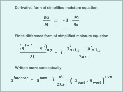
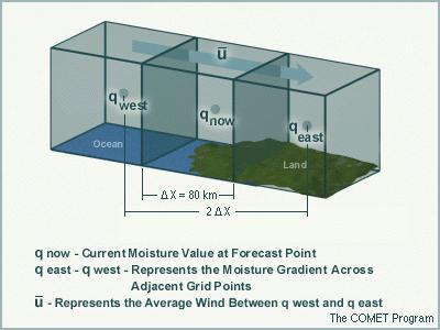
16 7.5 NWP Equations Introduction The PRIMITIVE EQUATIONS are used as the forecast equations in NWP models. Vilhelm Bjerknes first recognized that numerical weather prediction was possible in principle in He proposed that weather prediction could be seen as an initial value problem in mathematics Since equations govern how meteorological variables change with time, if we know the initial condition of the atmosphere, we can solve the equations to obtain new values of those variables at a later time (i.e., make a forecast).

17 To represent an NWP model in its simplest form, we can write: A = t F(A) where A gives the change in a forecast variable at a particular point in space t gives the change in time (how far into the future we are forecasting) F(A) represents terms that can cause changes in the value of A This equation means that the change in forecast variable A during the time period t is equal to the cumulative effects of all processes that force A to change.

18 Future values of meteorological variables are solved for by finding their initial values and then adding the physical forcing that acts on the variables over the time period of the forecast. This is stated as A forecast = A initial + F(A) t where F(A) stands for the combination of all of the kinds of forcing that can occur The process is then repeated for the duration of the simulation This stepwise process represents the configuration of the prediction equations used in NWP.

19

20 7.5.2 Problems associated with NWP equations 1. The way in which primitive equations are derived from their complete theoretical form and converted to computer codes can contribute to errors 2. The model forecast equations are simplified versions of the actual physical laws governing atmospheric processes, especially cloud processes, landatmosphere exchanges, and radiation. The physical and dynamic approximations in these equations limit the phenomena that can be predicted. 3. Due to their complexity, the primitive equations must be solved numerically using algebraic approximations, rather than calculating complete analytic solutions. These numerical approximations introduce error even when the forecast equations completely describe the phenomenon of interest and even if the initial state were perfectly represented.

21 4. Computer translations of the model forecast equations cannot contain all details at all resolutions. Therefore, some information about atmospheric fields will be missing or misrepresented in the model even if perfect observations were available and the initial state of the atmosphere were known exactly. 5. Grid point and spectral methods are techniques for representing information about atmospheric variables in the model and solving the set of forecast equations. Each technique introduces different types of errors.

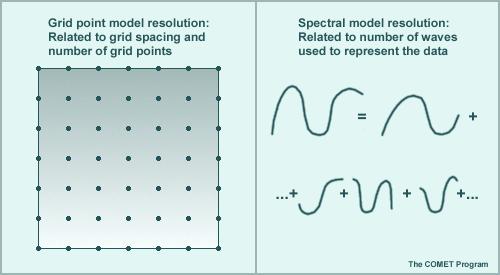
22 7.6 Model Types Introduction The type of model being used (grid point or spectral) influences: 1. How the model equations are solved 2. How the data are represented 3. The type of weather features that can be resolved We will look at 4 different types of models: 1. Grid point models 2. Spectral models 3. Hydrostatic models 4. Non-hydrostatic models

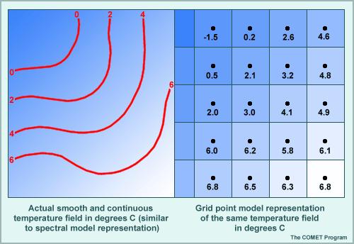
23 7.6.2 Grid Point Models 1) Data Representation In the real atmosphere, wind, pressure, temperature, and moisture vary from location to location in a smooth, continuous way Grid point models, however, perform their calculations on a fixed array of spatially disconnected grid points. The values at the grid points actually represent an area average over a grid box. The continuous temperature field shown in the next graphic, therefore, must be represented at each grid point as shown by the black numbers in the right panel of the previous graphic. The temperature value at the grid point represents the grid box volume average.

24

25 Grid point models actually represent the atmosphere in three-dimensional grid cubes, such as the one shown below. The temperature, pressure, and moisture (T, p, and q), shown in the center of the cube, represent the average conditions throughout the cube. The east-west winds (u) and the north-south winds (v), located at the sides of the cube, represent the average of the wind components between the center of this cube and the center of the adjacent cubes. Similarly, the vertical motion (w) is represented on the upper and lower faces of the cube. This arrangement of variables within and around the grid cube (called a staggered grid) has advantages when calculating derivatives. It is also physically intuitive; average thermodynamic properties inside the grid cube are represented at the center, while the winds on the faces are associated with fluxes into and out of the cube.

26

27 2) Truncation Errors Grid point models must use finite difference techniques to solve the forecast equations. In the real atmosphere, advection often occurs at very small scales. The greater the distance between grid points, the less likely the model will be able to detect small-scale variations in the temperature and moisture fields. The lack of resolution introduces errors into the solution of the finite difference equation. Deficiencies in the ability of the finite difference approximations to calculate gradients and higher order derivatives exactly are called TRUNCATION ERRORS. The examples below show that the use of fewer and more widely spaced grid points reduces the amount of detail and increases the magnitude of errors introduced into the solutions of the model forecast equations

28 1. Urban smog (wavelength ~ 40 km): Only two model grid points describe the wave representing the urban smog. The feature is present but its shape and variations within it are not represented well. Even before the forecast begins, the model's representation of the feature has lost around 25% of the feature's amplitude. A large amount of the gradient is lost near the wave peaks and yet even more of the gradient at the edges of the feature. This small-scale feature is barely contained in the model initial conditions.

29 2. Frontal rain or snow bands (wavelength ~ 80 km): Four model grid points describe the wave representing the frontal rain or snow bands. The presence of the feature is obvious but the shape is poorly represented. If this were a frontal rain band, the cloudy/rainy part of the band and the dry area between bands would be recognizable but the peak intensity would be missed. The feature clearly exists in the model initial conditions but the details are considerably smoothed. This will impact the forecast.

30 3. Mid-tropospheric shortwave (wavelength ~ 400 km): Twenty model grid points describe the wave representing the shortwave. The model representation of this mid-tropospheric shortwave is nearly identical to the data. In the old NCEP Nested Grid Model (NGM), this wave, with a wavelength on the order of 400 km, would span only five model grid points. Therefore, the NGM model representation would only be somewhat better than the frontal precipitation band example shown for a 20-km resolution model

31 Summary Characteristics Data are represented on a fixed set of grid points Resolution is a function of the grid point spacing All calculations are performed at grid points Finite difference approximations are used for solving the derivatives of the model's equations Truncation error is introduced through finite difference approximations of the primitive equations The degree of truncation error is a function of grid spacing and time-step interval

32 Advantages Can provide high horizontal resolution for regional and mesoscale applications Do not need to transform physics calculations to and from gridded space As the physics in operational models becomes more complex, grid point models are becoming computationally competitive with spectral models Non-hydrostatic versions can explicitly forecast details of convection, given sufficient resolution and detail in the initial conditions

33 Disadvantages Finite difference approximations of model equations introduce a significant amount of truncation error Small-scale noise accumulates when equations are integrated for long periods The magnitude of computational errors is generally more than in spectral models of comparable resolution Boundary condition errors can propagate into regional models and affect forecast skill Non-hydrostatic versions cover only very small domains and short forecast periods

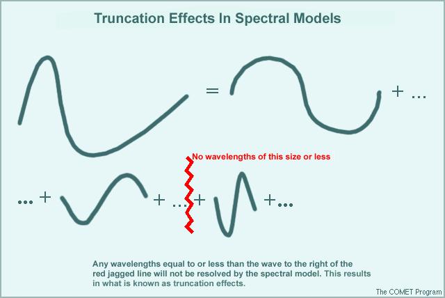
34 7.6.3 Spectral Models 1) Data Representation Spectral models represent the spatial variations of meteorological variables as a finite series of waves of differing wavelengths Consider the example of a hemispheric 500-hPa height field in the top portion of the graphic below. If the height data are tabulated at 40 N latitude every 10 degrees of longitude (represented at each yellow dot on the chart), there are 36 points around the globe. It takes a minimum of five to seven points to reasonably represent a wave and, in this case, five or six waves can be defined with the data. The locations of the wave troughs are shown in the top part as solid red lines.

35 When the data are plotted in the graph, the five wave troughs are definable by the blue dots but are unequally spaced. This indicates the presence of more than one wavelength of small-scale variations. In this case, the shorter waves represent the synopticscale features, while the longer waves represent planetary features.

36 2) Truncation Errors What are the effects of truncation in a spectral model? Recall that in a grid point model, truncation error is associated with the finite difference approximations used to evaluate the derivatives of the model forecast equations. One of the nice features of the spectral formulation is that most horizontal derivatives are calculated directly from the waves and are therefore extremely accurate. This does not mean that spectral models have no truncation effects at all. The degree of truncation for a given spectral model is associated with the scale of the smallest wave represented by the model.

37

38 A grid point model tries to include all scales but does a poor job of handling waves only a few grid points across. A spectral model represents all of the waves that it resolves perfectly but includes no information on smallerscale waves. If the number of waves in the model is small (for example, T80), only larger features can be represented and smaller-scale features observed in the atmosphere will be entirely eliminated from the forecast model. Therefore, spectral models with limited numbers of waves can quickly depart from reality in situations involving rapid growth of initially small-scale features. Several types of wave orientation are possible in spectral models. Triangular (T, as in T170) configuration is the most common in operational models since it has roughly the same resolution in the zonal and meridional directions around the globe.

39 SUMMARY Characteristics Data are represented by wave functions Resolution is a function of the number of waves used in the model Model resolution is limited by the maximum number of waves The linear quantities of the equations of motion can be calculated without introducing computational error Grids are used to perform non-linear and physical calculations Transformations occur between spectral and grid point space Equations can be integrated for large time steps and long periods of time Originally designed for global domains

40 Disadvantages Transformations between spectral and grid point physics calculations introduce errors in the model solution Generally not designed for higher resolution regional and mesoscale applications Computational savings decrease as the physical realism of the model increases Advantages The magnitude of computational errors in dynamics calculations is generally less than in grid point models of comparable resolution Can calculate the linear quantities of the equations of motion exactly At horizontal resolutions typically required for global models (late 1990s), require less computing resources than grid point models with equivalent horizontal resolution and physical processes

41 7.6.4 Hydrostatic Models Most grid point models and all spectral models in the current operational NWP models are hydrostatic. This means that no vertical accelerations are calculated explicitly. The hydrostatic assumption is valid for synoptic- and planetary-scale systems and for some mesoscale phenomena. An important exception is deep convection, where buoyancy becomes an important force. Hydrostatic models account for the effects of convection using statistical parameterizations approximating the larger-scale changes in temperature and moisture caused by non-hydrostatic processes.

42 SUMMARY Characteristics Use the hydrostatic primitive equations, diagnosing vertical motion from predicted horizontal motions Used for forecasting synoptic-scale phenomena, can forecast some mesoscale phenomena Used in both spectral and grid point models (for instance, the AVN/MRF and Eta)

43 Disadvantages Cannot predict vertical accelerations Cannot predict details of small-scale processes associated with buoyancy Advantages Can run fast over limited-area domains, providing forecasts in time for operational use The hydrostatic assumption is valid for many synopticand sub-synoptic-scale phenomena

44 7.6.5 Non-Hydrostatic Models Currently, most non-hydrostatic models are grid point models. They are generally used in forecast or research problems requiring very high horizontal resolution (from tens of meters to a few kilometers) and cover relatively small domains. Non-hydrostatic models can explicitly (directly) forecast the release of buoyancy in the atmosphere and its effects on the development of deep convection. To do this, non-hydrostatic models must include an additional forecast equation that accounts for vertical accelerations and vertical motions directly, rather than determining the vertical motion diagnostically from horizontal divergence.

45 Changes in the vertical motion from one time step to the next in a grid box are caused by: 1. advection bringing in air with a different vertical velocity 2. pressure deviations from hydrostatic balance resulting from changes in horizontal convergence/divergence phenomena with non-hydrostatic pressure perturbations, such as thunderstorms and mountain waves 3. Buoyancy (B): Positive (negative) buoyancy generates a tendency toward upward (downward) motion. Positive buoyancy is caused by warm temperature anomalies in a grid box compared to its surroundings higher moisture content in a grid box compared to its surroundings 4. Downward drag caused by the weight of liquid or frozen cloud water and precipitation

46 To account for vertical motions and buoyancy properly, non-hydrostatic models must include a great deal of detail about cloud and precipitation processes in their temperature and moisture forecast equations. Since hydrostatic models do not have a vertical motion forecast equation, none of these processes can directly affect the vertical motion in their predictions. One disadvantage of non-hydrostatic models is longer computation time. Since the models must finish running in time for forecasters to use model products, hydrostatic models are more advantageous unless non-hydrostatic phenomena need to be simulated or unless resolution finer than around 10 km is needed. Non-hydrostatic models run at very high resolution characteristically predict detailed mesoscale structure and associated forecast impacts on surrounding areas.

47 SUMMARY Characteristics Use the non-hydrostatic primitive equations, directly forecasting vertical motion Used for forecasting small-scale phenomena Predict realistic-looking, detailed mesoscale structure and consistent impact on surrounding weather, resulting in either superior local forecasts or large errors

48 Disadvantages Take longer to run than hydrostatic models with the same resolution and domain size Used for limited-area applications, so they require boundary conditions (BCs) from another model; if the BCs lack the structure and resolution characteristic of fields developing inside the model domain, they may exert great influence on the forecast May predict realistic-looking phenomena, but the timing and placement may be unreliable Advantages Calculate vertical motion explicitly Explicitly predict release of buoyancy Account for cloud and precipitation processes and their contribution to vertical motions Capable of predicting convection and mountain waves

49 7.7 Vertical Coordinates A model's vertical structure is as important as the horizontal structure and model type. To represent the vertical structure of the atmosphere properly requires selection of a suitable vertical coordinate and sufficient vertical resolution. Unlike the horizontal structure of models where discrete or continuous (grid point or spectral) configurations can be used, virtually all operational models use discrete vertical structures. As such, they produce forecasts for the average over an atmospheric layer between the vertical-coordinate surfaces, not on the surfaces themselves.

50 7.7.1 Sigma Vertical Coordinate The equations of motion have their simplest form in pressure coordinates. Unfortunately, pressure coordinate systems are not particularly suited to solving the forecast equations because, like height surfaces, they can intersect mountains and consequently 'disappear' over parts of the forecast domain. To deal with this problem Phillips (1957) developed a terrain-following coordinate called the sigma (σ) coordinate. The sigma coordinate or variants are used in the NGM, GFS, ECMWF, NOGAPS, and UKMET models and appear in some mesoscale models, such as MM5, COAMPS, and RAMS.

51 The sigma coordinate is defined by σ = p/p s, where p is the pressure on a forecast level within the model and p s is the pressure at the earth's surface, not mean sea level pressure. The lowest coordinate surface (usually labeled σ = 1) follows a smoothed version of the actual terrain. Note that the terrain slopes used in sigma models are always smoothed to some degree. The other sigma surfaces gradually transition from being nearly parallel to the smoothed terrain at the bottom of the model (σ = 1) to being nearly horizontal to the constant pressure surface at the top of the model (σ = 0). The sigma vertical coordinate can also be formulated with respect to height (z), rather than pressure.

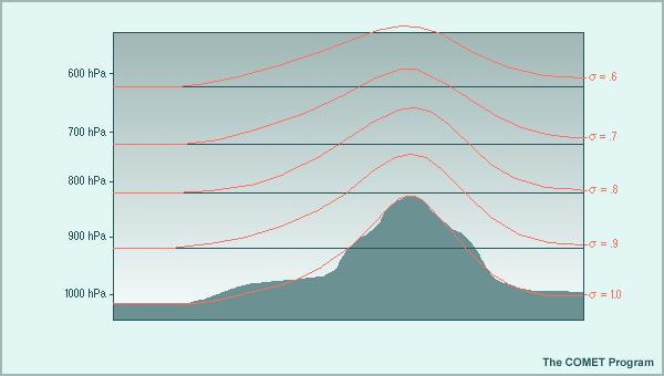
52

53 7.7.2 Eta Vertical Coordinate The eta coordinate (η ) was created in the early 1980s in an effort to reduce the errors incurred in calculating the pressure gradient force using sigma coordinate models. The eta coordinate is, in fact, another form of the sigma coordinate, but uses mean sea level pressure instead of surface pressure as a bottom reference level. As such, eta is defined as where η p t is pressure at the model top s p = p r ( ) r zs pt ( z = 0) pt p r (z=0) is the standard atmosphere MSL pressure (1013 hpa) p r (z s ) is the standard atmosphere pressure at the model terrain level z s

54 η s = p p r ( ) r zs pt ( z = 0) pt

55 Calculating Eta Surfaces First, the heights at each model level must be defined. In this example, we have defined a model with 10 eta layers (only 3 shown) distributed evenly with respect to pressure from sea level to the top of the atmosphere. Standard atmosphere pressures are then determined at each of these heights. At point 1, the actual terrain elevation is 848m. This is closest to the 1000-m height defined for the first eta level. The standard atmosphere pressure at that height is 900 hpa. What, then, is the eta level closest to this point? Using the eta equation, η = (900-0) / (1000-0) =.9 If we go to point 2, the actual terrain height is 1126 m and is also closest to the 1000-m height. Therefore, the eta level closest to this point is again.9. However, if we go up to point 3 (1832 m), the nearest eta surface in the model is at 2000 m. Here the standard atmospheric pressure is 800 hpa. The nearest eta level is therefore = 1 x (800-0 / ) =.8. Note that the eta levels are predefined and the model topography is set to the nearest eta surface even if it does not quite match the average or smoothed terrain height in the grid box. This has been a simplified example. In reality, it is necessary to choose the intervals between eta levels in a way that both depicts the planetary boundary layer (PBL) with sufficient detail and yet represents the average changes in elevation over the entire forecast domain.

56 Eta usually is labeled from 0 to 1 from the top of the model domain to mean sea level. Some of the model's grid cubes are located underground in areas where the surface elevation is notably above sea level. This requires special numerical formulations to model flow near the earth's surface. The Eta coordinate systems allows the bottom atmospheric layer of the model to be represented within each grid box as a flat "step," rather than sloping like sigma in steep terrain. This configuration eliminates nearly all errors in the PGF calculation and allows models using the eta coordinate to have extreme differences in elevation from one grid point to its neighbor.

57 Eta coordinate models can therefore develop strong vertical motions in areas of steep terrain and thus more accurately represent many of the blocking effects that mountains can have on stable air masses. Even when the step-like Eta is used as the vertical coordinate, model terrain is still much coarser than real terrain, but the topographic gradients are less smoothed than in sigma models. Note that the Eta levels are predefined and the model topography is set to the nearest eta surface even if it does not quite match the average or smoothed terrain height in the grid box.

58 Sigma vs Eta Surfaces

59 Advantages of the Eta Coordinate 1. Eta models do not need to perform the vertical interpolations that are necessary to calculate the PGF in sigma models. 2. Although the numerical formulation near the surface is more complex, the low-level convergence in areas of steep terrain are more representative of real atmospheric conditions than in the simpler formulations in sigma models. 3. Compared with sigma models, Eta models can often improve forecasts of cold air outbreaks, damming events, and leeside cyclogenesis For example, in cold-air damming events, the inversion in the real atmosphere above the cold air mass are preserved almost exactly in an eta model. As a result, there is little or no contribution to erroneous horizontal temperature gradients in the lee of the mountains

60 Therefore, the model channels the flow over the mountains above and parallel to the cold air inversion, rather than producing erroneous downslope flow. The improvement in the depiction of downslope flow also results in more realistic "vortex-tube stretching" (and thus more accurate increases in vorticity) in leeside cyclogenesis events.

61 Limitations of the Eta Vertical Coordinate 1. The step nature of the eta coordinate makes it difficult to retain detailed vertical structure in the boundary layer over the entire model domain, particularly over elevated terrain 2. Eta models do not accurately depict gradually sloping terrain. 3. Eta models have difficulty predicting extreme downslope wind events. 4. Eta models must broaden valleys a few grid boxes across or fill them in. 5. Eta coordinates can create spurious waves at step edges.

62 7.7.3 Isentropic Vertical Coordinate Since flow in the free atmosphere is predominantly isentropic, potential temperature (θ ) can be very useful as a vertical coordinate system. However, non-adiabatic processes dominate in the boundary layer and isentropic surfaces intersect the earth's surface. For these reasons, potential temperature alone is not currently used as a vertical coordinate in any operational numerical model system. However, isentropic coordinates do form an essential part of many hybrid vertical coordinate systems.

63 Advantages of Isentropic Coordinates 1. The theta coordinate allows for more vertical resolution in the vicinity of baroclinic regions, such as fronts, and near the tropopause. 2. For adiabatic motion, air flows along constant theta (isentropic) surfaces and implicitly includes both horizontal and vertical displacement. 3. Vertical motion through isentropic surfaces is caused almost exclusively by diabatic heating. The vertical component of the isentropic forecast equations is related entirely to diabatic processes. 4. Isentropic coordinate models conserve important dynamical quantities, such as potential vorticity.

64 Limitations of Isentropic Coordinates 1. Isentropic surfaces intersect the ground. 2. Isentropic coordinates may not exhibit monotonic behavior with height, especially in the boundary layer. Superadiabatic layers can develop anywhere in the atmosphere, but predominantly occur in the boundary layer due to diurnal heating. When they develop, isentropic surfaces then appear more than once in the vertical profile above a point, something that cannot be allowed in a model's vertical coordinate system. 3. Vertical resolution in nearly adiabatic layers is coarse. 4. Isentropic surfaces have steep slopes in the vicinity of sharp baroclinic regions, such as fronts which can produce inaccuracies in the horizontal pressure gradient.

65 7.7.4 Hybrid Vertical Coordinates Different hybrid combinations are currently in use, eg: hybrid isentropic-sigma vertical coordinates, hybrid sigma-pressure coordinate, hybrid isentropic-sigma coordinate Hybrid isentropic-sigma coordinate models have a combination of sigma layers at the bottom that shift to isentropic layers above. Uniting theta and sigma into one vertical coordinate system combines the terrain-following advantages of sigma and the increased vertical resolution in key baroclinic areas due to the adaptive nature of isentropic surfaces.

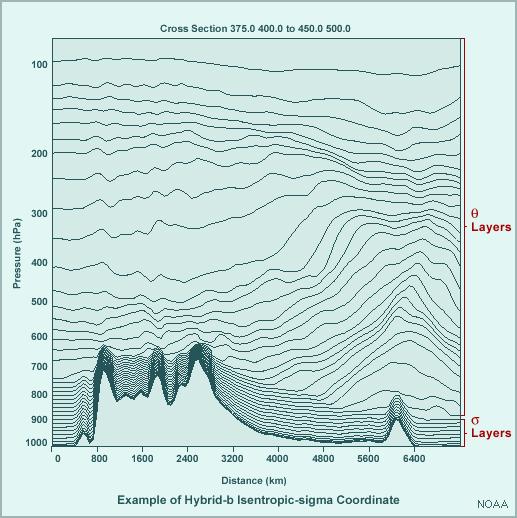
66

67 7.7.5 Special Considerations for Non- Hydrostatic Models The requirement that non-hydrostatic models solve a prognostic vertical motion equation constrains the choice of vertical coordinate and increases computation time, which competes with horizontal and vertical resolution for limited computational resources. The result is that Most non-hydrostatic models use a vertical coordinate based on height. (A few are pressure-based, and none use isentropic coordinates.) Most non-hydrostatic forecast models sacrifice vertical resolution in order to run the models in real time at fine horizontal resolution. The ratio of vertical to horizontal resolution is typically poor. This inconsistency can introduce numerical noise into the forecast

68 7.7.6 Summary: Vertical Coordinate Systems Vertical Coordinate Models Primary Advantage Primary Limitation Eta Eta Allows for large local differences in May not represent the boundary layer Boundary layer at low elevations terrain from one with sufficient Regions of steep grid point to resolution over surface slopes another elevated terrain Other targeted levels (jet stream) Generic Hybrid Isentropic Sigma Hybrid Sigma ECMWF, NOGAPS RUC AVN/MR F, NGM, MM5, RAMS Combines strengths of several coordinate systems Naturally increases resolution in baroclinic regions, such as fronts and tropopause Surfaces are terrain following and therefore resolve the boundary layer well Difficult to properly interface across coordinate domains Incompletely depicts important low-level adiabatic flow May not correctly portray weather events in the lee of mountains Well Simulated Atmos Layers Varies based on hybrid Boundary layer Baroclinic features in free atmosphere Tropopause Boundary layer Other targeted levels (jet stream)

69 7.8 Horizontal Resolution The horizontal resolution of an NWP model is related to the spacing between grid points for grid point models or the number of waves that can be resolved for spectral models. RESOLUTION' is defined here in terms of the grid spacing or wave number and represents the average area depicted by each grid point in a grid point model or the number of waves used in a spectral model. Note that the smallest features that can be accurately represented by a model are many times larger than the grid 'resolution.' In fact, phenomena with dimensions on the same scale as the grid spacing are unlikely to be depicted or predicted within a model.

70

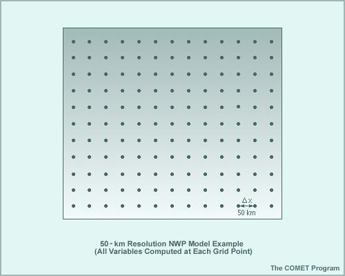
71 7.8.1 Grid Spacing A grid point model s horizontal resolution is defined as the average distance between adjacent grid points with the same variables. For example, if all of a model's forecast variables (u-wind, v- wind, temperature, and moisture, etc.) are predicted at each of its grid points (as shown in the next slide), the model is considered to have a resolution equal to the minimum spacing between adjacent grid points at a specific latitude and longitude, which in this case is 50 km. A similar model with 10 km between adjacent grid points is considered to have 10-km horizontal resolution.

72

73 Whether a model is considered high or low resolution depends upon the size of the domain and the scale of weather phenomenon that the model is trying to predict. A resolution on the order of 20 to 50 km is considered high for a global model, while for a storm-scale model, a resolution of 100 to 500 m is considered high and necessary to resolve the internal processes of convection. Resolution (high or low) is a relative term and changes with the development of new models and increasing computer power It is important to know the amount of area between grid points, since atmospheric processes and events occurring over areas near to or smaller than this size will not be included in the model.

74 For a 50-km model (in the next slide), each grid box covers 2500 square kilometers, with the grid points located at the center of the boxes. Hence, the central "grid point" represents the mean value of the data within the 2500 square kilometer area of the grid box surrounding the "grid point. The grid point is assigned a value of 26, which approximates the average of the observed values within the grid box. This representation may be adequate when the area is under a rather homogeneous, large-scale feature, such as a large high-pressure system. However, if the scale of the phenomena being forecast is less than the area represented by the grid box, the phenomena will not be correctly represented and can, if not treated properly, actually degrade the quality of forecasts of large-scale features.

75 Grid spacing also has direct and indirect effects on Model terrain representation Truncation errors in equation computations Computer resources A model's ability to resolve different scales of features

76 7.8.2 Spectral to Grid Point Resolution Equivalency In spectral models, the horizontal resolution is designated by a "T" number (for example, T80), which indicates the number of waves used to represent the data. The "T" stands for triangular truncation, which indicates the particular set of waves used by a spectral model. Spectral models represent data precisely out to a maximum number of waves, but omit all, more detailed information contained in smaller waves. The wavelength of the smallest wave in a spectral model is represented as minimum wavelength = 360 degrees N where N is the total number of waves (the "T" number).

77 Complications arise because non-linear dynamics and physics are calculated on a grid and then converted to spectral form to incorporate their effects in a spectral model. This introduces errors, which make the final result less exact than one might expect from calculations done strictly in spectral space. Spectral models do a fine job with 'dry' waves in the free atmosphere, but have coarser representation of the physics, including surface properties. The resulting overall forecast quality is somewhere between these two extremes and varies on a case-by-case basis. The more physics that is involved in the evolution of the forecast, the less the advantage in spectral model forecasts compared to comparable resolution grid point forecasts.

78 7.8.3 Representing Terrain Terrain representation in numerical models is usually much smoother than in reality, especially in coarse resolution models. Terrain smoothing is largely a function of a model's horizontal resolution and the detail of the topographic dataset. Terrain smoothing can be a large source of error in regions affected by small-scale orographic features. Several methods are used to convert terrain height data to model orography in order to get a representative terrain value for each model grid box

79 Mean orography uses the average of the terrain data inside a model grid box. This trims the tops of mountains considerably, especially if the grid box is large, greatly diminishing the blocking effect on cross-mountain flow. Envelope orography is like a blanket over the terrain that clings to plateaus but rises smoothly to cover all but the very sharpest peaks. This ensures that the full effect of terrain blocking and lee side cyclogenesis can be simulated. However, the valleys are filled and the terrain is considerably smoothed.. Silhouette orography averages only the tallest features in each grid box. Thus, it lies below the mountaintops but above the valleys. The NCEP Eta Model uses a variation of silhouette orography that enables more detail of valleys.

80 Two factors limit model representation of orography: The horizontal resolution of the model The horizontal resolution of the terrain dataset used If the terrain dataset is coarse, it cannot provide details about the topography to high-resolution models. If the model cannot resolve terrain features, terrain details provided in the dataset will be averaged out. In most cases, some terrain smoothing is desirable, in part because airflow over complex terrain otherwise generates small-scale noise that can mask the largerscale signal. To get more accurate forecasts for precipitation location and amounts, both the model and the topographic dataset used by the model must be of high resolution. On the next slide, a heavy precipitation event in the L.A. basin, illustrates the effects of increased resolution and better-resolved topography.

81 The top panels show precipitation forecasts from the 29-km and 10-km Eta models, the bottom panel the observed precipitation. The 10-km Eta has better resolved topography, as reflected in the improved placement of the precipitation, especially for heavier amounts. In addition, the precipitation amounts forecast by the 10-km Eta are closer to observed values.

82 Model terrain can affect the following: Vertical motion fields are shifted away from the mountains Precipitation maxima and minima are misplaced or missing in regions of complex terrain. Downslope winds, valley winds, drainage winds, and other small-scale processes typically cannot be depicted The propagation speeds of near-surface frontal zones are impacted Mountain wave development often cannot be accurately depicted Valley inversions and cold air damming are often difficult to resolve and are not well represented Note that the vertical coordinate and vertical resolution also strongly impact the nature of terrain effects.

83 7.8.4 Land/Water Interface Considerations Models also have difficulty resolving features influenced or caused by the interface between land and large bodies of water. Since the properties of land and water are so different, a model will do a poor job of representing the processes that occur or are influenced by land/water interfaces if its resolution is not sufficient to determine their location. The example shows why models with insufficient resolution do a poor job of defining such features and processes as sea and lake breezes/fronts, lake-effect snow bands, and coastal fronts

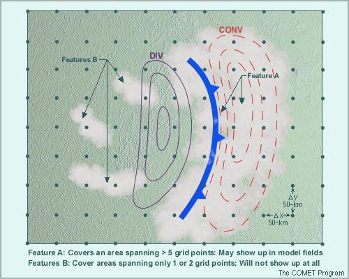
84 7.8.5 Feature Resolution Introduction A model's ability to resolve meteorological features on different scales depends upon a number of factors: 1. Grid spacing or number of waves (horizontal resolution) 2. Available computer resources 3. Model terrain representation 4. Amount of truncation error that will occur within a model's primitive equations Models tend to have the greatest difficulty resolving features influenced or caused by characteristics of the earth's surface that are not adequately represented in the model, such as terrain and coastal interfaces, and with small-scale features, such as MCSs and outflow boundaries.

85 It typically takes at least five grid points to define a feature in a grid point model. The smallest scale phenomena that can be preserved, even within short-range forecasts, have wavelengths of five to seven grid point spacings. Phenomena that can be preserved in one- to two-day forecasts typically have wavelengths greater than eight to ten grid spaces. In the example of a convergence/divergence couplet (next slide) associated with a cold front, a grid point model with 50-km resolution cannot be expected to resolve the smaller features (Features B). The larger frontal feature, associated convergent region, and cloud mass (Feature A) will show up in the model fields. Features smaller than 250 km but greater than 50 km may be seen by the model but will not be adequately resolved, leading to errors in the model's depiction of the feature's characteristics. Note that even if a feature meets the resolvable size criteria, it may still be inadequately resolved based on its orientation and juxtaposition within the model grid.

86

87 7.8.6 Summary: Grid Point and Spectral Models Grid Point Models Horizontal resolution is defined as the distance between grid points The smallest features that can be forecast in a grid point model should have full wavelengths of five to seven grid points Computer resources limit how small a model's grid spacing can be, given the large increase in computing time required to run higher-resolution models Grid spacing affects a model's ability to represent terrain, which, in turn, affects how well the model can define terrain-induced or terrain-enhanced meteorological phenomena Grid spacing impacts the amount of truncation error (degree of error associated with the computation of model primitive equations), which introduces increasing amounts of error to the primitive equation calculations as they are carried out over time

88 Spectral Models Horizontal resolution is a function of wave number (number of waves used to represent the data) Higher numbers (more waves) indicate finer resolution The more waves used to represent the data, the more computing power required to carry out the calculations Terrain representation and associated weather are improved when the number of waves is increased Truncation is a function of the wave number and refers to the minimum wavelength used by the model to represent the data. Smaller wavelengths are truncated and are not used in the calculations A model's ability to resolve features depends not only on its horizontal resolution, but also on its vertical resolution, number of vertical layers, and the physics package used to define a variety of surface and atmospheric processes. Additionally, limited-area models are strongly constrained by their boundary conditions.

89 7.9 Vertical Resolution Adequate vertical resolution, like horizontal resolution, is important Virtually all operational models use discrete vertical structures. The ratio of the horizontal and vertical resolutions must be consistent with the slope of the weather phenomena of interest. The vertical coordinate systems have different abilities to represent weather features in the vertical based on their vertical resolution characteristics. In all vertical coordinate systems, layer thickness must change gradually from one layer to the next. Since resolution must be a few tens of meters near the ground to properly depict a variety of surface processes, there must be a large number of levels in the PBL layer to act as a transition zone with the less-closely spaced levels in the mid-troposphere

90 7.9.1 Vertical Resolution Requirements The vertical resolution of operational models must be sufficient enough to: 1. Incorporate the effects of diurnal heating and cooling 2. Incorporate local effects of spatially variable surface characteristics 3. Depict flow and shear in the boundary layer 4. Capture ageostrophic regimes associated with uppertropospheric jet streaks 5. Detect interactions between the stratosphere and troposphere, including multiple high-level jets 6. Monitor stratospheric regimes that affect medium-range forecasts and trace gas concentrations

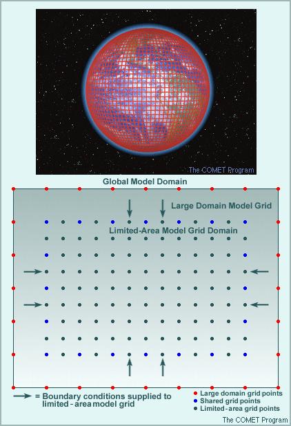
91 7.10 Domain and Boundary Conditions MODEL DOMAIN refers to a model's area of coverage. LIMITED-AREA MODELS (LAMs) have horizontal (lateral) and top and bottom (vertical) boundaries GLOBAL MODELS cover the entire earth and have only vertical boundaries. For limited-area models, larger-domain models supply the data for the lateral boundary conditions.

92

93 For all models, accurate information must be provided for all forecast variables and along each model boundary (lateral, top, and bottom) in order to solve the forecast equations. Boundary values can be obtained from a variety of sources, including: Data assimilation systems Forecast values from a current or previous cycle of a large-scale model (as is the case for lateral boundary conditions used in LAMs) Some type of climatological or fixed value (for specifying certain surface characteristics, such as soil moisture, sea surface temperature, and vegetation type)

94 Lateral Boundaries The lateral boundary conditions largely control the position and evolution of features that cover the entire forecast domain. For example, for a domain covering the 48 states, longwave patterns are almost entirely determined by the boundary conditions. Weaker impacts are noted on jet streaks and fronts, especially in regions far downwind from the upstream boundary. Similarly, in a high-resolution mesoscale model running over a small section of the country, the placement and timing of synoptic-scale features are determined almost completely by the synoptic-scale model supplying the boundary conditions.

95 The animation in the next slide shows how far an air parcel can travel into a limited-area model domain from the model boundary during a 48-hr forecast period. Since the influence of boundary conditions spreads away from (and particularly downstream of) the boundaries and, in some cases, the effects amplify downstream, the area of primary forecast concern should be located as far from the boundaries as possible, especially the upstream boundary.

96

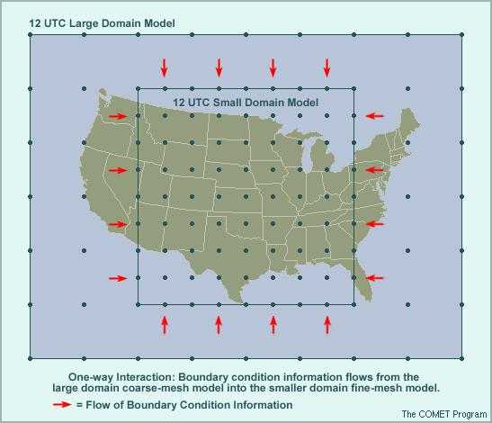
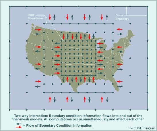
97 Treatment of Lateral Boundaries One-way interaction: Information flows in one direction, from the coarser-mesh, larger domain to the finer-mesh, smaller domain. Computations within the finer-mesh model do not affect the larger domain model. Two-way interaction: Information flows in both directions in the interior grid interfaces of a nested model. The coarser-grid forecast supplies boundary conditions to the finer-grid forecast, while the finer-grid forecast is used by the coarser grid in determining the forecast variables.

98

99

100 Two-way interaction is highly advantageous for several reasons: It allows fine-scale processes resolved on the fine mesh to affect the larger-scale flow on the coarse mesh. For instance, a large convective system resolved on the fine mesh can amplify an upper ridge, slowing the progression of waves in the westerlies in the larger-domain coarse resolution grid. Because predictions on coarse-resolution grids take relatively little computer time and memory resources, the outermost boundary of the model can be moved far from the region of forecast interest, while the fine-resolution domain remains small enough to run in real time. The use of these "real-time" boundary condition procedures within a model with the same basic forecast dynamics and physics greatly reduces the influence of errors associated with using boundary conditions from a model with older data and a different vertical coordinate, topography, and physics.

101 Top and Lower Boundary Conditions Top boundary conditions are treated well enough in most models to be of little concern to forecasters The lower boundary interfaces with the model representation of surface processes. Failure to realistically represent all relevant physical processes or accurately describe the physical state of the ground generates error in the model forecast. Lateral boundary conditions and lower boundary specifications are major sources of model forecast error.

102 7.11 Sources of Model Error Three categories of model errors: 1. Errors in initial conditions 2. Errors in the model 3. Intrinsic predictability limitations

103 Errors in Initial Conditions Inadequate spatial density Inadequate temporal frequency Instrument error/data transmission problems Representativeness errors Quality control errors Objective analysis errors (weighting and interpolation) Data assimilation difficulties

104 Errors in the Model Incomplete formulation of equations of motion Horizontal and vertical numerical approximation errors Time interpolation errors Boundary conditions (only vertical in global models) Inadequate terrain representation Large-scale precipitation processes not well estimated Shortcomings of convective parameterizations Estimations of clouds and cloud radiative processes Heat, moisture, and momentum flux approximations (both between ground and air, & BL and free atmosphere)

105 Intrinsic Predictability Limitations Unmeasured scales of motion (energy transfer between scales) Error growth with time

106 7.12 Model Clouds and Precipitation In predicting precipitation in NWP models we need to differentiate between resolvable (grid-scale) and parameterized (sub-grid scale) processes Operational models do not currently explicitly resolve and predict convection - convection needs to be parameterized in these models Precipitation and cloud parameterization (PCP) schemes need to be linked to convective parameterization (CP) schemes to simulate the precipitation process As model resolution and complexity continue to increase, convection and convective precipitation can be treated together through interactions between the model dynamics and the PCP scheme. CP is no longer required since its purpose is to represent the effects of convection when those effects could not be produced explicitly.

107 Some Definitions Precipitation and cloud parameterization (PCP): refers to the model emulation of cloud and precipitation processes that remove excess atmospheric moisture directly resulting from the dynamically driven forecast wind, temperature, and moisture fields. PCP schemes have commonly been referred to as grid-scale precipitation schemes. Convective parameterization (CP): is the method by which models account for convective effects through the redistribution of temperature and moisture in a grid column, which reduces atmospheric instability. By reducing thermodynamic instability, CP prevents the grid-scale PCP scheme from creating unrealistic largescale convection and overly active low-level cyclogenesis.

108 Generating Clouds and Precipitation

109 While grid-scale motions determine the forcing, additional cloud and precipitation processes occurring at scales much smaller than a grid box also influence the true microphysical response -> these need to be parameterized Sub-grid scale response due to PCP includes: latent heating due to condensation which affects the wind, temperature, and moisture fields. evaporative cooling associated with precipitation in subsaturated layers These feedbacks may further strengthen the circulation that initially produced the model clouds and precipitation. The strengthened circulation may increase the precipitation and latent heating, which, in turn, may result in additional feedbacks.

110 Types of Schemes Traditionally, PCP schemes have been based solely on the prediction of relative humidity (RH). They infer the presence of clouds in grid layers based upon RH saturation thresholds and immediately condense all excess moisture into precipitation. Recent improvements to PCP schemes include predicted cloud water. These schemes range from simple schemes that account for cloud water only to more complex schemes that include many types of hydrometeors and internal cloud processes.

111 Schemes Using Inferred Clouds Description: These are schemes that infer precipitation to remove excess moisture and infer clouds, all based on RH. Models: The AVN/MRF, NGM, and NOGAPS models use inferred cloud schemes. Process of removing grid-scale moisture: Areas of excess moisture or supersaturation must be present in the sounding to diagnose precipitation. (Note that the effects of ice or phase changes are not accounted for) In these schemes: all water in the atmosphere remains in vapor form ->RH is too high, because no water is held in cloud precipitation falls out instantaneously

112 Initial State Post- Precipitation State

113 Strengths Run fast Simple and easily understood Driven by the relatively well-forecast wind, temperature, and moisture fields Perform acceptably in low-resolution models since the schemes do not account for small-scale motions Limitations Not physically realistic Data assimilation systems cannot incorporate cloud data All precipitation must fall out of the grid column in one timestep The precipitation rate is an average for a grid box

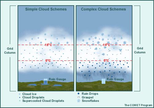
114 Introduction to Cloud Schemes Schemes using predicted clouds follow a physically based sequence of forming clouds prior to precipitation. Schemes using simple clouds diagnose precipitation from cloud water (or ice) only. Schemes using complex clouds predict precipitation directly through the modeling of internal cloud processes, including multiple cloud and precipitation hydrometeor types.

115

116 Schemes Using Simple Clouds Description: These are schemes that predict cloud water/ice based on RH and then infer or diagnose precipitation based on cloud water/ice amount. Models: The Eta Model uses a simple cloud scheme. In these schemes: resulting RH is more realistic because some water and ice is condensed in clouds; not all is held in vapor form as in inferred cloud schemes precipitation falls out instantaneously

117 Initial State Cloud State

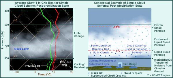
118 Postprecipitation state

119 Strengths Improvement in precipitation amount and location over inferred cloud schemes because: clouds can be advected the effects of cloud ice on precipitation processes can be included RH fields are more realistic since some water and/or ice is held in clouds Direct comparisons of model initial and forecast cloud fields with satellite imagery Assimilation of cloud data to improve moisture fields since cloud water is a predicted variable Improved radiation processes distinguishing between cloud water and ice improves the simulation of radiative effects of water versus ice clouds Are better suited for higher-resolution models because more microphysics details and smaller-scale motions can be taken into account

120 Limitations More computationally expensive Improvements in precipitation forecast are not complete because Precipitation is still a byproduct, rather than predicted directly, and falls to the ground in one time step Precipitation hydrometeors are not explicitly predicted The precipitation rate is an average for a grid box which can lead to over or under forecasts of precipitation by the model depending upon the actual extent and rate of the precipitation In reality, precipitation rates may vary considerably at individual points within a grid-box area In reality, sub grid-scale variability in precipitation amount increases as the grid-box area increases Microphysics are too simple to be able to predict convective processes, such as the creation of cold pools and gust fronts

121 Schemes Using Complex Clouds Description: These are schemes that predict clouds and precipitation based on RH by directly predicting precipitation hydrometeors and accounting for internal cloud processes. These schemes are only used in higher-resolution models because they require sufficient model resolution to resolve small-scale variability affecting microphysical processes. Models: The RUC and AFWA MM5 use schemes with complex clouds (cloud liquid, cloud ice, rain, snow, graupel), and research models like RAMS (cloud water, pristine ice, rain, snow, aggregates, graupel and hail) In this scheme: precipitation is tracked as it falls to the ground, rather than falling to the ground instantaneously. some water or ice remains held in clouds, making the resulting environmental RH more realistic

122 Initial State Cloud State

123 Precipitation begins Precipitation reaches ground

124 Strengths Models can directly predict precipitation type reaching the surface and amounts of each type Can directly predict cooling from evaporating and/or melting precipitation Can realistically predict snow to blow far downwind from regions where it is generated Can depict convective system anvil extent and stratiform rain region Development and areal coverage of cirrus anvils is improved. (This is important because of the effect of ice clouds on radiation in the atmosphere) Cloud cover and areal coverage/duration of precipitation from a convective system is improved through the inclusion of multiple major hydrometeors

125 Assimilation of remote sensing data is further improved Can include satellite-derived information on some hydrometeor types Can incorporate radar data into the assimilation process Can verify forecast precipitation type using surface observations Can directly forecast aircraft icing based on the existence of supercooled water in clouds and precipitation Environmental RH fields are more realistic because some water or ice is held in clouds Since more hydrometeor types are accounted for, the radiation scheme is further improved over simple cloud schemes

126 Limitations Can become prohibitively expensive (in model run time and memory requirements) to implement Require sufficient model resolution to resolve small-scale variability affecting microphysical processes. Can be difficult to determine which cloud hydrometeors are most important for different situations and applications, such as aircraft icing Although cloud data can be used in data assimilation systems, direct measurements of hydrometeor types and concentrations are not normally available Data for verifying hydrometeor concentrations do not exist for the full depth of observed cloud Because data for initial concentrations of cloud and precipitation hydrometeors are typically not available, the PCP scheme has to "spin up" until equilibrium is reached between the hydrometeors and the forecast moisture, temperature, and wind fields. This results in the underprediction of clouds and precipitation early in the forecast

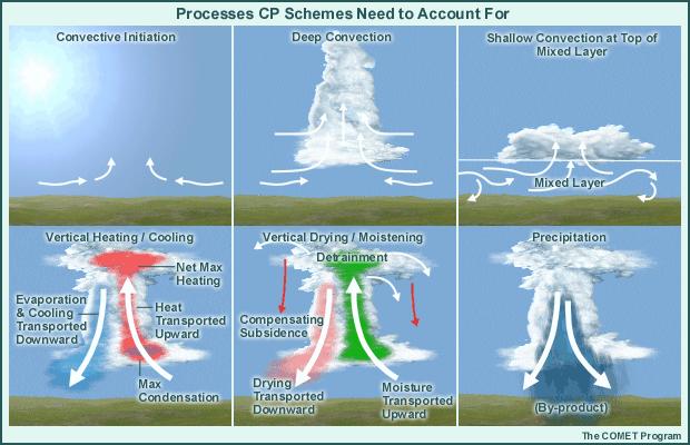
127 7.13 Convective Parameterization In nature, convection serves not only to produce precipitation, but also to transport heat upward, redistribute moisture, and thereby stabilize the atmosphere. If enough convection occurs over a large enough area, it can also create outflow jets and mid-level vortices and drive larger atmospheric circulations that affect weather in distant locations, etc. Models must try to account for these types of convective effects. Given the scale at which convective processes occur, though, current operational models cannot predict them explicitly and must do so via parameterization.

128 What is Convective Parameterization Cumulus or convective parameterization schemes are procedures that attempt to account for the collective influence of small-scale convective processes on largescale model variables All NWP models with grid spacing larger than that of individual thunderstorms or storm clusters need to parameterize the effect that convection has on largerscale model variables in each grid box Why is Convective Parameterization Important? Convective storms can significantly influence vertical stability and large-scale flow patterns by Redistributing heat, moisture, and momentum Producing cloud cover that affects surface temperatures

129

130 Convective parameterization schemes are primarily designed to account for the vertical transport of latent heat, which drives the general circulation in the tropics reduce thermodynamic instability so the grid-scale precipitation and cloud parameterization (PCP) schemes do not try to create unrealistic large-scale convection and overly active low-level cyclogenesis. CP schemes reduce instability by rearranging temperature and moisture in a grid column

131 Formulation of Convective Parameterizations No matter how they are formulated, all convective parameterization schemes must answer these key questions: 1 How does the large-scale weather pattern control the initiation, location, and intensity of convection? 2 How does convection modify the environment? 3 What are the properties of parameterized clouds? Each scheme must define the following, using information averaged over entire grid boxes: 1. What triggers convection in a grid column 2. How convection, when present, modifies the sounding in the grid column 3. How convection and grid-scale dynamics affect each other

132 Convection Initiation and Intensity Schemes can initiate convection by considering the Presence of some convective instability at a grid point (perturbed parcels may reach LFC) Existence of low-level and/or vertically-integrated mass/moisture convergence that exceeds some threshold at a grid point Rate of destabilization by the environment at a grid point Schemes can make the intensity of the convection Proportional to the moisture or mass convergence or flux Sufficient to offset the large-scale destabilization rate Sufficient to eliminate the CAPE (this is constrained by the available moisture)

133 Convective Feedback In the real atmosphere, convection modifies the largescale thermodynamics via detrainment (creates large-scale evaporative cooling and moistening) subsidence in the ambient environment (creates large-scale warming and drying) When a model changes the vertical temperature and moisture profiles as a result of convective processes, it is referred to as convective feedback The issue for convective parameterization schemes used in any given model is how they determine the new vertical distribution of heating, cooling, moistening and/or drying caused once convection is triggered

134 Two Approaches to Convective Feedback Adjustment Schemes Simulate the effects of convection by adjusting the lapse rates of both temperature and moisture to a directly specified empirical reference profile at each grid point (without attempting to simulate the explicit convective process) Make the profile a function of the difference between the moist adiabat inside the cloud and the moist adiabat representative of the ambient environment Convective adjustment schemes are generally best suited for large-scale models and for situations requiring less intensive computational resources Mass Flux Schemes DO attempt to explicitly model convective feedback processes at each grid point

135 The mass flux schemes DO attempt to explicitly formulate and account for convective processes at each grid point. This is accomplished by combining a cloud model with the assumption that convection acts to restore the grid column to a stratification based on moist parcel stability. The cloud model estimates the properties of the convection and the closure assumption specifies the amount of convection that occurs in order to achieve the desired rate of stabilization. While the mass flux approach is more physically consistent than the empirical adjustment approach, it does have its tradeoffs as well. Because they are more complex, mass flux schemes introduce new problems that require the schemes to make additional assumptions.

136 Convective Parameterization Schemes There are numerous different convective parameterization schemes. Some of the more well-known schemes currently used in operation models include: 1. Kuo Scheme 2. Betts-Miller-Janjic Scheme 3. Arakawa-Schubert Scheme 4. Kain-Fritsch Scheme

137 1) Kuo Scheme Description: This is a simple scheme that produces precipitation and increases static stability by emulating the moist-adiabatic ascent of a parcel. It adjusts the temperature and moisture profiles toward moist adiabatic. Models: The Kuo Scheme is used in the NGM and is an option in many research and local models

138 2) Betts-Miller-Janjic Scheme Description: This scheme is slightly more complex than the Kuo scheme. It adjusts the sounding toward a predetermined, post-convective reference profile derived from climatology. Models: The BMJ scheme is used in the operational NCEP Eta Model.

139 3) Arakawa-Schubert Scheme Description: This is a complex scheme. It includes the effects of moisture detrainment from convective clouds, warming from environmental subsidence, and convective stabilization in balance with the large-scale destabilization rate. Models: Variations of the Arakawa-Schubert scheme are used in the AVN/MRF, the NCEP Regional Spectral Model, and the RUC as well as some climate and research models.

140 4) Kain-Fritsch Scheme Description: This is a complex scheme designed to rearrange mass in a column so that CAPE is consumed. Models: The Kain-Fritsch scheme is used in the NSSL Experimental Eta Model. It may also be used in some members of the NCEP short-range ensemble in the future. In addition, it is an option in some research and local models.

141 Convective Parameterizations in the Various Operational Numerical Models Notice that mesoscale models are not restricted to any one particular parameterization scheme and may implement some of the schemes listed to the right, other schemes, or none at all.

142 Explicit Convection High-resolution (1-2 km) non-hydrostatic models (eg RAMS, MM5, ARPS) can be run without CP schemes because the grid spacing is small enough to begin resolving convective motion The model dynamics and the PCP scheme results in: explicitly simulated updrafts strong enough to lift hydrometeors up to the equilibrium level explicitly simulated downdrafts and their accompanying gust fronts

143 This allows a more realistic redistribution of heat and moisture than when a CP scheme is used. It also enables the winds and vertical motion to be modified directly by the convection. Explicit convection ultimately provides a direct prediction of convective precipitation. In storm-scale models (< 2 km), all precipitation can be calculated "explicitly ; no convective parameterization is necessary (although microphysical processes are still parameterized)

144 The animation shows how the experimental non-hydrostatic ARPS model uses explicit convection to realistically simulate the 3 May 1999 OKC tornadic supercells as compared to radar observations of the same storms.

145 7.14 Model Comparisons We will now briefly examine the details of 3 of the most commonly used operational models: 1. the ETA model 2. the Global Forecast System (GFS) model which includes the Medium Range Forecast Model (MRF) and a Global Data Assimilation System (GDAS) 3. the Rapid Update Cycle (RUC) model, the research counterpart of which is the Mesoscale Analysis and Prediction System (MAPS) For more information on these models or their characteristics you can look at: We will also look at a mesoscale / cloud scale research / forecast model: 1. Regional Atmospheric Modeling System (RAMS)

146 Current Common Operational Models Model Fundamentals ETA GFS RUC Model Type Grid point Spectral Grid point Vertical Coordinate System Horizontal Resolution Eta Sigma Hybrid Isentropic-Sigma 12 km T km Vertical Resolution 60 layers 64 layers 50 layers Domain Regional Global Regional Precipitation and Cloud Schemes Convective Parameterization Schemes Predicted Total Condensate Betts-Miller- Janic Simple Cloud Simplified Arakawa- Schubert EXMOISG Complex Cloud Scheme Grell/Devenyi Ensemble Cumulus Parameterization

147 Model Fundamentals Atmospheric Radiation Cloud and Radiation ETA GFS RUC Clear-Sky Radiative Transfer Diagnosed Cloud Water and RH Clouds Water Surfaces OMB 2D- VAR SST Snow Ice NESDIS Snow Cover, USAF Snow Depth NESDIC Ice Analysis Chou SW, RRTM LW Diagnosed Cloud water and RD Clouds Reynolds SST NESDIS Snow Cover, USAF Snow Depth NESDIS Ice Analysis CO2 and Water Vapor Dudhia Cloud / Radiation Scheme OMB 2D-VAR SST 2-Layer Snow model

148 Model Fundamentals Vegetation Type and Vegetation Fraction Soil Type and Soil Moisture Turbulence ETA GFS RUC GCIP Vegetation Type, NESDIS Vegetation Fraction 4-Layer Pan-Mahrt Soil Model Mellor- Yamada 2.5 Level Closure GCIP Vegetation Type, NESDIS Vegetation Fraction 2-Layer Soil Model First-Order, Non-Local (Pan and Mahrt) 24 Vegetation Classes 6-Layer soil model Burk and Thompson

149 ETA Model Domain

150 GFS Domain

151 RUC Domain

152 RAMS RAMS Basic Characteristics Regional Atmospheric Modeling System (RAMS) Grid point model Two-way interactive nested grids Sigma-z vertical coordinate Horizontal resolution: various tremendously from 100s meters to 100s kilometers Vertical resolution: varies tremendously Domain: LES to semi-hemispheric Sophisticated microphysics: Single- and two-moment microphysics; 7 hydrometeor species (cloud water, rain, pristine ice, snow, aggregates, graupel and hail) Convective Parameterizations: Kain-Fritsch, Kuo Radiation: several different schemes Surface: LEAF2 model, 11 or more soil levels Turbulence: Mellor-Yamada, Smagorinsky

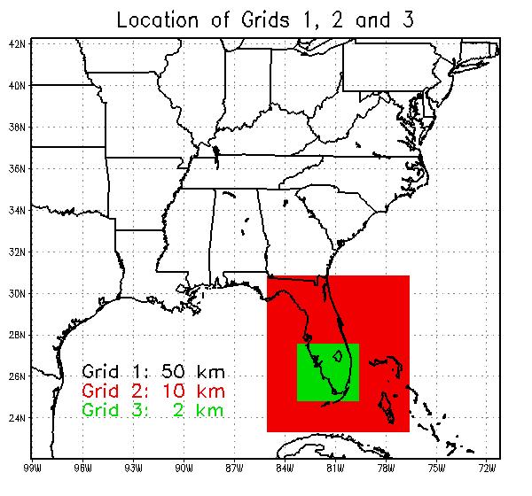
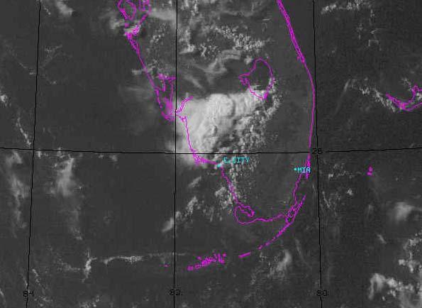
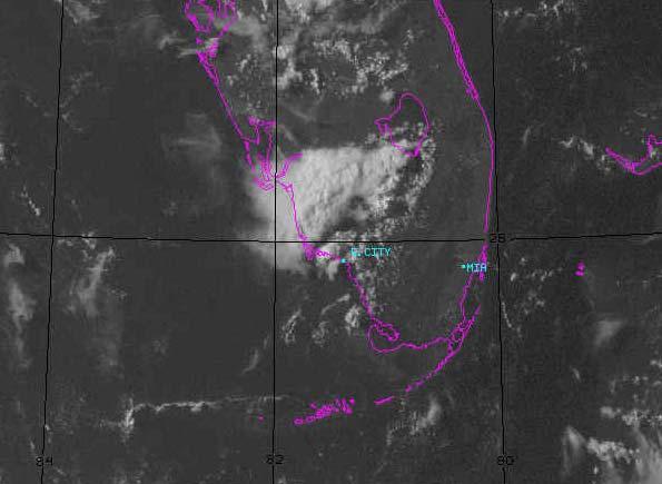
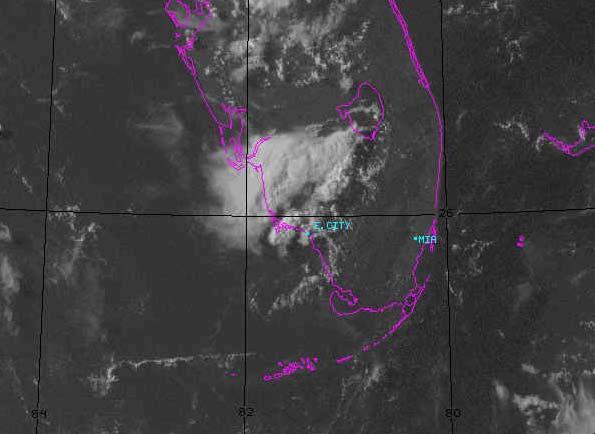
153 RAMS Simulation Example The Cirrus Regional Study of Tropical Anvils and Cirrus Layers Florida Area Cirrus Experiment (CRYSTAL-FACE) July 2002 Florida peninsula and surrounding oceans Case Study: 28 July 2002 Easterly wave over the southern regions of the Florida peninsula Storms along W coast in the regions of Everglade City, Fort Meyers, and Tampa Presence of Saharan dust

154 Source: NASA LaRC

155

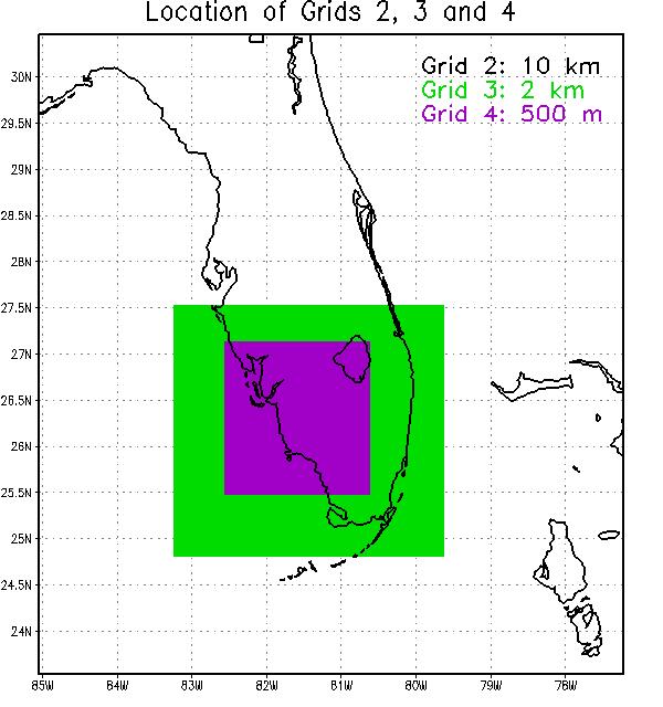
156 Model Setup Details 4 grids Horizontal grid spacing: Grid 1: x = y = 50 km Grid 2: x = y = 10 km Grid 3: x = y = 2 km Grid 4: x = y = 500 m Vertical grid spacing: 36 levels Stretched 8 levels within first 1km AGL Initialized at 12Z with 40 km Eta data Simulation run for 12 hours Two-moment microphysics Microphysical species: cloud water, rain, pristine ice, snow, aggregates, graupel, hail Other microphysical aspects: second cloud mode, CCN and GCC Sophisticated vegetation and soil model 40 vegetation classes (USGS) allows for standing water

157

158

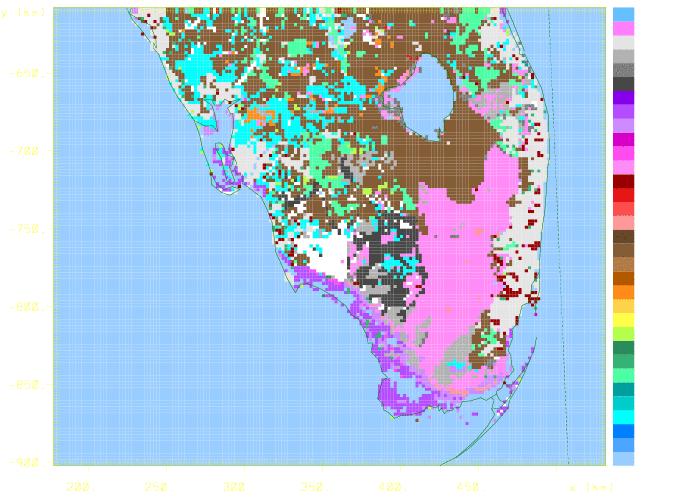
159 Grid 3 Vegetation

160 700 mb geopotential heights (color), wind speed (white contours, m/s) and wind vectors after 12 hours of simulation time (00z on 07/29) Corresponding 700 mb analysis

161 Vertical velocity (red, isosurface: 1m/s)

162 Vertical velocity (red, isosurface 1m/s) and pristine ice (yellow, isosurface 0.3 g/kg)

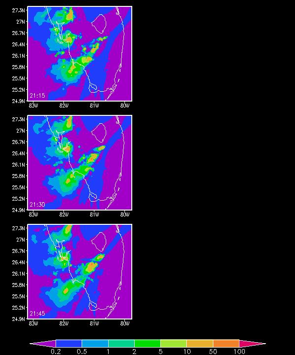
163 Vertically integrated condensate (mm) and visible satellite imagery

164 Vertical velocity (red, 1m/s), pristine ice (yellow, 0.3 g/kg), hail (green, 1g/kg), rain (mauve, 1g/kg), graupel (orange, 1g/kg) and cloud water (blue, 0.3 g/kg)