Use of Geophysical Software for Interpretation of Ice-Penetrating Radar Data and Mapping of Polar Ice Sheets

Transcription

1 Use of Geophysical Software for Interpretation of Ice-Penetrating Radar Data and Mapping of Polar Ice Sheets Alex O. Martinez University of Kansas 2335 Irving Hill Road Lawrence, KS Technical Report CReSIS TR 102 July 28, 2006 This work was supported by a grant from the National Science Foundation (#ANT ).

2 Introduction The effects of global warming in our world are going to have a significant impact on human activities in the future. The rising temperature in our atmosphere can cause climate changes, including melting of most of the glaciers around the world, which will cause a rise in sea level. Scientists are studying the impact of global warming on glaciers and ice sheets in Greenland and Antarctica. The University of Kansas has been performing research in Greenland and Antarctica using radar depth sounder systems to measure the thickness of ice sheets. Knowing the ice thickness is important because we can use it to calculate the mass balance of the ice sheets and their possible contribution to sea level rise if they are reduced. Therefore, efficient and accurate determination of ice thickness from the radar data offers the means to understand the behavior of ice sheets and their potential impact on sea level and climate. In this work we test the use of exploration geophysics software for interpretation of airborne radar data acquired by the University of Kansas. For the project we used the December 6, 2002, data set acquired by the Improved Coherent Antarctic and Artic Radar Depth Sounder (ICARDS). These data required processing and re-formatting in order to import them to the seismic-interpretation software Kingdom Suite. For these processes we implemented the use of MatLab. This work resulted in maps of the ice surface, base reflectors, and an isochron/isopach map representing ice thickness. 2

3 Objectives of this Project The objective of this project is to develop methods for the use of geophysical software to interpret airborne radar data collected over polar ice sheets. Software such as SMT Kingdom Suite allows users to visualize digital data in 3D, interpret horizons (layers) in the data, and generate maps. Such capabilities can facilitate interpretation of large data sets such as the ones acquired by CReSIS. Methodology Radar data sets available from prior University of Kansas field seasons were tested in this work. We used the December 6, 2002, data acquired by the Improved Coherent Antarctic and Artic Radar Depth Sounder (ICARDS). This project is divided into two different procedures: the first involves the implementation of MatLab software and the second one uses Kingdom Suite. MatLab was important for processing and reformatting, and Kingdom Suite was for interpretation of the data. Data Reformatting and Conversion to SEG-Y We obtained the data from CReSIS in their original format and converted them to SEG-Y format using MatLab. SEG-Y is the data formatting standard used in seismic exploration; therefore, the radar data needed to be converted to SEG-Y in order to use the seismic interpretation software Kingdom Suite. This program was very important to this project because it offers the capability to interpret large digital data sets; MatLab also is a very helpful tool to analyze seismic data. To change the radar data to SEG-Y format, we used the SEGY Mat script made by Thomas Mejer Hansen from the University of 3

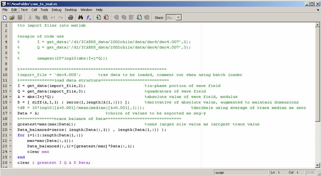
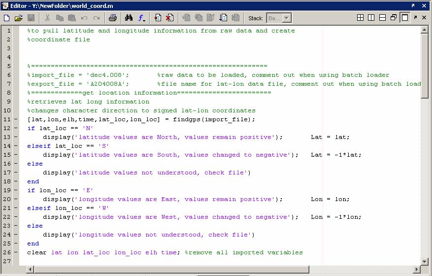
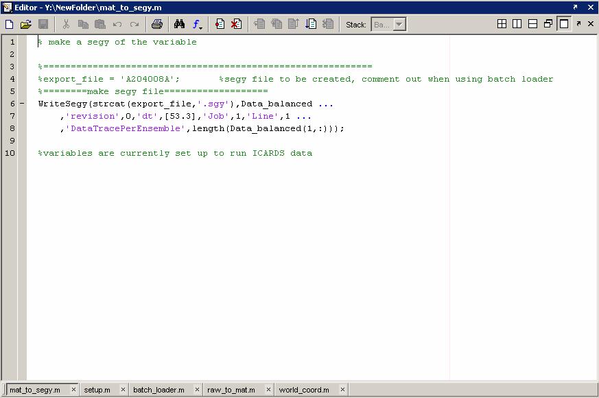
4 Copenhagen in Denmark. This script is a set of m-files that helps import and export SEG- Y files from MatLab. We employed a two-step method: the first is to acquire the radar data and the second to acquire the location of these data. We made several scripts (Appendix A) in order to accomplish this task, and each script had a different assignment. Scripts used were in this order: setup.m: with this script we can choose the location where MatLab is going to import and export data. batch_loader.m is used for implementing the commands for importing raw files and exporting location data. raw_to_mat.m was created to choose which part of the data we want to use. This way we can import the real and imaginary values of the data, as well as calculate and import the absolute value of the wave field, the derivative of absolute value and the decibel information. This script was useful to decide which type of information was the best to use and study. world_coordinate.m was useful to write the location information and export to another file. This location is in the format of latitude and longitude and can be read in Kingdom Suite. Location of fight paths is very important to this study, because we want to know exactly where the radar was transmitting and receiving information so we can know exactly where the structures inside the ice are located. mat_to_segy.m functions to write SEG-Y files. 4

5 In this project we used the absolute value, the derivative, and the decibel magnitude of the ICARDS data in order to determine which data type was suitable for interpretation in Kingdom Suite. After all location files for each SEG-Y file were written, we imported them into Kingdom Suite for visualization and interpretation. Data Visualization and Interpretation Kingdom Suite is seismic interpretation geophysical software used by geoscientists to map the subsurface. The purpose for using this software is to test the idea that it can be used to interpret airborne radar data from the Center for Remote Sensing of Ice Sheets (CReSIS). The steps for visualization of this data are simple, beginning with loading the SEG-Y files into Kingdom Suite. This process took time because the whole data set comprised 63 files and we had to load them one by one. Then the files that contain the location description were loaded separately; each SEG-Y file must have one location file associated with it. The complete description of how to load these files can be found in Appendix B. This software provided us the ability to load a base map of Antarctica (Figure 1a) and position the radar survey accurately in the map (Figure 1b). This way we can represent graphically in space where the structures in the ice sheets are located. To display the survey lines in the map, we adjusted the coordinate system to Universal Polar Stereographic Coordinate System and used the South Zone system. 5

6 Area of study Figure 1a. Map of Antarctica imported to the interpretation software. 6

7 December 6, 2002 flight survey Figure 1b. Base map showing the survey, which consists of 63 lines. Each data transect can be seen as a two-dimensional image where y axis is time and x axis is trace number. The spatial position of each trace is specified by the location file. This representation is convenient since we are able to recognize different structures like the surface of the glacier, the bedrock underneath, and some layers inside the ice sheet (see Figures 2, 3 and 4). 7

8 Amplitude Time (µs) Ice Surface Reflection Figure 2. Time vs. Trace Number graph displaying the absolute value of the magnitude of the ICARDS December 6, 2002, Antarctica data set. X and Y locations are listed at the lower-left corner of the window. Am plitude Time (µs) Ice Bed Reflection Figure 3. Time vs. Trace Number graph displaying the derivative of the absolute values shown in Figure 2. 8

9 Amplitude Time (µs) Internal Structures Ice Bed Reflection Figure 4. Time vs. Trace Number graph displaying the data of figure 2 in decibel scale. A stronger bed reflection is identifiable in this data form. The y axis represents the time that the wave traveled in (µs), while the x axis is the trace numbers. This picture shows the arrival times of the electromagnetic wave; the first arrival is the direct arrival from the transmitter antenna to the receiver antenna, then the surface of the ice appears very clearly and some internal layers are apparent. Below the surface a strong pulse can be seen in most of the files; this is a multiple return created by the wave reflecting from the ice surface and the aircraft. This picture also shows a very weak signal reflected off the ice bed; this possibly could be because of the attenuation of the signal as it travels through ice. In some files, the ice bed reflector tends to be weaker as the ice grows thicker. 9

10 In each file we picked 4 different horizons: for example, in Figure 5 we can see the direct arrival (orange), ice surface (green), first multiple (pink) and ice bed (black). Direct arrival Surface of Ice First multiple Ice Bed Figure 5. Example of the file Dec6-003_D After all horizons were picked, we constructed maps of the surface and ice bed horizons. These horizons were used to construct an isochron map where we can see the changes in ice thickness. 10

11 Interpretation The horizons picked in each file were helpful in constructing a map along the survey line and displaying in two dimensions the arrival times of each horizon. Time (µs) Effect due to changing altitude No Data Horizon: Ice Surface Antarctica December 6, 2002 Figure 6. Ice Surface Horizon The horizon shown in Figure 6 is the surface horizon picked in every data file. This horizon is relatively smooth and there are no big changes in the time. Most of the survey shows low values, but the first 3 files and the final 3 files change very rapidly because the aircraft that made the survey is at first higher in altitude, then descends at a lower altitude during most of the flight until it takes off again to higher altitudes in the end. This effect can be eliminated by correcting the data for aircraft altitude changes. We did not apply such correction in this work. In some areas the radar was unable to acquire 11

12 good data; as a result these areas have no color in the surveyed line because it was impossible to pick any horizon. The same procedure was repeated with the ice bed horizon. Figure 7 illustrates the survey line with the picked ice bed horizon. The bed reflector appears deeper in the green areas and shallower in the white-yellow areas. Note that the first three and last three files are strongly affected by aircraft altitude changes, similar to the ice surface horizon. Time (µs) Horizon: Ice Bed Antarctica December 6, 2002 Figure 7. Ice Bed Horizon 12

13 After picking horizons, we produced data grids that allowed us to comprehend more about the surface by using interpolating procedures; for this we used Inverse Distance to a Power method of interpolation. The most accurate values in these grids are the ones closer to the line of survey, and the areas that are far away are less reliable because there is no information nearby to be interpolated by the software. The grid of the surface of the ice is shown in Figure 8; this grid shows the surface more or less constant through the survey line, while the effect of the change in altitude of the aircraft can be seen in the upper-left corner of the grid. Time (µs) Grid of Ice Surface Antarctica December 6, 2002 Figure 8. Grid of Surface. 13

14 In Figure 9, the grid of the ice bed is illustrated. This grid shows how the topography changes at the base of the ice sheet. If we had more survey lines in this map the grid would be more accurate. Aircraft altitude changes are also seen in the upper-left corner of the grid. Time (µs) Grid of Ice Bed Antarctica December 6, 2002 Figure 9. Grid of Ice Bed 14

15 The grid isochron in Figure 10 represents the two-way travel time difference between the ice surface and ice bed reflectors. Using an average electromagnetic wave velocity in ice of 0.16 m/ns yields an estimate of ice sheet thickness (isopach). Yellow and red represent the thicker areas of the ice sheet. Blue represents less thick ice, and pale colors show thinner ice. This observation fits with the fact that this area is on the ice shelf on the coast. 2-Way Time (µs) Thickness (m) Grid: Isochron Antarctica December 6, 2002 Figure 10. Grid Isochron and Isopach 15

16 3D Visualization The visualization of the data in Kingdom Suite was prepared without difficulty. For this project we selected an intersection where two lines converge (Figure 11). The lines loaded were lines 11 to 14 and 46 to 44 in orthogonal direction. Three-dimensional visualization is the best aspect for viewing ice sheets because it assists in the understanding of the geomorphology of the bed rock. Since CReSIS studies ice sheets over a period of time, 3D pictures can be an excellent tool to visualize internal layers and ice bed changes. Area of 3D Visualization Figure 11. Base map Antarctica showing survey line and the area of threedimensional visualization. 16

17 Figure 12 is an example of how lines are arranged in space. In this image we can observe the ice surface horizon on top and ice bed horizon on the bottom. The vertical axis represents time; therefore, this image does not demonstrate true thickness. To calculate true thickness we must find the velocity function of the wave traveling through ice. This type of problem is not solved in this project; however, we can perceive in this 3D image how long the wave travels through the boundaries between air and ice surface and ice and bedrock. Ice Surface Horizon Ice Bed Horizon Figure 12. Radar data with surface and ice bed horizon in a 3D representation. 17

18 With all the information of horizons and grids, we could put together a 3D display. In Figure 13, we loaded the radar lines displaying the decibel scale. To these lines we loaded the bedrock horizon and surface horizon and then the ice surface grid. The final result is a three-dimensional display of the ice sheet. Ice Surface Grid Ice Bed Horizon Figure 13. 3D Visualization of Ice Surface and Ice Bed 18

19 Results We accomplished our objectives in this project: we developed a methodology for importing (ICARDS) airborne radar data into a seismic data processing and visualization software. MatLab was used for processing and reformatting the radar data. Data converted to SEG-Y format were imported into Kingdom Suite. The implementation of Kingdom Suite software for interpretation of radar data was successful and brings new capabilities to ice sheet studies. Because of the versatility in this software we had the opportunity to work with large data volumes. We interpreted surface and base reflectors of the West Antarctic Ice Sheet image from the December 6, 2002, survey and created an isochron/isopach map of ice thickness. Acknowledgments I would like to thank the Center for Remote Sensing of Ice Sheets for giving me the opportunity to work on this project as an undergraduate researcher. I also thank Anthony Hoch for his help in this work and Professor George Tsoflias for support in this project. 19

20 Appendix A This appendix is a list of MatLab scripts used in this project for importing and writing SEG-Y format files. setup.m batch_loader.m 20

21 raw_to_mat.m world_coordinate.m 21

22 mat_to_segy.m 22

23 Appendix B This appendix show different steps for visualizing radar data. Kingdom Suite This program allows us to understand and analyze the data. Open the Kingdom Suite program, then choose 2d/3d Pack from the menu. In the main window, click on the project icon bar, then choose create new project. Then select the file you want to open. In the next window, select any project database (in this work we used MS Access 2003). In the Project Options window, select OK. In the next window, select no so the program won t search for an existing coordinate system. 23

24 In the main menu, select the survey tab and Import SEG-Y Files. In the next window, select the first option where it says Import SEGY Files into Single 2D or 3D Survey and click next. Then browse for the correct SEG-Y file in your folders and click next. 24

25 This next window is for selecting the seismic data. If you want to create a new data type, write in the name and select next. In the next window, write the name of the survey and click next. In this window the user has the opportunity to enter the world coordinates, but this time we are going to skip this step by pressing no. In the next window, choose Load Trace Number by Counting and click next. 25

26 In the next window, select Trace Sequence by Counting and click next. In this next window, select IBM Float because the files are set in this format. Click next. Then click finish. 26

27 This is an example of the imported file Dec6-000_D. To import the coordinates, click on the Survey tab and browse by file; in the next window, select which type of information is needed in the file. 27

28 Select the file which contains the coordinate information. Click OK to import coordinates in Feet. In this window, you can select the information you need in the file by clicking on the boxes in the list below. The first column is the shot point (green), the second column is latitude (blue), and the third is longitude (red). After selecting these columns, click OK. 28

29 In the next window select yes to define Project Coordinate System. The next step is to define the coordinate system. In the tab that says Other Coordinate System, select the Universal Polar Stereographic Coordinate System and chose UPS North Zone (if you are working with Greenland data) or UPS South Zone (if you are working with Antarctica data). Then click Define New Coordinate System. 29

30 Click Edit Parameters and change False Northing and False Easting to (0) and change the scale factor to ( ). This factor is the scale factor of the satellite map. Then click OK. 30

31 This is an example of the base map. To import a base map of Antarctica, we downloaded satellite maps from First click on Culture, then choose import, and then look for the image in your directory and open it. Then the image will display in a new window 31