Danish Climate Centre DMI, Ministry of Transport

Transcription

1 Danish Climate Centre DMI, Ministry of Transport The effect of sea surface temperatures on the climate in the extratropics Ph.D. thesis Sannie Thorsen Danish Meteorological Institute & Niels Bohr Institute for Astronomy, Physics and Geophysics Faculty of Science, University of Copenhagen Report 04-01

2 The effect of sea surface temperatures on the climate in the extratropics Danish Climate Centre, Report No Ph.D. thesis, Sannie Thorsen Danish Meteorological Institute & Niels Bohr Institute for Astronomy, Physics and Geophysics Faculty of Science, University of Copenhagen ISSN: X (Print) ISSN: (Online) ISBN: Danish Meteorological Institute, 2004 Danish Meteorological Institute Lyngbyvej 100 DK-2100 Copenhagen Ø Denmark Phone: Fax:

3 Front page Illustration: The atmospheric response in January to an extratropical North Atlantic SST anomaly. The maximum magnitude of the SST anomaly is 2.7 K. The atmospheric response is shown as the average anomalous geopotential height at 500hPa in the last 15 days of the month. Each color level shows an increase or decrease of 10 meters. The 90% confidence level is indicated by one thick black contour and the 95% confidence level is indicated by the second thick black contour. See chapter 2 for a description of the experiment.

4

5 Abstract: The predictability of Europe's climate of a monthly or longer time range is the main topic of the present thesis. The focus is on the fraction of the climate variability which originates from oceanic forcing and the pattern of the atmospheric response. Model simulations are used for the study. The predictive skill of a model is found and possible reasons for a too low predictive skill and methods of improving the skill in models are investigated. The model studies are divided into three main subjects and are each presented in a chapter. The first experiment uses an idealized extratropical sea surface temperature anomaly and the response on a timescale of one month is investigated. The sensitivity of the response to different months climatologies and the size and pattern of the response are found. In the second experiment a model is forced with observed sea surface temperature anomalies and the response in the atmospheric variability on years to decades is found. The 'potential predictability' of the model on different timescales is investigated. The potential predictability is the fraction of the model's atmospheric variance which is forced by the sea surface temperature anomalies. In the third study the climatology of a model is improved by an empirical method. The two versions of the model are compared in order to find the change in predictive skill connected to the improved climatology. In another experiment the sensitivity of the response to a small alteration of the climatology of a model is found on a seasonal timescale. The main results of the studies of monthly and seasonal timescales are: Preferred response patterns of the model determine the position and pattern of the response to SST-anomalies. These preferred response patterns may be in remote areas compared to the position of the extratropical SST-anomalies. Averaging over a season with changing background flow and thereby also changing response patterns is not the reason why the atmospheric response to SST-anomalies is small. The response is still weak when the timescale is of one month or less. In the European area only weak responses are seen to North Atlantic SST anomalies. The main results of the experiments of years to decadal timescale are: A weak but significant potential predictability exists in the extratropics. In the European area significant potential predictability (approximately 20%) exists. The fraction of the SST induced variance compared to the total variance in the atmosphere increases on decadal timescales. This is the case for both the Tropics and the extratropics. A significant part of the North Atlantic Oscillation's variance is predictable in the spring. The model's predictive skill of the NAO is not connected to the El Niño. The correlation coefficients between model simulations and the observed temperatures above Europe are high (40%) in winter and spring. A significant predictability of MSLP exists above Eastern Europe in the fall. A surprising result is that the predictive skill of the model estimated by

6 comparison to observations is higher for Europe than should be expected from the potential predictability estimations. The main results of the experiment of a model with improved climatology are: Improving the climatology of a model does not necessarily improve the predictability in the extratropics. In particular a better representation of the North Atlantic stormtrack did not lead to a better predictive skill above Europe.

7 Table of Contents 1 Introduction Atmospheric sensitivity to sea surface temperature anomalies Predictability The North Atlantic stormtrack and the North Atlantic Oscillation The relation between the atmospheric variance and the ocean AMIP-type experiments The predictability of SST anomalies Evidence of seasonal predictability from observational data for the North Atlantic Evidence of extended predictability from model experiments for the North Atlantic The theory of the atmospheric response to extratropical SST anomalies The midlatitude stormtracks Rossby waves The heat fluxes between ocean and atmosphere Simple theory of the local response of the extratropical atmosphere to anomalous heat fluxes Eddy feedback in GCMs Preferred regimes and response patterns Remote response Summary A model experiment with an idealized North Atlantic SST anomaly The experimental design The SST anomaly The model runs The results Latent and sensible surface heat fluxes The temperature and vorticity response The stormtrack response Local response in geopotential height Probability density function Upper tropospheric zonal wind and wave train crossing the Equator Teleconnected effects in geopotential height Precipitation Discussion Conclusion A model experiment forced by observed SST anomalies The PREDICATE project The setup of the experiment Weaknesses of the experimental design The potential predictability (PP) calculation Results

8 The SST forced variability at different frequencies Zonal average of PP in the pressure fields The Tropics The extratropics The spatial distribution of PP for the pressure fields The Tropics The North Atlantic European region Zonal PP of 2 meter temperature The Tropics The extratropics The spatial distribution of PP for 2 meter temperature The Tropics The extratropics Zonal PP of total precipitation The spatial distribution of PP of precipitation Zonal PP of 10 meter wind squared The spatial distribution of PP of 10 meter square wind The NAO in ECHAM Correlation analysis Power spectrum of the NAO El Niño signal in the NAO Predictive skill in the North Atlantic-European region MSLP The 2 meter temperature Discussion The pressure field The NAO in ECHAM Predictive skill of the ECHAM4 in the North Atlantic European region Conclusion Potential Predictability ECHAM4 predictive skill The NAO MSLP and 2 meter temperature Empirically corrected AGCM The predictability from a corrected version of the ARPEGE model The nudging technique The climatology of the corrected model The predictive skill of the corrected model A second experiment to investigate the predictive skill of a corrected model The difference in response to an North Atlantic SST anomaly in a corrected and an unmodified version of the ECHAM Climatology of the corrected model (DEM) Model simulations of the response to a North Atlantic SST anomaly pattern...108

9 4.3.3 Results Geopotential height response pattern at 500 hpa Response pattern in precipitation Response pattern in 2 meter temperature Conclusion Comparison with results obtained in the experiment from chapter Summary and comparison of results Sensitivity to the background flow (first group of questions) Global response to extratropical SST anomalies Predictability at years to decadal timescales (second group of questions) The predictability in the North Atlantic The gain of predictive skill by improvements of a models climatology (third group of questions) Sensitivity to the background flow, preferred response patterns and remote responses conclusion Acknowledgment References Appendix Mathematical technique to estimate the importance of SST anomalies for the atmospheric variation in a climate model The SST induced variance Frequency dependent SST induced variance Significance testing Ensemble forecast The AGCMs used in the experiments ECHAM The climatology of the ECHAM4.5 and the ARPEGE version

10

11 1 Introduction The original motivation for the thesis was an interest in the possibility of extended range forecasts for Europe. The time range of the predictability could be monthly or seasonally or even as an average at decadal timescale. A necessity for predicting the atmospheric climate variability is an understanding of the interaction between ocean and atmosphere. In this thesis the focus is on the influence of ocean temperature anomalies on the extratropical Northern Hemisphere, in particular the influence of extratropical North Atlantic sea surface temperature (SST) anomalies. The approach to the subject is by model experiments with atmospheric general circulation models (AGCMs) forced by prescribed SST anomalies. The experimental work in the thesis is divided into three parts. The first part focuses on the 'short' timescale. An idealized extratropical SST anomaly is introduced in the North Atlantic and the response during the next month is analyzed using an AGCM. This experiment is described in chapter 2. The second part focuses on timescales between two years and two decades. An AGCM is forced with observed global SSTs, and the result is analyzed to isolate the influence of the SST forcing on the atmospheric variance. This experiment is described in chapter 3. The third part is described in chapter 4. Two experiments investigate how a change in model climatology influences the atmospheric response to SST anomalies. I have only participated in a small part of the work with the experiments of chapter Atmospheric sensitivity to sea surface temperature anomalies The present chapter 1 is mainly a literature survey. The first section discusses predictability in general terms including the difference between the Tropics and the extratropics. The next section describes the North Atlantic Oscillation (NAO). The predictability of the NAO is of high interest for Europe, and the NAO index has often been used in the study of the oceanic influence on the atmosphere. The third section describes the relation between the ocean and the atmospheric variance and discusses the importance of the coupling between ocean models and AGCMs for a predictive skill of atmospheric variability in extended timescales. However, stand alone AGCM experiments are useful for many application and in the fourth section is the special type of model setup called AMIP described. The AMIP experiments are AGCM simulations forced with prescribed SSTs and the limitation and usefulness of this model design are described. This section is included, since several results from this type of setup are discussed in the PhD and the experiment in chapter 3 is of this type. The fifth section discusses the predictability of the SSTs in the extratropics. The predictability of SSTs is a necessity before an extended forecast based on the response of the atmosphere to SSTs can be made. It is shown that indications of an extended predictability of SST anomalies in the extratropics exist. The problem is not further addressed in the experiments of this thesis, since the focus is on the atmospheric response to SST anomalies. In the two next sections (section 6 and 7) experiments 11

12 12 with evidence of seasonal predictions from observational data is discussed and also the evidence for extended forecasts from global circulation models (GCM). Hereafter, the theory for the atmospheric response to extratropical SST anomalies is introduced. These sections are included in order to give a background for the analysis and conclusions made from the experiments later in the thesis. A short introduction to the atmospheric dynamics of the midlatitudes is given in three sections: The midlatitude stormtracks, Rossby waves and the heat flux from the ocean to the atmosphere. In the next section some simple considerations regarding how the atmosphere responds to the heat fluxes are given, and this is followed by more complex considerations. Among those are the role of eddy feedback and preferred atmospheric regimes and response patterns Predictability The predictive skill of climate in a region depends on both the dynamics of the atmosphere, which determine the effect of a known forcing, and on the ability of the numerical model to simulate the dynamics. A model may only have a predictive skill at an extended time range, if both the forcing of the atmosphere and the atmospheric response are known. A simple example of high predictive skill gained from a known forcing is the seasonal variations of the climate. The solar forcing represents a stable varying impact on the climate through the year creating a predictability that can be simulated in statistical as well as dynamical models. However, it is the anomalies relative to the known seasonal average that are usually of interest. A certain predictive skill exists from the initial state of the atmosphere, both through statistical models and through atmospheric general circulation models (AGCM). Statistics show a persistence of the weather anomalies from day to day and also from month to month depending on the season and the geographical area (Fletcher and Saunders 2003). The AGCMs have a predictability of a few weeks using only knowledge of the initial state of the atmosphere (Wiin-Nielsen 1999). The timescales of ocean anomalies are longer than those of the atmosphere (Frankignoul 1985), and therefore the knowledge of ocean anomalies and their impact on the atmosphere may increase the time range for the predictability of the atmosphere. The climate in the Tropics is strongly linked to the ocean. Therefore, the variations from the tropical seasonal average may be predicted from the anomalies in the ocean, and some of the ocean anomalies in the Tropics are themselves predictable (Barnston and He 1996; Clark et al. 2000; Gonzales and Barros 2002). A combination of predictable ocean anomalies and the known interactions with the atmosphere makes it possible to forecast El Niño/Southern Oscillation (ENSO) with a usable skill up to a year in advance in certain tropical regions (Barnston and He 1996; Gonzales and Barros 2002). However, nothing similar exists in the extratropical regions. The difference in predictability between the Tropics and the extratropics is illustrated in a plot of the 'potential predictability' in an AGCM (Illustration 1). Here potential predictability is an estimate of the fraction of the simulated variance explained by the boundary forcing. The zonal mean of the potential predictability is close to 60% in a belt around the Equator, but it drops drastically outside the Tropics.

13 13 Illustration 1 The potential predictability in mean sea level pressure (MSLP) as a zonal average for the four seasons (DJF, MAM, JJA, SON). The 95% confidence level is shown by the dotted line. The confidence level is at approximately 7% potential predictability. The potential predictability is calculated from the ECHAM4 model as the part of the atmospheric variability which is generated by the SST forcing. This plot and others are shown and discussed in chapter The North Atlantic stormtrack and the North Atlantic Oscillation The large scale dynamics of the midlatitudes are connected to the stormtracks; and the geographical position of Europe at the end of the North Atlantic stormtrack is essential for the European weather and climate. The warm and wet winters of Northern Europe and dry winters of Southern Europe follow from a northward bending of the end of the stormtrack, and the opposite weather anomalies occur when the stormtrack is intensified in a more southerly track (Illustration 2)(Hurrel 1996; Marshall et al. 2001). If the position of the North Atlantic stormtrack could be predicted in advance a considerable part of the European weather and climate may also be predictable. The position and strength of the stormtrack interact with the atmospheric North Atlantic Oscillation (NAO), which describes the development of the Icelandic low pressure and the high pressure near the Azores (Moses and Kiladis 1987). Mean sea level pressure (MSLP) has been measured systematically at Iceland and the Azores since 1865, so long meteorological records exist of the NAO. Periods of several years and of decadal timescales are seen in the index of the oscillation (Huang et al. 1998). The index may be defined as the pressure difference between the Azores and Iceland or as the time development of the first EOF (emperical orthogonal

14 14 function) of the sea level pressure in the region (Moses and Kiladis 1987). The low frequency periods of the NAO may to some extend be the result of a forcing external to the atmosphere. Statistically it has been shown that the NAO is a red process and not a white random noise in the observational period. There is only a 2% chance that a white noise process should create the spectrum of the NAO (Illustration 3) (Goodman 1998). Illustration 2 The stormtrack is bending northwards. The result is warm and wet winters in Northern Europe, as well as the eastern US. Greenland is colder and dryer and southern Europe is dryer. The illustration is from the North Atlantic Oscillation www-page at Columbia University. (Bell and Visbeck 2003). Some of the low frequency periods in the NAO spectrum are visible as peaks. These periods are in the area of 7 to 10 years and a second peak exists near 2.3 years. This may indicate possible oceanic periods of this timescale, which are affecting the atmosphere, and timescales of a similar length in the ocean have been found (Mysak 1995; Mysak and Venegas 1998; Sutton and Allen 1997). But the statistical evidence of peaks in the spectrum of the NAO is weak and the significance questionable (Illustration 3). Some periods do exceed the 95% confidence limit for a red spectrum, but the number of 'points' exceeding the significance line is only 5%. This means it is exactly the number of points that is expected to exceed the 95% confidence line if they were randomly chosen points of a red process (Goodman 1998). The red spectrum of the NAO may be the result of not fully understood internal dynamics of the atmosphere or/and a stochastic process where the 'red part' is

15 generated by a 'passive' ocean. By a 'passive' ocean is meant an ocean that is only a slave to the atmosphere storing and releasing heat from an upper layer and acting as a capacitor (Christoph et al. 2000; Greatbatch 2000). The internal dynamics of the troposphere is coupled to the stratosphere and interactions and forcing from the stratosphere may be a key to the variability of the NAO (Baldwin and Dunkerton 1999). In coupled models an interaction between ocean and atmosphere is possible, so if the extra low frequency part of the atmospheric variability is generated by the ocean the coupled model setup should simulate a red spectrum of the NAO. In some coupled models the NAO does show a red spectrum, but not in all models (Stephenson and Pavan 2003) 15 Illustration 3 The red spectrum of the NAO index. The red line is the red spectrum of a red noise process with the same variance and autocovariance as the NAO signal. The blue line is the 95% confidence level. The illustration is from Goodman AGCM experiments forced with climatological SSTs show features of NAO variability, but the interannual variance of the NAO and the atmospheric pattern become more pronounced when observed SSTs are used (Robertson et al. 2000). The experiment with the AGCM forced with observed SSTs in chapter 3 of this thesis has a variability comparable with the real atmosphere but the spectrum of variability is significantly whiter than the spectrum of the NAO from the observational record. In the AGCM experiment forced by observed SSTs performed by Hodson and Sutton (2003), they find that the SST forced variability in the North Atlantic has an effect both in the high and low frequency part of the atmospheric variability. In summary the red spectrum of the NAO indicates an oceanic influence on the atmosphere where the ocean acts as a 'memory bank' or capacitor, but the spectrum does not prove that forced periods of several years or decadal timescale exist. It does not disprove it either. If the spectral peaks of the NAO come from the ocean and if the important ocean anomalies are predictable in advance, then it may be

16 16 possible to make decadal forecasts for Europe's climate. The North Atlantic SST anomalies influence on the local atmospheric anomalies is investigated in chapter 2 and chapter 4. The timescales of those experiments are respectively monthly and seasonal. The ECHAM4 model's predictability skill of the North Atlantic Oscillation on a yearly to decadal timescale is investigated in chapter The relation between the atmospheric variance and the ocean Different types of experiments have shown a relation between the variance of the atmosphere and the forcing from the ocean. This is the case for both the Tropics and the extratropics. In the following the literature on this subject is reviewed. Four types of model setup are used to simulate the relation between the variance of the atmosphere and the ocean. 1. The first setup is an AGCM forced with climatological SSTs. The variation of the climatological SST is only the seasonal variation between each month's mean temperature. 2. The second setup is an AGCM forced with observed SSTs. The observed SSTs vary from day to day and from year to year. This type of setup is often referred to as an AMIP-type of setup. In the last two setups the AGCM is coupled to an ocean model. Thus the possibility for feedback processes between ocean and atmosphere in the models exists. Two types of ocean models are used. 3. The third model setup is an AGCM coupled to a simple slab ocean or mixed layer ocean. This is an ocean of a limited depth and with no currents, i. e. no variation in horizontal heat transport. 4. The fourth setup is an AGCM coupled to a full ocean general circulation model (OGCM). Here advection of SST anomalies is possible with the ocean currents, and the depth of the upper mixed layer of the ocean may vary both in space and in time. The atmospheric variability increases gradually when going from setup 1 through 4. The most significant increase is when an ocean model is coupled to the AGCM. This shows the importance of the feedback processes between ocean and atmosphere for the atmospheric variability. In the following the increase between each setup is discussed The second setup has a higher atmospheric variance than is seen in setups of type one (Manabe and Stouffer 1996, Barsugli and Battisti 1998, Robertson et al. 2000). That is, the climatological SSTs have a significant lower variability than the observed SSTs, and this leads to a significant lower atmospheric variability in an

17 AGCM forced with climatological SSTs compared to an AGCM forced with observed SSTs. An example of the difference in SST caused atmospheric variability between setup 1 and setup 2 may be seen in Illustration The variance of the atmosphere increases further when an interacting ocean is introduced as a slab ocean (Manabe and Stouffer 1996; Barsugli and Battisti 1998). The increase of variance is seen both over the ocean and to a lesser degree over the continents. The increase of variability comes primarily from thermal damping (Manabe and Stouffer 1996), since the heat fluxes between ocean and atmosphere are reduced in the coupled setup because the atmosphere and ocean can adjust to each other The last step is from setup three to setup four. Here the slab ocean is replaced by a full OGCM. The low frequency variability is only increased over certain small areas, it stays at the same level over most of the ocean and land areas. In the experiment by Manabe and Stouffer (1996) the low frequency atmospheric variability slightly increases in areas where deep mixing is present, as in the Denmark Strait. The influence of the ocean on the different parts of the frequency spectrum of the atmospheric variability is examined by Barsugli and Battisti (1998). They compare three experiments. 17 The first experiment is a simple AGCM forced with climatological SSTs. The second experiment is an AGCM forced with varying SSTs. The varying SSTs were taken from an OGCM, but the setup is constructed so it is comparable with one where the model is forced with observed SSTs. The third experiment is an AGCM coupled to an OGCM. The result shows the low frequency variability with periods longer than a year is increased through all three experiments, but the spectrum of the high frequency part remains the same. The spectrum of the variability changes thereby from white to red. The change from the first experiment's setup to the second experiment's setup increases the low frequency variability by a third. The change from the second setup to the third setup increases the low frequency variability by approximately 50%. In the second experimental setup of Barsugli and Battisti (1998) the model is forced with varying SSTs. The SSTs are taken from a run with a coupled model and not from observations. This is an important difference, since in experiments where an atmospheric model is forced with observed SSTs the possibility exists that the SST patterns, which are mainly generated by the atmosphere, include modes which are slightly shifted compared to the modes of the model. They avoid this 'error' by taking the SSTs from a coupled setup with the same AGCM (Barsugli and Battisti 1998).

18 18 The results by Barsugli and Battisti (1998) do not necessarily exclude that single SST anomalies may alter the high frequency variability. An example of an experiment where the SSTs influence the high frequency variability is seen in Lopez et al. (2000). They find that the high frequency atmospheric variability changes between a cold and a warm SST anomaly below the stormtrack. An enhanced variability is found when the ocean is colder than the climatology. The experiments discussed in this section describe the full variability of the atmosphere. The NAO discussed in the previous section describes the variability of the first EOF in the atmosphere over the North Atlantic. The variability of the NAO is thereby only a small part of the full variability and the changes in the spectrum of the full variability do not necessarily apply to the spectrum of the NAO too. However, some of the mechanisms that influence the full variabilities spectrum (e.g. oceanic forcing and feedback) are the same mechanisms which may have an influence on the spectrum of the NAO AMIP-type experiments AMIP-type experiments have already been mentioned a couple of times, and the experiment type will be mentioned several times through this thesis. The experiment setup of type 2 in the previous section is of this type, and chapter 3 of this thesis will describe an experiment of this type. Therefore 'AMIP-type experiments' will be defined in the following section and some examples of results obtained by this model setup will be given. The original atmospheric model inter-comparison project (AMIP) was defined by Gates (1992). It was an international project aimed at determining the systematic climate errors in several AGCMs. All AGCMs in the project were forced with observed SSTs and sea ice cover for the ten year period 1979 to In an AMIP-type experiment an AGCM is forced with any timeseries of varying SSTs from observations. These experiments have been interpreted as giving an upper bound for the predictability gained by including ocean anomalies, since all details of the ocean anomalies variations are known in the experiment. However, the experiment design may not give the full potential predictability for timescales with periods longer than a year, if a coupled design is necessary for simulating the full low frequency part as it was suggested in the previous section. The low frequency variability in a coupled setup comes primarily from feedback processes, which provide a thermal damping (Manabe and Stouffer 1996). The largest part of the interaction has origin in the atmosphere, since the atmosphere is forcing the main part of the extratropical SST variability (Frankignoul 1985). The largest part of the low frequency variability coming from feedback processes is therefore probably unpredictable more than a year in advance. The error by not including the feedback processes in the AMIP-type experiments is therefore not necessarily damaging for the interpretation of the results, as long as the limitations of the experimental design is kept in mind. The AMIP-setup produces an atmospheric variability which arises from two sources, namely the direct ocean forcing on the atmosphere and the internal variations of the atmosphere. The result can be compared with the atmospheric

19 observational data from the same period as the data for the SST observations, and any long time predictability which may exist in the simulation can therefore be assumed to come from the direct ocean forcing. AMIP-type experiments have given indications that the SST forcing generates a distinct portion of the atmospheric variability in the extratropics. Some of these experiments show that it may be possible to determine a part of the NAO variability from a knowledge of the SSTs (Davies et al. 1997; Latif et al. 2000; Cassou and Terray 2001b), but in other models the NAO is unchanged by the SSTforcing (Zwiers et al. 2000). In these experiments global SST anomalies are used, and the part of the variance in the extratropical atmosphere due to the SSTs may originate both from tropical and extratropical SSTs. Model experiments estimating the relative importance of the tropical and extratropical SST anomalies have found the teleconnected part from the Tropics to be the largest, particularly in the North Pacific but also in the North Atlantic (Pitcher et al. 1988; Cassou and Terray 2001b; Hoerling and Kumar 2002). The relatively large tropical influence may be caused partly by errors in the AGCMs. Many present day models overestimate the connection between El Niño and the extratropics (Stephenson and Pavan 2003 ). This is causing an erroneous tropical SST forcing in the extratropics. Cassou and Terray (2001b) mention that a too strong connection between El Niño and the North Atlantic exists in their model, and this may partly be the reason why they find the tropical SSTs to have a greater influence on the North Atlantic atmospheric variability than local SSTs have. Observations do show some covariance of the tropical El Niño and the climate variables in the North Atlantic, hence all influence of El Niño in the North Atlantic in models is not necessarily wrong. Statistically significant connections between the North Atlantic sea level pressure and La Niña events 1 have been found. The connections are also seen in the temperature field. Positive temperature anomalies over the British Isles and southern Scandinavia and negative temperature anomalies over the Iberian Peninsula are found to correlate with the La Niña events. The pattern of the temperature anomalies and also of the sea level pressure (SLP) anomalies shows similarities with a positive NAO event (Pozo-Vasquez et al. 2001) The predictability of SST anomalies The SST anomalies are prescribed from observations in the AMIP-type experiments described in the previous section, implying that these can only be carried out as hindcast experiments. In forecast experiments the SST anomalies must be predicted themselves. In the model simulations of this thesis the SST anomalies are prescribed and the question of predictability of the SST anomalies is not addressed. However, in this section the literature concerning the subject of predictability of extratropical SST anomalies are discussed and it is shown that indications of such a predictability exist. The tropical SSTs connected to El Niño are predictable and this has led to climate predictions for some tropical areas with usable skill up to a year in advance 1 The cold opposite of El Niño is a La Niña 19

20 20 (Barnston and He 1996), but a similar skill for predicting extratropical SSTs does not exist. In the midlatitudes most of the SST anomalies originate from atmospheric forcing, with the highest correlation at a lag of a few weeks between atmosphere and ocean. The persistence of a SST anomaly has a timescale of typically 3 months (Frankignoul 1985), but a part of the ocean anomalies have longer timescales. SST anomalies created in the winter and spring are found to disappear during the summer and reemerge to the surface in the autumn, and some SST anomalies may be followed by advection through several years (Mysak 1995; Sutton and Allan 1997; Alexander et al in Kushnir et al. 2002). The SST anomalies, which can be followed over several years, may be too small to have an influence on the atmosphere, and the limit for atmospheric predictability could therefore be much shorter. However, because of the persistence of the SST anomalies of several months, the theoretical forecast limit from these considerations is beyond a season Evidence of seasonal predictability from observational data for the North Atlantic Indications of seasonal forecasts from extratropical SST anomalies do exist. Studies carried out with observed and reanalyzed data have shown connections between midlatitude atmospheric patterns and extratropical SST anomalies from the previous season (Davis 1978 in Frankignoul 1985; Czaja and Frankignoul 1999; Czaja and Frankignoul 2002), and other studies show a connection between February SST anomalies and the temperature in European coastal regions in the following spring (Fletcher and Saunders 2003). Czaja and Frankignoul (1999) find connections between late spring SST anomalies and a mode of SST induced variability in the winter five months later. In a subsequent study Czaja and Frankignoul (2002) also show a connection between Atlantic SST anomalies and the NAO six months later. The long time period (5 6 months) between the SST anomalies and the signal in the atmosphere may be explained by the spring SST anomalies being 'hidden' under the summer oceans surface mixed layer and reappearing the next autumn, where the stronger autumn winds mix the upper layer of the ocean (Kushnir et al. 2002). However, another explanation of a timelag between the creation of the SST anomalies and the atmospheric response also exists. The atmosphere may only be able to respond to the SST anomalies, when it is in a certain state (Peng et al. 1995; Peng et al. 1997). If the season where the SST anomalies are created has an atmospheric state non-sensitive to the SST anomalies, and the atmospheric state of the preceding season is sensitive to the SST anomalies, it may create a timelag of a season from the peak of the SST anomalies to the atmospheric response. A statistical connection between the Atlantic ocean SST and the European coastal regions exists in the spring. The coastal mean temperature is correlated with the regressed February Atlantic Ocean temperatures. The linear correlation coefficient is as high as 0.6 (Fletcher and Saunders 2003). The connection is probably a simple persistence of SST anomalies, which have a duration of several months (Frankignoul 1985).

21 1.1.7 Evidence of extended predictability from model experiments for the North Atlantic. Some AGCMs have shown an ability to simulate part of the NAO when forced with observed SST (Davies et al. 1997; Latif et al. 2000; Cassou and Terray 2001a; Cassou and Terray 2001b). Latif et al. (2000) show a predictability for the low frequency part of the winter-time NAO. The timescale ranges from years to decades. However, the atmospheric pattern forced by SST anomalies in the model is shifted relative to observations 2. The shift is in the spatial structure and is assumed to be caused by systematic errors in the model. Cassou and Terray (2001a+b) find an influence from North Atlantic SST anomalies in winter on the 200 hpa zonal wind and also on the NAO. The important SST anomalies which affect the NAO is a tripole structure in the Atlantic. The patterns in the model are compared to observations, and the same atmospheric patterns are found in connection with the SST tripole in the real atmosphere. Davies et al. (1997) find a significant correlation between the observed spring NAO and the NAO from an AMIP-type model experiment, and Lin and Derome (2003) succeeded in simulating the spring NAO by forcing their AGCM with SST anomalies calculated from February observational data. They don't find similar results for the other seasons. A recent experiment of Paeth et al. (2003) shows a robust connection between SST forcing and the decadal mean and interdecadal trend of the NAO, but the seasonal and year to year variability is influenced in a lesser degree of the SSTs. These results may be compared with the results obtained in chapter 2 and chapter 3 in this thesis. In chapter 3 the potential predictability and the predictive skill for the NAO in ECHAM4 is found. The timescales are from interannual to decades. A significant correlation between the model simulated NAO and observational data is found in the spring season. In the experiment of chapter 2 the influence of an idealized SST anomaly on a monthly timescale is found. The SST anomaly has almost no atmospheric impact in the North Atlantic on this time scale The theory of the atmospheric response to extratropical SST anomalies In the following sections the literature of the subject 'the response of the atmosphere to extratropical SST anomalies' is reviewed. A number of experiments aimed at studying the effect of extratropical SSTs is discussed. The timescale is seasonal or monthly, and idealized experiments with full GCMs as well as with simplified models are shown to give an overview of the important dynamics. First an introduction to the dynamics of the midlatitudes is given. The dynamics discussed are the stormtracks in subsection and the Rossby wave 2 The NAO index for the analysis is the sea level pressure difference between Iceland and the Azores. The predictive skill is therefore present in the model without taking the shift of the NAO pattern into account.

22 22 propagation in subsection The heat flux is the first step in how extratropical ocean temperatures influence the atmosphere, therefore the heat flux between ocean and atmosphere is described in subsection In the following subsections the effect of a heating (or a cooling) in the extratropical atmosphere is discussed. It is a complicated and not fully understood subject, so first a simplified example is given in subsection 1.2.4, followed by an explanation of why this example is too simple in subsection Preferred regimes and response patterns are described in section and remote responses in section The last sections include discussions of several experimental results known from the literature The midlatitude stormtracks The stormtracks of the Northern and Southern Hemisphere dominate the midlatitude atmospheric dynamics on the Earth. Changes in the stormtrack is expected to influence the effect of SST anomalies. The importance of the background flow for the impact of SST anomalies is described in section and investigated in the experiment of chapter 2 and chapter 4 in this thesis. The experiment in chapter 2 also show how an extratropical SST anomaly may influence the stormtrack. In order to provide a background for the later discussions an introduction to stormtrack dynamics is given in this section. The stormtracks are the preferred paths of the midlatitudinal baroclinic synoptic systems (the eddies). They may be defined as the regions with the highest variability in a 2 7 days bandpass filter. The atmospheric parameter used for the 2 7 days filtration could be the geopotential height at any level, the temperature or the meriodinal wind. All will show a midlatitudinal band with maximum variability above the oceans and local minima above the continents (Illustration 4). The main energy source for the eddies in the stormtracks is the baroclinicity of the atmosphere. The eddies grow and decay in the entire stormtrack but on average there is a baroclinic generation in the beginning of the stormtrack and a barotropic decay towards the end. The eddies transport the warm air poleward and upward and the cold air southward and downward. They mix the air and hence break down the baroclinicity and act as a negative feedback decreasing the energy available for their own generation. However, they also affect the ocean surface currents. The eddies help to bring southernly warm water north in the western part of the Northern Hemisphere ocean basins. The warm water increases the temperature gradient between land and ocean and thus increases the baroclinicity. The maximum intensity of the stormtracks is downstream from the regions of maximum baroclinicity. Therefore, the mixing of air and the downbreaking of baroclinicity will not take full effect at the peak of the available energy for eddy generation.

23 23 Illustration 4 The stormtracks for five different months in the ECHAM 4.5 GCM. The stormtracks are found at the 500 hpa level with geopotential height variance. The color bar show the variance in geopotential meters (m²). The calculation is by the Poor Mans method (Palmer and Sun, 1985). The main energy source for the transient eddies is the baroclinicity but it does not give a complete picture. An example of other processes play a prominent role is that the maximum intensity of the Pacific stormtrack is not in January when the baroclinity is largest. Further, diagnosis has also shown that forcing of the stormtrack by an anomalous heating and momentum flux may trigger larger alteration of the planetary scale flow than the original forcing itself. The dynamics are complicated and not fully understood (Chang et al. 2002) Rossby waves The remote atmospheric response to a localized diabatic heating in the

24 24 midlatitudes is according to linear theory a standing Rossby wave pattern. Response patterns similar of Rossby waves are found in the experiments with an extratropical SST forcing in chapter 2, and in general the Rossby waves influence the large scale atmospheric patterns found in the atmosphere and therefore also the response patterns found in the simulations in this thesis. A short theoretical introduction to Rossby wave behavior is given in the following. The rotation of the earth creates a potential vorticity gradient. The Rossby wave is potential vorticity conserving, and the oscillation of the Rossby wave about a mean state is due to the potential vorticity gradient at the earth. The phase speed and group speed of a Rossby wave vary depending on the wavelength (Branstator 1983, Holton 1992). The phase speed determines if the wave is a standing wave, and the group speed determines the direction of the energy propagation of the Rossby wave. It can be shown that in general the energy propagation is towards the east, but if the zonal wavelength is small enough compared to the meriodinal wavelength the energy propagation is towards the west (Holton, 1992). Illustration 5 The plot shows the vorticity anomalies from a standing Rossby wave which follows a great circle around the earth. The background flow is a uniform superrotation. The vorticity source is placed at 50º N and 90º W. Each contour interval is 0.6*10-6 s -1 apart. The dashed contours are negative values and the zero line is not shown. The illustration is from Branstator (1983). The theory of Rossby waves states that the phase speed is westward relatively to the flow of the background state (Holton, 1992). A stationary wave therefore only exists if the velocity of the background wind and the Rossby waves propagation are equal and opposite, which only happens when the zonal wind is eastward (a westerly wind). The group velocity of a stationary wave is always towards the east, and therefore also the energy propagation. Hence, the development of the pressure anomalies in the stationary Rossby wave is propagating towards the east (Holton, 1992).

25 The stationary waves are caused by forcing from orography and/or by diabatic heating. In Held et al. (2002) a diabatic forcing is shown to create two kinds of waves: Upward propagating waves, which escape from the troposphere to the stratosphere or get reflected, and barotropical horizontally propagating Rossby waves. The geopotential height maxima of the Rossby wave are in the upper troposphere. Below the maximum the high pressures are anomalously warm and low pressures are anomalously cold (Held et al. 2002). The path of the Rossby waves is a great circle rather than a latitude circle around the earth, but different wind profiles in the background flow may change the path of the wave (Branstator, 1983). The perfect condition for seeing the wave following a great circle is in a model with uniformly superrotational zonal wind profile. Uniformly superrotational is when the zonal wind is westerly and proportional to the cosine of the latitude. The damping of the wave must be small, such that the wave exists all around the globe. An example of a wave under these theoretical conditions is shown in Illustration 5 (Branstator, 1983). An example of a standing Rossby wave in a full AGCM is given in Illustration 6. The Rossby wave in the AGCM simulation bends towards Equator following the first part of a great circle. 25 Illustration 6 The response pattern to an extratropical SST heating anomaly (2.5 K) in the North Atlantic. The geopotential height anomalies (m) at 500hPa. The black thick lines show the 90% and 95% significance levels. The heating anomaly is applied in the start of January and the plot shows the average response in the last half of the month. The plot is from the experiment discussed in chapter 2. At the equator a belt of easterly winds represents a critical zone for Rossby wave propagation. When a Rossby wave-train hits the critical line between

26 26 easterly and westerly winds it is absorbed or reflected (Branstator 1983; Held et al. 2002). However, gaps in the belt of easterly wind exist particularly in the upper troposphere (Illustration 7). They may under certain conditions represent pathways for the Rossby waves, and hence allow the energy and wave-trains to cross the Equator and propagate to the other hemisphere. Illustration 7 The mean zonal wind for the last half of the month at 250 hpa. Each color level represents an increase or decrease of the zonal wind by 10 m/s as shown in the color bar. The red areas show an easterly wind where a Rossby can not exist. The plots show gabs with westerly wind at Equator. The data for the plots come from the control runs made for the experiment in chapter two.

27 1.2.3 The heat fluxes between ocean and atmosphere The primary process by which the extratropical SSTs affect the atmosphere is the heat transport between the ocean and the atmosphere. The transfer comes from three different fluxes: The latent heat flux, the sensible heat flux and the radiative heat flux. A small but diminishing effect comes from the kinetic energy that through friction gets converted to warming. However, this effect is much smaller and in this contest unimportant (White 2000). The general distribution of surface latent heat flux shows a decrease towards the poles. During northern hemispheric winter the two great northward ocean surface currents show a tongue of latent heat flux in the western part of the ocean basins. In the Atlantic ocean a tongue of latent heat follows the Gulf Stream and a similar pattern is seen in the Western Pacific at the transition between the Kuroshio and the North Pacific Stream. The maximum latent heat flux in these areas is above 260 W/m² (Oberhuber data library, 2003). The role played by the heat fluxes in the dynamics of the stormtracks is not governed by their size, but rather by the baroclinicity they introduce. The effect of the heat fluxes calculated from theoretical studies and estimated based on observations is discussed in Chang et al. (2002). They find that in general the release of latent heat in the troposphere enhances the baroclinicity of the midlatitudes and it enhances the development of transient eddies. The sensible heat flux damps the temperature gradient, particular over the ocean, and in this way acts as a sink for the transient eddies. However, the sensible heat flux may in some situations induce unstable shallow short waves. The available potential energy for the generation of transient eddies for January is given as an example in Chang et al. (2002). They show that the potential energy generated by the latent heating and the sensible heating is of equal size but with different signs, and the available potential energy from radiation is an order of magnitude smaller than the other two heatings Simple theory of the local response of the extratropical atmosphere to anomalous heat fluxes The hypsometric equation, which is based on the hydrostatic approximation, can be used as a first guess of the local effect of an SST anomaly on the atmosphere. It is a very rough estimation that probably overestimate the effect (Kushnir et al. 2002). The hypsometric equation is (Holton 1992): z level R T g 0 ln p surface p level z level = geopotential height

28 28 R = the gas constant T = the average temperature below the level of interest g 0 = gravity constant (global average) p level = pressure at the level of interest (p surface = pressure at the surface level) When calculating the effect of an SST anomaly it is assumed that the part of the atmosphere below 500 hpa has reached thermal equilibrium with the SST anomaly. Thus, the mean atmospheric temperature between the surface and 500 hpa is increased by T'. The surface pressure is increased with p' and the geopotential height of the 500 hpa layer is increased with z'. The hypsometric equation with the perturbation is then divided by the equation for the normal condition. z 500 z' z 500 R T T ' g 0 R T g 0 ln ln p 1000 p' p 500 p 1000 p 500 Using Taylor series expansion at ln(1000+p ) and rearranging the equation give z' z 500 T' T 1 ln 2 ln p' 1000 T' T 1 ln 2 ln p' 1000 The baroclinic contribution from the first term is approximately 20 m for a 1 K temperature anomaly, the second term gives a barotropic contribution of approximately 7 m pr 1 hpa surface pressure anomaly, the 3 rd term is negligible compared to the other two. Illustration 6 shows an example of an SST anomaly of K, which has heated the atmosphere below 500 hpa. The resulting geopotential height anomaly is 50 meters, which actually fits well with the calculations from the hypsometric equation. But the connection between this result and the calculation with the hypsometric equation is not this simple. If a quasi-geostrophic linear model is used to calculate the local response instead, the result is a baroclinic response with a surface low and upper high pressure (Kushnir et al. 2002). An example of this baroclinic response may be seen in Peng and Whitaker (1999) where a linearized model based on the primitive equations is forced with a diabatic heating profile (Illustration 8). The surface low depends on the vertical extension of the heating profile. If the heating is shallow the surface low is confined to low levels and both the low pressure and the high pressure anomaly are weak. When the heating profile penetrates higher up, the surface low also reaches higher up in the atmosphere and both the surface low and the upper level high

29 29 pressure grow stronger (Peng and Whitaker 1999; Kushnir et al. 2002) Illustration 8 Linear baroclinic model response to a heating anomaly in the extratropics. The heating is placed between 140º E and 160º W. The latitude of the cross section is 45º N. The illustration is taken from Peng and Whitaker (1999) Eddy feedback in GCMs The atmospheric response to an SST anomaly is not necessarily baroclinic, when the eddy dynamics and the nonlinearity of the atmosphere are taken into account. The baroclinic profile described in the previous section may be seen as the initial response which is subsequently altered by the impact of transient eddies. The eddies may strengthen the upper level high pressure until the surface low disappears and the response is a barotropic high pressure, or the eddies may weaken the upper level high pressure and increase the low pressure instead giving a barotropic low pressure as the response. This is shown in Peng and Whitaker (1999) where they use two simplified models to simulate different parts of the GCM response. The first model is a linear baroclinic model, which simulates the direct response to an anomalous heating (see previous section and Illustration 8). The second model is a stormtrack model, which simulates the eddy momentum forcing and the resulting tendency to an anomalous flow. The first model has almost the same response in the two examined months January and February, but the storm track model shows very different anomalous eddy forcings in the two months (Peng and Whitaker 1999). The implication is that the SST anomaly alone does not determine the response. Equally,

30 30 or even more important, is the anomalous eddy forcing which turns out to depend on small modulations of the general eddy climatology of the background flow. In Peng et al. (1997) is shown how changing the background climatology in an AGCM from January mean to February mean may result in almost opposite responses in the atmosphere. Several studies with idealized SST anomalies have been carried out. Some experiments use simplified models but many have also been conducted with GCMs. The results indicate that the choice of the GCM is important for the response. Even small differences between model climatologies can result in different responses. Some GCM experiments show baroclinic atmospheric responses to a warm SST anomaly with a surface low pressure and a upper high pressure (Kushnir and Held 1996; Lopez et al. 2000; Hall et al. 2001), other experiments show a barotropic high downstream from the anomaly (Palmer and Sun 1985; Ferranti et al. 1994; Peng 1995; Peng et al. 1997) and yet others a barotropic low downstream from the anomaly (Kushnir and Lau 1992; Peng et al.1995; Peng et al. 1997). Fewer experiments with a cold anomaly exists, but there seems to be some consensus as regards the atmospheric response; either a barotropic low pressure anomaly or a baroclinic response with surface high and a low pressure in the upper troposphere (Pitcher et al. 1988; Kushnir and Lau 1992; Ferranti et al. 94; Honda et al. 1999; Lopez et al. 2000). In most cases the response is weak compared to the effect the same size of SST anomaly would have had in the tropics (Palmer and Sun 1985). In some experiments a pattern of SST anomalies is used. In the two experiments Peng et al. (2002) and Lopez et al (2001) different kinds of SST patterns are used. They show the common result that the atmospheric responses are nonlinear. This may be seen from the fact that the response patterns to reversed polarities of the SST anomalies not being opposite. For instance, the atmospheric response in the experiment of Peng et al. (2002) shows a southerly high pressure and northerly low pressure to both a positive and a negative SST tripole. The responses of the two papers Peng et al. (2002) and Lopez et al. (2000) may be compared. The two northern SST poles of the Peng et al. (2002) experiment are approximately the same as the two southern poles of Lopez et al. (2000). The responses in the two papers are broadly similar when they have a warm pole of the SST anomaly in the Labrador sea, but when the polarity of the SST poles are reversed (and they have a cold SST anomaly in the Labrador sea) the results of the experiments are quite different Preferred regimes and response patterns If extended forecasts based on knowledge of the SST in the extratropics should be possible, it must be known how the eddies will interact with a certain background flow. It has been suggested that the atmosphere has certain preferred regimes where an anomaly may appear given the right forcing (Peng et al. 1999; Hall et al. 2001). In an experiment with a simplified GCM Hall et al. (2001) show that if the response to an SST anomaly is divided into a linear and a nonlinear part, the nonlinear part connected to the stormtrack stays in the same geographical area when

31 the position of the SST anomaly is changed and the linear part moves with the change of position of the SST anomaly. The interpretation of this is that the linear part is the direct thermal response to the SST anomaly and the nonlinear part is the response from the eddy feedback. In the experiment the preferred response area in the stormtrack is slightly downstream of the SST anomaly, which is where most GCMs show a response. The eddies would create a response in an area controlled by the climatology, and when the position of the heating perturbation is moved away from the stormtrack the eddy response is decreased (Illustration 9). In Hall et al. (2001) the response to a cold and a warm anomaly is linear to a first approximation. The response to a cold anomaly looks like the opposite of a warm anomaly but when the anomaly is increased further the linearity breaks down. In an experiment by Walter et al. 2001, the eddy feedback increases the effect of an warm anomaly and vice verse. A warm SST anomaly has a baroclinic response directly above the SST anomaly in the stormtrack and a barotropic ridge further downstream. When the warm SST anomaly is displaced either to the south or the north of the center of the stormtrack the atmospheric response is decreased. With a cold SST anomaly the opposite is the case, the response increases when the position of the anomaly is moved away from the middle of the stormtrack. This shows that the eddy feedback 'works against' the response to a cold anomaly (Walter et al. 2001). In a GCM-model experiment by Honda et al. (1999) a barotropic wavetrain response to a cold SST anomaly is found north of the main stormtrack. A subsequent analysis of the result in the paper concludes that the response is not created by transient eddies, and the result is therefore consistent with the results of Walter et al. (2001). The heat flux induced into the atmosphere depends on the background flow of the atmosphere as well as the size of the SST anomaly. Temperature, wind speed, humidity and the static stability of the atmosphere all influence the sizes of the heat fluxes. During the winter season the wind speed is larger than during the summer season, and the atmosphere is colder than the ocean in the winter. This leads to higher heat fluxes during winter than summer from the same SST anomaly. During the winter season the atmospheric parameters which influence the heat fluxes also change. In the experiment of chapter 2 is shown how the latent and sensible heat fluxes change through different months of the year and through different days of a month, while the model is forced with the same SST anomaly (see Illustration 13 of section 2.2.1). The magnitude of the heat fluxes has an influence on the atmospheric response, since the atmospheric response to the SST anomaly to some degree is linear (Hall et al. 2001). However, the preferred regimes of a model may be more important than the change of the heat fluxes. In the model experiment by Hall et al. (2001) it was shown that a slight change in the background flow is more important for the response of the atmosphere than a change of the amount of anomalous heat flux. In another experiment by Peng et al. (2002) the atmospheric response to an SST anomaly is largest in months with a lower anomalous heat flux compared to other months with a higher anomalous heat flux. The SST anomaly was the same but the heat fluxes changed due to the different background flows. 31

32 32 Illustration 9 The illustration shows selected examples of results from Hall et al The illustration is a modification from figure 8 in their paper showing three out of their nine examples. The full contours correspond to an increase in geopotential height and the dashed lines are decrease of the same size, the zero line is dotted. The black circle shows the position of the heating and the black bar connected to the circle shows the range of positions in latitude. The title to each plot is the position of the heating. The two first plots show an example of how the longitudinal position of the heating may be changed while the atmospheric response pattern stay approximately the same. The last two plots show an example of how the latitude of the heating is changed with a resulting change in the atmospheric pattern. In general this experiment shows less change when the position of the heating is changed through longitudes than when the heating is changed trough latitudes. The results from the simplified models have to be comparable with results from GCMs and they must also be true for the real atmosphere before they can be used for predictions. If it is possible to find certain response patterns in the atmosphere that are preferred by the eddies, an extended forecast horizon of the response to an SST anomaly may exist. The exact size and position of the SST anomaly may even be of lesser importance than the background flow of the atmosphere found from climatology. It may be speculated that the reason why the predictability does not exist in present day models is because they are not exact enough and thus their preferred regimes differ from those existing in the real atmosphere. In Peng et al. (1997) the high pressure response to a warm SST anomaly is found to be connected to a relatively weak meridional flow. And in subsequent papers she and others tried to determine a usable way to predict the atmospheric response from the climatology of the model. In Peng and Robinson (2001) they find patterns associated to the internal dynamics of the atmospheric GCM. A regression analysis is used to find the years when a warming occurs spontaneously in the same area as the applied SST anomaly. The associated atmospheric geopotential height patterns to the spontaneous warming events are then compared to the anomalous geopotential height patterns obtained from AGCM runs with an SST anomaly. A high similarity is found. However, in order to find those preferred response patterns many ensemble members are needed. A number of 384 months of control runs was used in this example. Peng et al. (1997) also compare the response pattern of the perturbed runs with the leading EOFs of two different months with opposite responses, and they conclude that both the leading EOF and the pattern of variability found by the

33 regression analysis play a dominant role for the atmospheric response. The difference in the EOFs in the two months is not as much a difference in pattern as a difference in strength. It seems to be most favorable for a response in the atmosphere to the SST anomalies if the leading EOF explains a high percentage of the variance. The same is shown in Peng et al. (2002). The suggestion is given that the SST anomalies alters already existing modes of the atmosphere but does not create new ones Remote response The experiments with the SST anomalies often show remote responses of the same significance and strength as the local effects. This is an indication of the importance of preferred regimes and response patterns, since these regimes and patterns in even remote locations may determine the position of the atmospheric response. In the experiment with a simple GCM Hall et al. (2001) show a remote response in the eastern Atlantic to a warm anomaly in the western Pacific. The remote North Atlantic anomaly pattern is a barotropic high pressure anomaly with its center at approximately 0º longitude and 40º N latitude. The pressure anomaly stretches from the western to the eastern part of the North Atlantic. A comparable atmospheric response is seen in the AGCM experiment of Latif and Barnett (1994). Their simulations show a high pressure anomaly in the eastern Atlantic as the response to a warm SST anomaly in January. The February experiment of Peng et al. (1997) also shows a similar atmospheric response. The SST anomaly in Peng et al. (1997) is almost the same as the one used in Hall et al. (2001). However, Peng et al. (1997) uses the same SST anomaly in a January experiment and to this simulation the atmospheric response pattern in both the Pacific and the Atlantic is almost opposite. In Pitcher et al. (1988) the response pattern to a warm SST anomaly in the Pacific shows a different pattern both locally and remotely compared with the other experiments. Pitcher et al.(1988) made experiments with both a cold and a warm anomaly in the western Pacific. In the local area the atmospheric responses are different to the two experiments, but a low pressure anomaly over New Foundland is a remote response in both experiments. In some simulations of Pitcher et al. (1988), anomalies of the same magnitude are also seen at the Southern Hemisphere. Other experiments only have local effects. Peng et al. (2002) and Lopez et al. (2000) have the largest and most significant responses in the local North Atlantic to their experiments with a North Atlantic SST tripole. There may be several reasons for both the differences and the similarities in the different experiments. The tendency for several experiments to have a remote response in the eastern North Atlantic to a Pacific SST anomaly may indicate that the atmosphere has a preferred regime in this area during some of the winter months. The experiments, which do not have a remote response in the North Atlantic, may have different preferred regimes or the SST-anomaly may be in a slightly different position which does not 'tricker' the preferred remote regime. The Rossby wave dispersion could for instance be slightly different. For the experiments forced with a patterns of 33

34 34 SST anomalies the remote response may not exist because the different part of the SST anomalies 'work against' each other. It is possible that in the real atmosphere, the actual response comes from SST forcing from the whole hemisphere. Several SST anomalies each create a forcing which in some cases may reinforce and in other cases may oppose each other depending on the background flow Summary The effect of extratropical SST anomalies on the atmosphere is a subject still being debated, and experiments with models studying the response patterns to SST anomalies show different results. In this section a short overview and summary of the discussed results is provided. The response to an extratropical SST anomaly depends on the mean background flow and the eddy statistics of the atmosphere. The local response may be seen as the result of a linear baroclinic response to a local heating and a partly nonlinear usually barotropic response from the anomalous eddy forcing. The linear baroclinic response is non-sensitive to small alterations of the climatic state and the heating perturbation, but the eddy feedback is highly sensitive to the background flow and the eddy climatology (Peng et al. 1995; Peng et al 1997; Hall et al. 2001; Walter et al. 2001). Studies have indicated that the position of the atmospheric response depends on the 'preferred regimes' in the particular model. The eddy forcing creates geographical regions with a higher statistical probability for a response than other regions (Hall et al. 2001; Walter et al. 2001). The response to the SST anomaly will therefore to some degree follow the preferred regimes in a model instead of responding to an alteration in position and strength of the anomalous heat flux from an SST anomaly. Model experiments have shown that local and remote responses to extratropical SST anomalies in several cases are of the same magnitude, this shows that remote SST anomalies may be important for the atmospheric response. In almost all models and experiments the atmospheric response to a given extratropical SST anomaly is smaller than the corresponding response to an SST anomaly in the tropical regions (Palmer and Sun 1985), so even with the 'best' conditions for an atmospheric response to an extratropical SST anomaly, the predictability gained from a known SST anomaly must be assumed less than in the tropics. Still the predictability may be increased by a better understanding of the dynamics taking place, as well as by improving the climatology of the AGCMs, since small errors in these may be crucial for a correct simulation of an atmospheric response to an extratropical SST anomaly. There remain many unanswered questions regarding the influence of extratropical SST anomalies on the atmosphere. The most important is: Does a potential predictability of an extended time range in the extratropics exist, or is the atmospheric response too sensitive to small alterations of the background flow for a usable skill to be obtained?

35 The subject is studied in this thesis by three different types of experiments. In chapter 2, the sensitivity of the atmospheric response to the background flow is studied in a model experiment with an idealized SST anomaly in the extratropics. This is done by analyzing the atmospheric responses in an AGCM to a North Atlantic heating anomaly in different calender months. In chapter 3, the influence of SSTs on the extratropical atmosphere of timescales on years to decades is studied. The dependency of the atmospheric variance on SST's in an AGCM is found with an AMIP-type of setup. In particular it is investigated whether any predictability exists over the North Atlantic and Europe. The question of whether the ocean can adequately be regarded as a storage or capacitor for atmospheric heat is addressed. In chapter 4, it is discussed whether an erroneous climatology of present day models is preventing them in having a predictive skill at an extended time range. Two types of experiments are conducted. In the first study, the climatology of a model is improved, and it is investigated whether the new and improved model has a different predictability than the old one. In a second study two models with a slightly different climatology are used to find the atmospheric response to an North Atlantic SST pattern. The difference between the two model responses is described. The studies presented in chapter 2 and chapter 3 are undertaken mainly by me, but I have participated to a lesser degree in the experiments of chapter 4. 35

36

37 2 A model experiment with an idealized North Atlantic SST anomaly The experiment described in this chapter is a model study of the influence of an idealized North Atlantic SST anomaly on the atmosphere. Inspiration to the experiment was found in Peng et al. (1995) and Peng et al. (1997). The importance of the background flow is introduced in these papers. They demonstrate how the shift from November to January climatology results in opposite atmospheric responses to the same SST anomaly in the North Atlantic. The same type of sensitivity is also apparent in the Pacific; almost opposite atmospheric responses are found to a North Pacific SST anomaly in January and in February. It is therefore argued that the seasonal average response could be misleading. The number of model simulations included in the ensembles used in Peng et al. (1995) is few. Only 4 simulations are performed for January and only 6 simulations are performed for November. Each simulation is 50 days long, but only the last 30 days are used for the analysis. The results of these experiments show large atmospheric anomalies in the geopotential height at 500hPa. The difference in the response to a warm and a cold SST anomaly is for January 120 meters and for November -80 meters. The SST anomaly is 2.5K at maximum and is therefore comparable with SST anomalies used in other experiments (Kushnir and Lau 1992; Ferranti et al. 1994; Peng et al 1997; Lopez et al ) and the SST-anomaly used in the experiment described in this chapter. However, the atmospheric anomalies are larger than other response patterns found in both previous and later experiments with similar or comparable design. The atmospheric response patterns at 500 hpa are usually between 25 to 50 meters to an SST-anomaly of this size (warm anomaly compared to control). Furthermore, the number of members in the ensemble or the length of the perpetual run is usually longer for these kind of experiments (Kushnir and Lau 1992; Ferranti et al. 1994; Peng et al 1997; Lopez et al. 2000). It must therefore be taken into consideration that the high significance is a statistical coincidence. However, the experiment in Peng et al does also show opposite response patterns in two different months. In the 1997 experiment is performed four simulations of each 96 months for both the ensembles of the perturbed and the control runs. The magnitude of the response pattern is smaller than the North Atlantic experiment but still significant. The response pattern is also more comparable with the size of the response pattern seen in other experiments (Kushnir and Lau 1992; Ferranti et al. 1994; Lopez et al. 2000). The conclusion is therefore still the same: The seasonal average response could be misleading. Each of the simulations described in this chapter is therefore designed to run for only one month to sustain the background climatology almost through the entire experiment. The position and size of the SST anomaly are kept constant in all the experiments but the background flow is changed through the different climatologies of five calender months. The atmospheric responses of the five months are compared. The five months were chosen randomly, but with an approximately even distribution through the whole year. The months are January, March, June, August and November. The results of this experiment are in preparation for a paper 37

38 38 (Thorsen and Kaas 2003). 2.1 The experimental design The SST anomaly The SST anomaly is chosen by the following criteria: 1. It should have a limited range in the extratropics. 2. The anomaly should be of the same sign so the result could be interpreted as the response to a monopole heating anomaly. 3. The magnitude of the SST anomaly should be large so it could create a significant atmospheric response. The criteria are chosen in order to make the SST anomaly simple but not unrealistic compared with the real atmosphere. It would be difficult to determine the importance of the extratropical part of the SST anomaly compared to the subtropical part, if the SST anomaly was not limited to the extratropics. The SST anomaly is also chosen as a monopole in order to avoid unnecessary complication to the interpretation of the atmospheric response. In the literature of the extratropical SST's influence on the atmosphere both simple and less simple SST anomalies have been chosen. Examples of simple SST anomalies exist ( Hall et al. 2001; Walter et al. 2001; Peng et al. 1995; Peng et al. 1997). In other experiments are chosen a pattern of SST anomalies rather than an SST anomaly monopole (Kushnir and Lau 1992; Ferranti et al. 1994; Latif and Barnett 1994; Latif and Barnett 1996) and in some experiments the pattern of anomalies is located through different climate zones (Peng et al. 2002). In an experiment in chapter 4 the atmospheric response to an SST anomaly pattern located in the entire North Atlantic is found. Illustration 10 The SST anomaly used in the perturbed runs. Each color level represents an increase of 0.5 K. The anomaly is added to the climatological values of the monthly sea surface temperatures. The SST anomaly in the simulation in this chapter is considered to be large when its magnitude is twice the standard deviation of SST in the area. A further increase of the SST anomaly would make it unrealistic. It was constructed from the first EOF (empirical orthogonal function) of the SST variation in the North Atlantic

39 and the shape and the position of the SST anomaly are therefore similar to real anomalies seen in the extratropics. The EOF, used for creating the SST anomaly, is constructed from observational data of the SST variation from November to March (Gibson et. al. 1997). The variation of the surface temperature of sea ice was removed from data, before the EOF analysis was performed. The pattern of the first EOF has three poles. One pole of the first EOF is below the North Atlantic stormtrack and this pole is 'cut out' and used as the shape of the SST anomaly. The pole is located in the North Atlantic south of Greenland and it stretches from the coast of North America to the middle of the North Atlantic. The maximum is below the entrance of the North Atlantic stormtrack (Illustration 10) The model runs The ECHAM4.5 AGCM at a resolution of T42L19 is used for the simulations. The ECHAM4.5 model is described in appendix 7.3. The model simulations are performed in the following way. First the control run is done: The model is initiated with the atmospheric condition from a reanalysis of the 1. January 1971, hereafter it is run for 20 years forward in time with climatological SSTs as the boundary conditions. The state of the atmosphere in the control run was saved just before the beginning of each of the five months used in the experiment, and these saved states were used as the 20 initial conditions for the perturbed run. The anomaly is applied in the start of each month and the model is run for 30 or 31 days from this point in time. In this way each month studied has approximately 20 ensemble members in both the control and the perturbed run. 3 The idea and benefits by using ensemble simulations are discussed in appendix 7.2. Another possible design of a model experiment is by using perpetual conditions of a months climatology. For instance, the model could be kept constant at mid January climatology during a simulation of several hundred days. This model design provides the equilibrium response to the SST anomaly. It is for instance used in the experiment of Peng et al However, it is not possible to see the time evolution of the response with the perpetual month setup. The setup of this experiment was chosen to be with different initial conditions in order to see if any time evolution of the response took place. For instance, if the response in the local area would change from baroclinic to barotropic during the month. The response to the warm SST anomaly is compared to a control run rather than a model run with a cold SST anomaly. This design is chosen since it is not obvious that the response to a cold and a warm SST anomaly is linear (See the discussion in the introduction section 1.2.5) The results The results of the different months are divided into 4 periods in most of 3 The ensemble size is only approximately 20 members, as errors occured during some runs. For instance the 1985 August and November start conditions were not saved, and in some cases the files of certain months got corrupted. To substitute the missing years more control runs were done and more perturbed runs for certain months. The perturbed model run for June has an ensemble of only 18 members. This is the smallest ensemble used.

40 40 the data analysis. The first three periods cover one week each and the fourth period is the remaining part of the month. A time dependent response may in this way be followed. The significance of the atmospheric anomalies are tested with the students t-test. The assumptions to the t-test are that the members of an ensemble are independent and the samples are of a Gaussian distribution. The students t-test is calculated as the samples are unpaired even though this could be assumed during the first and the second week of the experiments. If two samples are paired in a student t- test, it means that much of the variance is point by point identical in the two samples (Press et al. 1994). In the present experiments the 'noise' from the internal variance is approximately the same during the first part of the month, since the control run and the perturbed run start from the same initial conditions in each member of the ensemble. But after a couple of weeks the chaotic nature of the atmosphere starts to split the paths of the perturbed run and the control run, no matter how small the perturbation is. Therefore, the samples are unpaired at the end of the month. This transition from paired to unpaired may be indirectly seen in the plot of the anomalous latent and sensible heat fluxes during the five months (Illustration 13). The plot shows how the anomalous fluxes are approximately constant during the first part of the month but they have a large variability during the last part of the month. The variability appears mainly because the variance of the large 'background' fluxes of the perturbed run and the control run are not 'in phase' in the end of the month (not shown). The 'error' introduced by using the unpaired t-test instead of a paired test is such that a possible significant error will appear as non-significant Latent and sensible surface heat fluxes The direct effect of the warm SST anomaly is an increase in latent and sensible heat fluxes above the anomaly. The increase is largest in the winter months and smallest in the summer due to the seasonal variations of temperature, wind speed and humidity of the atmosphere. The average increase in latent heat flux directly above the maximum SST anomaly in January is 37 W/m², which is an increase of approximately 30%. The sensible heat flux increases 15 W/m², which corresponds to an increase of approximately 20%. In June and August the SST anomaly turns the direction of the heat fluxes from the seasonal average, which is from atmosphere to ocean, to a small heating from ocean to atmosphere instead. The increase of heat flux above the SST anomaly leads to a decrease in the heat flux downstream from the SST anomaly. This effect takes place during the whole month in all of the months studied (Illustration 11). The heat flux to the atmosphere also decreases south of the anomaly in all months with the exception of the last half of November in which a decrease is to the southwest of the SST anomaly. The decrease appears as a response to the modifications of the atmosphere caused by the increase of heat fluxes above the SST anomaly. The air over the SST anomaly is warmed and has therefore a lesser temperature difference to the ocean temperatures when it is advected to these areas. Illustration 11 (next page) The latent and sensible surface heat flux anomalies for each month. The heat flux anomalies are averaged from day 1 to 30. Every color level represents an increase of 5 W/m². The positive direction is from atmosphere to ocean, negative values are a heat flux to the atmosphere. The SST anomaly is the same in each month.

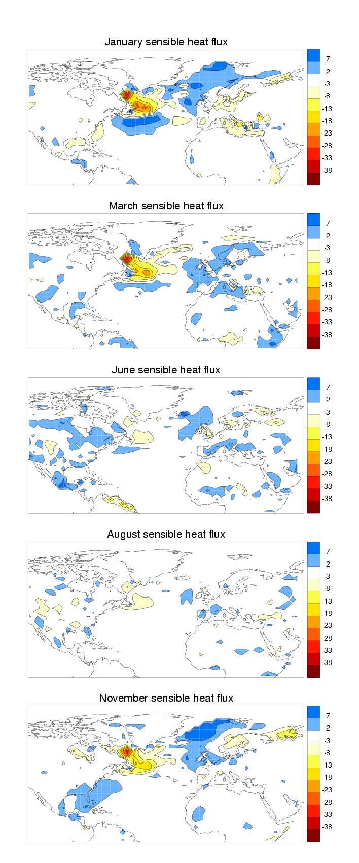
41 41

42 42 Illustration 12 The precipitation anomalies during the first two weeks of the month studied. The color levels show the increase or decrease of precipitation in mm/day. The black thick line shows the 95% significance level. The significance level is calculated by a paired students t-test. The paired restriction is an exception of this plot, other plots in this section do not have the paired restriction included in the calculation of significance.

43 This is particular true in the winter season. Furthermore, the air is more humid as a result of latent heat fluxes and therefore less evaporation will take place. Changes in windspeed and direction may also influence the magnitude of the heat fluxes. The impact on the atmosphere of the latent heat flux is where the warming energy is released. The areas with more condensation (latent energy release) and the areas with less condensation (lesser latent energy release) are shown by the precipitation anomalies. The precipitation anomalies during the first two weeks are shown in Illustration 12. In the first week of November, January and March positive precipitation anomalies are seen over the SST anomaly. During the second week the increase of precipitation over the SST anomaly is smaller than in the first week. In November and January is a tendency to an increase farther to the North. In section is the precipitation anomalies in the last two periods of the five months shown and therefore also the areas with the impact of the latent heat flux. 43 Illustration 13 The daily varying anomalous latent and sensible heat flux through each of the studied months. The heat flux is averaged over the area of the maximum of the SST anomaly. The model calculates the heat flux as positive from atmosphere to ocean. The SST anomaly is kept constant during the model run and does not

44 44 cool as a result of the heat fluxes, but the atmosphere is free to respond and adjust by temperature and humidity to the fluxes from the ocean. Theoretically this should lead to a reduction in the anomalous heat fluxes during time (Peng and Whitaker 1999), but this is not the case in the timespan of any of these experiments. Instead the average heat fluxes stay at the same level through out the runs (Illustration 13). A small increase in the variability of both the latent heat fluxes and the sensible heat fluxes occur near the end of the month (not shown) The temperature and vorticity response The air is warmed up in a shallow layer below 900 hpa over the SST anomaly in all five months. A deep warm anomaly into the atmosphere is only seen during the entire month in January. In the remaining months no stable deep temperature response occur. In the third week of June and November the warming anomalies have a pattern which may be compared with the pattern seen in the end of January (Illustration 14). The air temperature is increased from sea level and up to 300hPa, above this level the air temperature decreases, slightly downstream the pattern is reversed; the air is cooled below 300hPa and heated above this level. In the third week of June and November a third reversal of the pattern is seen with again a low level warming and upper level heating. This is connected to the wave train response seen in the geopotential height field, which is shown in Illustration 18 and described in subsection As discussed in the introduction an external Rossby wave is a barotropic wave train with maximum anomalies in the pressure field in the upper atmosphere and with warming anomalies below the high pressures and cooling below the low pressures (Held et al. 2002). Furthermore, the wave trains are seen to have a slight bending towards the Equator as they are following the first part of a great circle, and this is the typical path of a Rossby wave (Branstator 1983). Therefore, these three wave trains are considered to be stationary Rossby waves. The vorticity field follows the gradient of the temperature. Positive vorticity (i.e. low pressure) is added where the anomalous dt/dz is positive, and negative vorticity (i.e. high pressure) is added where dt/dz is negative (Illustration 15) (Kushnir et al. 2002). The temperature near the surface changes over large areas of the Northern Hemisphere but not in the same pattern through each month, and notable areas above the 95% confidence level are only found in January. The Arctic area north of the SST anomaly is warmed up in January. In particular an area in North West Canada and Alaska has a significant temperature anomaly above 2.5 K in the last period of the month. The middle and southern part of North America and Europe are cooled. This means that the anomalous warming of the North Atlantic results in a colder weather for most of the populated areas of the Northern Hemisphere in January. The cooling anomalies are below the 95% confidence level for the most part, despite a temperature decrease of for instance 2 K in Europe. The similarity between period 3 and period 4 suggests that this could be a real response. The result may also be compared with the results in chapter 4. In chapter 4 a North Atlantic SST anomaly pattern is connected to a cold Europe in winter, when the polarity of the SST anomaly pattern is negative (the pattern has a warm pole in the same location as the SST anomaly in the experiment of this chapter). The other months studied have temperature anomalies below the significance level almost everywhere, and the patterns of warming and cooling do not

45 resemble the other months. For instance the 2 m temperature changes of March are approximately antisymmetric to the anomaly pattern in January. August has generally smaller temperature anomalies than the other months 4. It is not surprising that the response patterns are changing through different months, since the different background flows in the months are suspected to highly influence the response patterns (Peng et al. 1995; Peng et al. 1997; Hall et al. 2002; Walter et al. 2002). The 2 meter temperature above the ocean is strongly connected to the ocean temperatures, which are prescribed in the model runs. Therefore larger temperature changes are almost impossible over the ocean, except directly above the SST anomaly or above sea ice (Illustration 16). 45 (the following three pages show three illustrations) Illustration 14 The anomalous heating above the SST anomaly. A slice is taken through the atmosphere at 52 N and the SST anomaly is placed approximately between S. Each full line and color level in the plot shows an increase of 0.5 K and each dotted line and color level a decrease of the same magnitude. The zero line is not drawn. Illustration 15 The vorticity changes above the SST anomaly. The slice through the atmosphere is taken at 52 N. The SST anomaly is between S. Each full line and color level in the plot shows an increase of 2*10 6 s -1 and each dotted line and color level a decrease of the same magnitude. The zeroline is not drawn. Illustration 16.The 2 meter temperature changes for the last two periods of the months. Each color level represent an increase or decrease of 0.5 K. The thick black lines show levels of significance. Above the SST anomaly the confidence level is above 99%. Elsewhere one thin black line show the 90% confidence level and the thick black line is the 95% confidence level. 4 Plots of 2 meter temperature for June does not exist, since I do not have these data from the model runs of this month.

46 46

47 47

48 48

49 2.2.3 The stormtrack response The stormtrack is calculated with the Poor Mans method. This method is used because of its simplicity. It does not need data points outside the time period of interest as a full frequency analysis with a bandpass filter (Palmer and Sun 1985). In this model setup the perturbed experiment is not run for more than the actual month in question making data points outside the month unavailable. When calculating the stormtrack by the Poor Mans method, the variance is found for each five day non overlapping period, and the variance is thereafter averaged over the 5 days periods. Few similarities between the stormtrack changes in the different months are found. In the winter cold and dry air is advected from land to the warm ocean, which is related to a strong baroclinicity. The anomalous temperature gradient is seen at 2 meter in Illustration 16. The baroclinicity is increased at the coast area and the stormtrack is intensified west of the SST anomaly in November and January. The baroclinicity is according to theory strongly connected to the release of latent heat (Chang et al. 2002). The release of latent heat in the two first weeks is shown in Illustration 12 and the release of latent heat in the remaining part of the month is shown in Illustration 21. It may be noted that particular during the first week an anomalous latent heat release takes place in the area of increased stormtrack activity in the winter months. During the summer the temperature differences are smaller and the air over the land is warmer than the air over the ocean, and in June and August there are only small changes in the stormtrack above the coast area west of the SST anomaly. Other weakenings and intensifications of the variability are occurring in different geographical areas, but with few similarities between the different months (Illustration 17) Local response in geopotential height In January a high pressure anomaly is created above the SST anomaly during the first two weeks and it moves slightly downstream during the rest of the month. The high pressure anomaly has a barotropic structure from the beginning to the end of the month (not shown, but may be indirectly seen in the vorticity anomaly plot, Illustration 15). If the initial response is baroclinic, as suggested in theory (Peng and Whitaker 1999, Kushnir et al. 2002), it does not show up in the timescales of the average response in this study. An average of the first three days of the geopotential height anomalies was taken in order to examine the existence of an initial baroclinic response (not shown). The weak response of this timescale is also barotropic. A wave train follows the high pressure anomaly. The high pressure anomaly is followed by a low pressure system over Europe and an additional high pressure system over the Arabian peninsula. The pattern of the pressure anomalies bends towards the Equator. The two anomalies over Europe and the Arabian Peninsula are above the 95% confidence level at 500 hpa at the end of the month. The first high pressure anomaly over the North Atlantic is above the 90% confidence level in the third week but loses significance by the end of the month. In June a smaller high pressure anomaly appears in the third week and is followed by a low pressure system above Europe much like the January response. In the third week the two systems are above the 95% confidence level, but in the last quarter of the month the high pressure anomaly moves upstream and the low pressure anomaly disappears (Illustration 18). 49

50 50 Illustration 17The stormtrack response of the last 10 days of the month. Each color level represents an increase of 25 m² of the 500 hpa geopotential height 1 to 5 days variance (5 m deviation). The zeroline is omitted. The black thick line indicate the 95% confidence level. The variance of the stormtrack is calculated by the Poor Mans method described in the text.

51 Illustration 18 a. The changes in the geopotential height at 500 hpa for November and January. Period 1-3 are the first 3 weeks of the month, period 4 is the remaining 10 days of the month. Each color represents an increase or a decrease of 10 m of the anomalous geopotential height as indicated by the color bars. The zero level between -10 m and 10 m is not shown. The black thick lines show the significance levels. The first line is where the anomaly is above the 90% confidence level, and the second show the 95% confidence level. 51

52 52 Illustration 18 b. The changes in the geopotential height at 500 hpa for March and June.

53 Illustration 18 c. The changes in the geopotential height at 500 hpa for August. 53

54 54 In the third week of November anomalies of high pressure, low pressure and high pressure are again distributed much as seen in January. However, only the latter high pressure in the subtropics is above the 95% confidence level. In the end of the month the high pressure has moved downstream and the wave train signature is broken up. All three described wave patterns appear to follow the path of a great circle. In the geopotential height plots from August and March no local distinguishable wave trains appear in the averages. Illustration 19 The square drawn in The North Atlantic of the world map shows the area where the geopotential height for the PDF-distributions is from. The five histograms for each of the five months show the PDF-distribution of the geopotential height at 500 hpa. The black histogram is for the control run and the red histogram is for the perturbed run. Each interval of the histograms is 50 meters Probability density function The atmospheric response in the local field is found in the average of the ensemble. The possibility exists that the average does not give a good representation of a change. The atmosphere could respond by increasing the probability of two different regimes. This is in line with the Lorenz attractor in which two attractors exist in a chaotic system (Ott 1993). If the atmospheric system changes by splitting one attractor in two, the average may not show it. Changes of this kind should be seen in the probability density function (PDF) of the atmospheric parameter. The PDF is calculated for the 500 hpa geopotential height slightly downstream from the

55 maximum SST anomaly. The geopotential height is found as an average over a small area. The values for each day in each of the ensemble members are systematized and plotted in a histogram with steps of 50 meters. The area chosen is where the geopotential field shows a high pressure anomaly in January, and it is in approximately this area most studies discuss the atmospheric response. The result does not show any significant change in the shape of the probability function between the control and the perturbed model run for any of the months studied. The five months have a seasonal variation of the shape and position of the PDF distribution. The shape of the PDF is higher and thinner in June and particularly August than in November, January and March. This is an indication of a smaller variability in the summer than during winter. In January the position of the PDF distribution shifts to larger geopotential height values from the control run to the perturbed run (Illustration 19) Upper tropospheric zonal wind and wave train crossing the Equator In January the wave train is seen to bend towards the Equator. The pattern is significant in the geopotential height anomalies at the 95% level at 500hPa (Illustration 18). At the Equator the control run with climatological SST shows an average westerly wind in January over the Pacific and in a small area over the Indian Ocean. This is of interest if energy via Rossby waves should cross the Equator. As discussed in the introduction the standing Rossby waves exists only on a westerly flow. It is seen that the January wave train may be followed in the upper troposphere across the Equator. 55 Illustration 20 The vorticity anomaly at 250 hpa in the last 9 days of January. Each color level represents an increase of 0.4*10 6. The black lines indicate anomalies above the 95% significance level. The vorticity plots of 250 hpa show an extension of the January wave train from the Arabian peninsula to India and over the Indian ocean in the last part of the month (Illustration 20). A crossing of the Equator by another apparent wave train is also seen in

56 56 the Pacific Ocean. This wave train may also be followed from the SST anomaly. The 2 meter temperature shows an anomalous warming over North West Canada and Alaska (Illustration 16). The warming is probably caused partly by advection of the anomalous heat from the SST anomaly and partly by anomalous winds and anomalous transient eddies, which also are a result of the SST anomaly. A high pressure anomaly in geopotential height appears above the temperatur anomaly in North West Canada in the third week of January together with a low pressure anomaly over the North Pacific (Illustration 18). The anomalies may also be seen in the 250 hpa vorticity field in the third week of January but with no clear wave train path to the Southern Hemisphere (not shown) Teleconnected effects in geopotential height Remote statistically significant responses are seen at different locations in the last period of all of the months (Illustration 18). In June, several geopotential height anomalies are seen all around the globe in the subtropics and midlatitudes of the Northern Hemisphere. The anomalies are distributed with intervals similar to a planetary wavenumber 6. A low pressure anomaly over Sibiria also appears. In August, November, January and March the anomalous geopotential height fields show a pattern with a low pressure system in the Indian ocean on the Southern Hemisphere. The pattern is similar in November and January. The low pressure anomaly is flanked by two high pressure anomalies to the east and the west. In March the pattern is found slightly displaced towards the west. In August the position of the low pressure anomaly lies more to the west than the other three months and there are not any connected high pressure systems. In both August and November a high pressure anomaly appears in the southern Pacific. The southern hemispheric pressure anomalies are all barotropic in structure (not shown). At both hemispheres the stormtracks are intensified during the winter months. The variability is larger and spontaneously occurring anomalies are therefore also larger. This may be seen in the plots as generally larger atmospheric anomalies in the Northern Hemisphere in January and November, and in the Southern Hemisphere the anomalies are generally larger in June and August. This should be taking into consideration when interpreting the results of the simulations. The geopotential height anomalies in the Indian ocean are largest and most significant in the fourth period of the months. In the third period the patterns are not present. The high pressure anomaly pattern in the southern Pacific is already present in the second period of August and in the third period of November. Several other patterns may be found in the different months. March, August and November are examples. In March, a high pressure pattern in the southern Pacific resembling the pattern in August and November is seen, but it is not above the significance level in March. Another pattern is found in November, June and partly January, these months have a tendency to a high pressure anomaly near the Aleutian low.

57 57 Illustration 21 The precipitation anomalies for the five months studied. The precipitation is given in mm pr. day and as an average for the last two periods of the month. The color levels are shown in the color bar. Blue indicates more precipitation and red less precipitation. The color indications start where the anomaly is more than 0.25 mm pr day and each increasing level is at 0.25 mm. The 95% confidence level is shown by the black thick line Precipitation The locally increased evaporation from the sea surface and the increased moisture in the air together with changes in temperature, wind directions and

58 58 stormtrack lead to changes in the precipitation. The release of heat from the latent heat flux is in the areas with increased precipitation. In section the latent and sensible heat flux was discussed. It was shown that the precipitation anomalies in the first week of the month are approximately over the SST-anomaly in November, January and March (Illustration 12). In the second week the precipitation anomalies get less significant and the increase in precipitation has a tendency to be advected slightly towards the north. The changes in precipitation in the last part of the month are shown in Illustration 21. The precipitation increase in the local area is placed slightly to the north of the SST anomaly in November, March and January. The air transported towards the north is warmer and more moist than usual, which increases precipitation when the air is cooled down and the moisture condenses. The precipitation anomalies are different during the summer months. June has an increase of precipitation north of the SST anomaly, but more northeast of the SST anomaly than seen in the winter months. August shows no local changes which exceeds the 95% confidence level, and the small changes are close to the opposite of what is seen in June (Illustration 21). 2.3 Discussion The areas of significance in the atmospheric response are few and small. Random sampled values should exceed the 90% significance level in 10% of the times the students t-test are calculated, and the 95% significance level should be exceeded in 5% of the times. Most fields in these experiments do not have a higher percentage of the area which exceed the significance levels. To find a significant result or to exclude areas which have shown a significant response several more members in each ensembles are needed. However, the number of members in the ensemble has been constrained by the time consume it takes to perform the runs and the computer time available. Furthermore, it is also judged that if 20 members are to few members in an ensemble to get a significant result, the signal to noise ratio is probably also too low to have any usable applications for seasonal predictions. The conclusions drawn from the results of this experiment should be and have been done under consideration of the low significance. The patterns of latent and sensible surface heat flux introduced by the SST anomaly have similarities in the local field in all of the five months studied. The size of the anomalies has a seasonal variation, but the pattern is the same. It is characterized by an increase of the energy flux to the atmosphere above the SST anomaly and a surrounding decrease. The different atmospheric responses are connected to the penetration of the heat fluxes into the atmosphere and the location of the associated latent heat release. The air over the SST anomaly is only warmed in a shallow layer below 900 hpa in all simulation, but in some simulations the anomalous temperature increase reaches farther up in the atmosphere. A wave train appears when the penetration of the temperature anomaly is up to 500hPa. The sensible heat flux is warming the air directly above the SST anomaly, but the latent heat flux is warming the air in the areas where the increased moisture condensates (i.e. increased precipitation), and may therefore have a more

59 remote impact. This impact can be seen in the precipitation anomalies. During the first week a significant precipitation anomaly is seen over the SST anomaly in November, March and January. During the following weeks the increase in precipitation are displaced slightly to the north of the SST anomaly and several other anomalies of increase and decrease appear. The changes in precipitation are mostly non-significant in the last part of the month. The local increase in precipitation north of the SST anomaly in the winter can be explained by the latent heat flux is released here. Therefore, confidence may be put in this result. The release of latent heat should increase the available potential energy for eddy generation (Chang et al. 2002) (see section 1.2.3). The changes in the intensity of the stormtrack are therefore expected to be close to or in connection with the areas where the anomalous latent heat is released. In the winter is seen a significant intensification of the stormtrack slightly west of the SST anomaly. As already mentioned; a increase of precipitation is seen in the first weeks in this area but during the rest of the month the pattern changes and areas of significance are small and few. The 2 meter temperature shows the ocean air is warmed and the middle of the North American continent in general is cooled during winter. This could indicate a increased baroclinicity which is related to the intensified stormtrack over New Foundland seen in the simulations. The pressure field's atmospheric response in the area surrounding the extratropical SST anomaly has a different size and pattern in the five different months. This is expected from the different background conditions, but the atmospheric responses are also different from week to week in each of the months. As an example the geopotential height field of November shows a high pressure over the SST anomaly followed by a low pressure over Western Europe in the third period, while in the fourth period the pattern is opposite with a low pressure directly above the SST anomaly and a high pressure over Europe (Illustration 18). Another example is seen in June, where a high pressure anomaly is present over the North Atlantic in period 3 with a downstream low pressure over Europe, but in period 4 the low pressure anomaly over Europe is changed to a high pressure anomaly. In August all responses seem to have disappeared in the averaging. The atmospheric response is dependent on the background flow. It is possible that the changes introduced by internal variations of the atmosphere can change the background flow to a degree to which they may dominate the nature of the response. In this case it is not possible in this area to use SST anomalies for forecasts other than the short timescale predictions for the weather. As soon as the chaotic variation of the atmosphere diminishes the predictability from the initial state, the predictability gained from SSTs also starts to disappear. Only if a 'preferred response pattern' which is less sensitive to the background flow exists, it may be possible to predict a response in this area. This 'preferred response pattern' may even be located in a remote area from the SST anomaly. A preferred high pressure anomaly over the North Atlantic in January may exist, but it is not significant in this study and none of the other months studied show a stable response in the local field. The atmospheric anomalies in the Indian ocean have a larger similarity 59

60 60 in pattern and a higher significance than the local effects of the SST anomaly. This is surprising. The energy introduced to the atmosphere in the North Atlantic has to cross the Equator, if the southern hemispheric response is a result of the SST anomaly. The crossing of the Equator could be by teleconnection of global long Rossby waves. However, if the energy transport to the Southern Hemisphere is by Rossby waves, the path of the wave trains are not the same during each experiment. If the paths were the same in each simulation this would result in a wave train pattern standing out in the average anomalies. In most plots this kind of wave train is not seen in the average. In some months are indications of a wave train starting over the SST anomaly and taking the path over Europe and south over the Arabian peninsula. This wave train is most significant in January and it is found to cross the Equator in the upper troposphere. The vorticity anomalies in the upper troposphere also show a wave train crossing the Equator in the Pacific. Likely several wave trains cross the Equator but are not visible in the average because of different patterns and paths in the different members of the ensemble. The significant anomalies on the Southern Hemisphere may be the result of preferred patterns in the southern hemispheric stormtrack, which have caused the different waves to align and adjust to the same wavelength and phase. It has been suggested that the northern hemispheric stormtracks have preferred areas where the response will appear, when a heating or cooling anomaly is introduced, and as mentioned in the chapter 1 simplified experiments have shown that while the linear response due to the direct thermal forcing will follow a displacement of the SST anomaly, the nonlinear eddy forced part of the response may stay in place. The present experiment indicates that the southern stormtrack has a preferred response pattern in the Indian ocean and also during some months in the southern Pacific. The connection to the real atmospheric responses to SST anomalies is questionable. It depends on whether a similarity exists between the models preferred southern hemispheric patterns and the real atmospheres preferred patterns, and if the teleconnection between the Northern Hemisphere and Southern Hemisphere is equally strong in the real atmosphere and the model. Off course, the possibility also exists, that the response are occurring by a statistical change. The results of this experiment have not been compared to observational data. It has been mentioned that the remote response's connection to the real atmosphere's preferred response patterns are considered questionable. Furthermore, the response patterns in this experiment are those to an idealized SST anomaly. Mathematical techniques as regression analysis of the SST anomaly on observed SST data fields and correlation of this result with observed data would be necessary in order to make comparison with the real atmosphere. It will not be possible to completely eliminate effects of other SST anomalies in other regions of the world and the observed data sets are also of a limited time period. The doubt that the response is similar with response patterns in the real world, the time consume connected to the analysis needed for this comparison and the believe that any possible connections are to small to appear in such an analysis have lead to the decision of not comparing the model results with observed data. 2.4 Conclusion The North Atlantic warm SST anomaly introduces energy to the atmosphere through the latent and sensible heat fluxes. An increase of heat flux above

61 the SST anomaly and a smaller decrease downstream in the eastern end of the North Atlantic ocean and south of the heating anomaly are seen. The latter does not apply for November. The latent heat flux anomalies lead to a local precipitation increase above the SST anomaly in the first week and later in the months to a precipitation increase north of the SST anomaly during winter. The North Atlantic stormtrack is intensified slightly west of the SST anomaly in January and November. The strength of the stormtrack is connected to the baroclinicity of the atmosphere and this may be related to the latent heat release, which is seen in the precipitation anomalies. The effect of the extratropical SST anomaly seems to be on a global scale. Statistical significant responses are seen around the Northern Hemisphere in June with a distribution as a planetary wavenumber 6. November and August have a high pressure anomaly in the South Pacific at the end of the month. January, March, August and November all have statistically significant responses in the Indian ocean, with an identical pattern in November and January. These results indicate an importance of 'preferred response patterns' for the atmospheric response of the model. In the local area the SST anomaly generates a wave train of high pressure and low pressure systems in January. The same pattern is seen in the third week of June and August. When the wave train pattern appears in the average geopotential height, it coincides with the heating anomaly penetrating up to the 500 hpa level in the atmosphere. The energy transport from the local area to the Southern Hemisphere is possible by wave trains starting in the local area and crossing the Equator. In January a wave train is found to cross the Equator over the Indian Ocean in the upper troposphere through a gap in the critical zones of easterly winds. The original motivation for studying the response to a warm North Atlantic SST anomaly was to find forecast possibilities for Europe in a monthly timescale. The response in all of the studied parameters shows almost no significance in Europe and no pattern similarities are found from month to month in the atmospheric response either. This study does not indicate any possibility for forecast from SST anomalies in this timescale for Europe. In the introduction of this experiment was presented the theory that the averaged response of a season could be misleading since the response may change during a season with changing climatologies in the different months (Peng et al. 1995; Peng et al. 1997). This study does not show responses of a larger magnitude than is seen in other experiments with averaged responses over different seasons (Palmer and Sun 1985; Ferranti et al. 1994; Lopez et al. 2000; Peng et al. 2002). A seasonal response to an idealized SST pattern will later be shown in chapter 4. It will be shown that the responses are of the same magnitude as the atmospheric anomalies in the experiment in this chapter. The simulations in this chapter show that the response in the local area are changing throughout the timespan of only one month. The remote response patterns are to some degree similar in different months (e.g. The Indian Ocean pattern in November and January and the South Pacific anomaly in August and November). This indicate that a seasonal average may lead to a higher significance of these patterns. Therefore, it is concluded that it is not misleading to average the atmospheric response over a season and that 'preferred response patterns' in the model are important for the atmospheric response and these preferred patterns can be the same through several months. If seasonal prediction is to be made it is important to determine the preferred response patterns of the real atmosphere. 61

62

63 3 A model experiment forced by observed SST anomalies The ocean has an effect on the variability of the atmosphere, but the magnitude of the influence may be different at different timescales. In the introduction is described how the low frequent variability of an AGCM is enhanced when an ocean model is coupled to the atmospheric model. It is also described how the frequency spectrum of the observational winter NAO is red with peaks at periods of decadal timescales (section chapter 1). These are both indications of an oceanic influence on multi-annual to decadal timescale. The theory was presented, that the ocean influences the extratropical atmosphere by adjusting to the atmospheric forcing and thereby provides a damping of the heat fluxes. This could cause a red spectrum of the atmospheric variability as seen in observations. But if the influence of the ocean is only a feedback to the atmospheric anomalies, predictability of more than a few seasons could be impossible. The question is: If an oceanic anomaly is known, but the state of the atmosphere is not known, is it then possible to make predictions about the variability of the extratropical atmosphere? A hypothetical example could be: An ocean anomaly is predicted to follow the North Atlantic Current through the next few years. Is it possible to predict the influence this anomaly will have on the NAO? The SST anomaly has to have a direct impact on the atmosphere which is large enough to be predicted. The following experiment is designed to test if a significant part of the low frequency variability is generated by direct SST forcing. The model is forced with prescribed SSTs and the ocean cannot adjust to the atmosphere. The AGCM used is the ECHAM4 model. (see appendix 7.3). The potential predictability (PP) of the atmospheric variability for different geographical areas in four seasons is found. The North Atlantic and the European area is of particular interest. The NAO of the model is also analyzed. In the following chapter and the rest of the thesis an abbreviation is used for the seasons (December, January, February (DJF), March, April, May (MAM), June, July, August (JJA), September, October, November (SON)) and an abbreviation for potential predictability (PP) The PREDICATE project A part of the data analysis described in this chapter is used in the PREDICATE project. It is to be published in a paper with Laurent Terray as main author (Terray et al. 2003). PREDICATE (Predictability of Decadal Fluctuations in Atlantic-European Climate) is a European project under the fifth framework program of the European Commission. It belongs to Key Action2: "Global Change, Climate and Biodiversity" within the Energy, Environment and Sustainable Development thematic programme, with contract number: EVK2-CT Scientists from England (UGAMP, The Met. Office), Germany (MPI), France (LODYC, CERFACS), Norway (NRSC), Italy (ING) and Denmark (DMI) have participated in the project. 63

64 64 The project investigates climate variability and predictability in a 2 to 20 years timescale. Model experiments of the AMIP type, experiments with coupled models and experiments with idealized SST anomalies are included in the project. 3.1 The setup of the experiment The data used in this experiment were provided by the Max-Planck- Institute für Meteorologie in Hamburg, where the ECHAM models were developed. The model runs are of the AMIP type (atmospheric model forced with observed SST and sea ice). A description of the model (ECHAM4 in a T42L19 setup) is in appendix 7.3. SST variations and sea-ice coverages from the GIST2.2 data series are used as the boundary forcing. The GISST2.2 includes monthly mean SST and sea-ice coverage from , and they are available from The British Atmospheric Data Center (BADC : The SST and ice cover variations are observations interpolated into global coverages and a regular grid. EOF reconstructing is used for the creation of the dataset. The GISST data are a combination between the Met Office Historical Sea Surface Temperatures (MOHSST6) of the British Atmospheric Data Center and the Walsh Sea Ice Concentration data from National Center of Atmospheric Research (NCAR). The MOHSST6 data start in 1856 and the Walsh Sea Ice Concentration Dataset starts in 1870 (Rayner et al. 1996, Walsh and Chapman guide to the data set, BADC). The confidence in the data set is of changing degree through the years. The Walsh Sea Ice Concentration Dataset undergoes a great improvement in 1951, from this time and forward almost complete northern hemispheric observational coverage is obtained. Prior to this time several areas with missing data were filled with climatological values. The southern hemispheric data must still be regarded with caution after 1951, particular areas south of 45 S where only sparse data exist. (Rayner et al. 1996, Walsh and Chapman guide to the data set, BADC) Six different ECHAM4 model runs forced by the GISST2.2 data set were available. Four of the runs are initiated with the GIST2.2 data from 1903 and continue until 1994, and two of the runs are initiated with data from 1951 and continue until Weaknesses of the experimental design The simulation is a hindcast run, where the full variability of the SST anomalies is prescribed. This is not possible in a forecast experiment. Furthermore the AGCM is assumed 'perfect' in the analyse of the PP (potential predictability). It is the models ability to predict its own low frequency variability and not the ability to predict the variability in the real atmosphere which is investigated. Because of the full variability of the SSTs and the assumption of the model is perfect, it may be seen as an upper bound of the predictability which can be achieved with the model. The analysis is therefore called potential predictability. However, problems also exist with the interpretation of the results as an upper bound. The AGCM may have errors and the effect of SST anomalies may be underestimated or misrepresented in the model. Furthermore, the model design does

65 not allow the ocean to adjust to the atmosphere. An adjustment between ocean and atmosphere dampens the heat fluxes and increases the low frequency variability of the atmosphere, and this is only partly possible in the setup since only the atmosphere may adjust. It may be impossible for the atmosphere to adjust completely to the ocean forcing. The modes of the model atmosphere are not exactly as the modes seen in observations (The modes of the atmosphere could be the EOFs or the stormtrack position which somewhat differ from the real atmosphere). The modes of the observational SST are exactly as known from the real ocean and atmosphere interactions, but the modes of the model atmosphere are slightly different. Therefore, erroneous heat fluxes may be created, since the modes of the AGCM atmosphere and the SST do not fit with each other completely. 3.2 The potential predictability (PP) calculation The mathematical method used for the variability analysis and PP calculations is from the paper by Rowell and Zwiers (1999). They provide a method where analysis of variance (often called ANOVA) may be calculated at different frequency ranges of the spectrum and the significance of the result may also be calculated. The method is described in details in appendix. A short description of the method is given here: The variance of the ensemble mean can be seen as the first guess of the variance caused by SST. However, due to a limited number of ensemble members the variance is contaminated by 'noise' from the internal variance of the atmosphere. The internal variance is estimated from the variance between individual members of the ensemble. The first guess on the SST induced variance is then improved by subtracting an estimation of the effect of internal variance. The PP is then given by the new estimated value of the SST induced variability divided by the full variability. The equation for the PP may be rewritten in terms dependent on an F- distribution. This is a distribution which can be found in a table of mathematical distributions. From the significance levels of the F-distribution the significance levels of the PP is calculated. The method of calculating the PP can be divided into different frequency ranges. The equations for the PP include time series where the variance is calculated. Data time series may be transformed to frequency space by Fourier transform. In frequency space a certain frequency range can be chosen and the rest of the data disregarded. This will effect the significance level of the result, but Rowell and Zwiers method to calculate the significance includes a dependency on how many 'frequency points' there are used in the PP calculation. The PP need to be higher to reach the 95% confidence level when a smaller frequency band is used. Illustration shows the number of 'frequency points' or the length of the smallest period included in the analysis and its connection to the PP value for 95% significance. The calculation of PP can turn out to be negative, and negative results are seen in the plots shown of the zonal PP. The negative PP is physical impossible, but may happen in the calculation if the estimate of internal variance is larger than the first estimate of SST caused variance. 65

66 66 Methods exist which should improve the signal to noise ratio in the calculations of the SST forced signals. For instance, in Yang et al. (1998) is a method described and another in Venzke et al. (1999). EOF analysis is used in both models to extract the modes of the atmospheric variability with a high signal to noise ratio. However, it is important to remember, that the chance of finding erroneous signals is higher the more alteration of data and the more sophisticated methods there are used. The methods may be very good at finding a signal contaminated in noise, but if the signal is not at all visible in the original data it must be considered if it is a pure mathematical constructed mode. Illustration 22 The minimum potential predictability needed to exceed the 95% confidence level. The upper plot shows the dependency of the number of 'frequency points' in the calculation. The bottom plot shows the minimum potential predictability as a function of the minimum year-period included in the calculation. As an examble: If only periods longer than 6 years are included, the minimum potential predictability necessary for 95% confidence is approximately 12%. 3.3 Results The SST forced variability at different frequencies In the following the frequency distribution of the variance caused by SST in the time range from 2 to 40 years is shown. In the PP analysis the relative variance is calculated (SST induced variance divided by full variance), this is a little different from the plots shown in this section. I have chosen to show the variance directly induced by SST, since most peaks are more distinctive here. The SST induced variance in the tropical Pacific has distinctive peaks at 3.5 and 5 years, this is the approximate timescale of the recurrent El Niño events. An average of the SST induced variability in a belt around the Equator shows the peaks even more clearly. The peaks of 3.5 years and 5 years are also seen in the

67 midlatitudes. The peaks are most distinct in the DJF season both in the Tropics and in the midlatitudes, and also in the North Atlantic - European area alone. (Illustration 23) 67 Illustration 23 The SST induced variability of the atmosphere as function of frequency in different geographical areas. The geographical areas are shown in the map in the upper left corner. The y-axis of the line-plots shows an index value rather than an absolute value since the magnitude of variance is different in the Tropics and the midlatitudes. The peaks at 3.5 and 5 years are shown to be global.

68 68 A 'cut' frequency can be set to divide the 'low frequency' part from the 'high frequency' part of the spectrum. The cut frequency is chosen to be at 6.3 years. This frequency will put the El Niño peaks in the high frequency part and exclude them from the low frequency part. The exact period of 6.3 year is chosen because this fit with a whole number of frequency 'points' in the data. The low frequency part which include all periods longer than 6.3 years (in the 44 year long dataset) is called the 'low frequency part' or the 'decadal' timescale in this experiment. The frequency range between 2 years to 6.3 years is called the 'high frequency' part Zonal average of PP in the pressure fields The general distribution of the PP is in zonal bands, and the distribution of zonal mean PP has a bell shape. The highest predictability is in the Tropics, a steep decrease takes place in the subtropics and a somewhat flattening of the PP is seen in the midlatitudes and polar regions. In the Tropics the predictability is higher at 500hPa than at the surface and the seasonal variation is smaller. In the extratropics these differences are not seen. In general the PP for MSLP and at 500hPa is the same (Illustration 24). Illustration 24 The zonal mean of potential predictability. Negative latitudes are in Southern Hemisphere, positive latitudes are at Northern Hemisphere. The 95% confidence level is indicated by the dotted line The Tropics The tropical PP at decadal timescales is in general higher than the PP at high frequencies. Almost 85% of the atmospheric variation at 500hPa is determined by the SST in the decadal time range. The PP is slightly smaller for the MSLP and the MAM season has the lowest PP at both the high frequency part and the low frequencies part. The PP for DJF is highest in the high frequency part for MSLP. This is an exception from the general rule. In the boreal winter season (DJF) the persistence of El Niño is highest (Torrence and Webster 1998), and it is probably the predictability gained by El Niño that gives the high frequency part of the DJF season

69 69 higher PP than the low frequencies (Illustration 38). Illustration 25 The zonal mean of the potential predictability of MSLP and geopotential height at 500hPa. The low frequency part includes frequencies with periods longer than 6 years and the high frequency part includes frequencies with periods between 2 to 6 years. The 95% confidence level is indicated with a dotted line. The difference between low frequencies and high frequencies potential predictability is shown in the two last plots. At most latitudes the PP increases at decadal timescales.

70 The extratropics In the midlatitudes of the Northern Hemisphere the zonal average of PP is below 22%. The maximum PP is in the JJA season in the low frequency part of the spectrum. JJA, SON and MAM all have increased predictability in the low frequency part, but the northern winter season has increased predictability in the high frequency part of the spectrum. In DJF the PP is 15% at 50 N in the high frequency part of the spectrum and at low frequencies the PP is closer to 12% and falling more rapidly with increasing latitude. In the Southern Hemisphere the PP also increases at decadal timescales (Illustration 38). The bell shape of the zonal predictability has a tendency to be shifted towards the north in the JJA season and towards the south in DJF season. The PP follows the climate zones and the higher predictability is connected to higher temperatures and may therefore be seen to follow the summer season on each hemisphere to some degree The spatial distribution of PP for the pressure fields The Tropics The PP at sea level are more detailed than PP in the mid-troposphere. For MSLP the variability induced by SST is seen to be higher over the oceans than over the continents. The same division of the PP is seen in a much lesser degree at 500 hpa. The higher dependency of geographical location for MSLP is interpreted as a higher atmospheric connection to the local SST anomalies (Illustration 26 and 27). In the Pacific El Niño (and La Niña) region seasonal development can be followed in the PP. In MAM the PP is lowest, and the area with the highest predictability is the NINO 1+2 region (the NINO regions geographical extent is shown in appendix 7.3). The NINO1+2 region is the area closest to the South American coast where El Niño temperatures are first seen. The NINO4 region has low PP, particular at the southern side of Equator. The JJA, SON and DJF show a high PP above all the NINO-regions. In DJF a tongue of PP reaches towards the north off the North American coast. The PP is above 40% up to Alaska in the average over all frequencies (not shown). The largest part of this PP is from the high frequency region. In the plot of the high frequency part the PP is above 50% near the Aleutian low. The periods under 6 years include most of El Niño variability and this PP in the North Pacific is probably connected to the tropical phenomena (Illustration 26 and 27). A local tropical minimum of PP is seen in the Indian Ocean, the PP is though still as high as 70% in the area. The Indian Ocean temperatures may be used for prediction of the monsoon onset and rainfall (Clark et al. 2000). It is interesting to note that the SST in the tropical Indian ocean in the SON and DJF correlates with precipitation amounts over India the next JJA, but the correlations between SST and precipitation during the monsoon are smaller and non-significant (Clark et al. 2000). That is, the SST can be used for predictions of the rainfall more than half a year later, but the SST actually present during the monsoon season gives no estimate of the

71 rainfall. Illustration 26 The globally distribution of PP for MSLP. The upper four plots show the decadal PP in four seasons, and the lower four plots show the PP in the timescale of 2 to 6 years. PP is given in % of full variability. The white areas are below the 95% confidence level. 71

72 72 Illustration 27 The potential predictability for geopotential height at 500hPa. The upper four plots show the decadal PP in four seasons, and the lower four plots show the PP in the timescale of 2 to 6 years. PP is given in %. The white areas are below the 95% confidence level.

73 3.3.4 The North Atlantic European region The decadal timescales have a larger PP than the high frequency variations in most seasons and areas, and the decadal timescales have the largest PP in the JJA season followed by the SON season. The DJF season which includes effects of El Niño does not have a higher PP than the other seasons (Illustration 28 and 29). For MSLP the PP is in general highest above the ocean. A tongue of predictability from the south towards the north in the Atlantic ocean is seen in JJA in the low frequency part. The PP of the atmospheric variance reaches 30% in an area up to 60 N. The European land areas have very little potential predictability in all seasons and in all timescales. The PP is of the same magnitude both at the surface and at the 500hPa level. This is also seen in the rest of the extratropics of the Northern Hemispheres and at the extratropics of the Southern Hemisphere as well Zonal PP of 2 meter temperature The atmospheric 2 meter temperature follows the SST above the oceans, but it is the predictability of the temperature above the continents that is of interest. Therefore is the zonal mean of PP taken only at 'grid points' above land areas. The PP should be regarded with caution in the zonal bands with very few points over land The Tropics At the Equator the PP of the temperature is from 54% to 65% depending on the season. The SON season has the lowest predictability and JJA and MAM have the highest. The low PP for SON is particular seen in the high frequency part of the variance. Apparently the low predictability of the ENSO in the MSLP in MAM does not affect the predictability of the 2 meter temperature. In general the PP of the decadal changes has a higher predictability than the variance in the high frequency part, as it also was seen in the PP of pressure. The DJF season is the exception, the PP is basically the same in the high frequencies and in the low frequencies. (Illustration 30) The extratropics Latitudes south of 45 S are of low confidence in the calculation of PP. Few land areas exist this far south with the exception of Antarctica, and the data used to force the model in this area are of low confidence. Therefore, the high zonal mean PP occurring at 50 S in the low frequencies is considered unimportant. 73

74 74 Illustration 28 The potential predictability of MSLP in the North Atlantic - European region.

75 Illustration 29 The potential predictability of geopotential height at 500hPa in the North Atlantic - European region. 75

76 76 In the Northern Hemisphere the PP in the midlatitudes is between 7% to 17% when all timescales are included (not shown). The potentially predictable part of the variance is low but statistically significant. As in the Tropics, a general increase in PP at the decadal timescales is found but the zonal mean PP does not exceed 20% in the area between 45 N to 65 N. The zonal mean PP north of 65 N is higher than in the midlatitudes at all frequencies, but the land areas here are almost only coastal regions and it is a relatively small area. The coastal areas are close to the known sea surface temperatures and the few data points at this latitude give less confidence to the result. (Illustration 30) Illustration 30 The PP of the 2 meter temperature as zonal mean over land areas The spatial distribution of PP for 2 meter temperature The PP of the 2 meter temperature above the ocean is between 80% to 100% almost everywhere. The PP is high because the temperature of the lowest atmospheric layer is heated or cooled by the temperature directly below, and this temperature is assumed known. The lack of data in the Southern Hemisphere south of 45 is seen in the spatial plots. Below 45 S the SST and ice data series become close to constant since the data are mostly climatological values. There is no variability in the forcing and therefore no atmospheric variability caused by the boundary conditions, which leads to zero PP The Tropics The highest tropical predictability is in the north-west of South America and the western part of the tropical Africa. The preference in the PP for the western parts of the continents may be caused by westerly winds which transport the ocean climate to the land areas, though other effects such as orography are also connected to the spatial distribution of the PP. (Illustration 34) The extratropics The European region has low PP. In most seasons and timescales the percentage of the PP is below 20%. The exception is the decadal PP in the SON season, in this season a part of mid-europe has a predictability above 30% and in JJA

77 77 another geographical area in mid-europe has PP above 20%. Illustration 31 The globally distribution of potential predictability of 2 meter temperature. The white areas in the plots are below the 95% confidence level. PP is given in %.

78 78 In North America the PP is highest in the winter and spring season. In the high frequency part of the variance the middle of Canada has a predictability from 30% and up to 50% in DJF. The same area has a PP above 30% in MAM. At decadal timescales the North American PP in JJA and SON is increased but it remains at approximately the same level in the DJF and MAM season Zonal PP of total precipitation The PP of precipitation is smaller than for other studied parameters. It exceeds 50% only in a narrow band of the Tropics during the JJA season. During almost all seasons the decadal variability has a higher predictability than the high frequency variability. In the Tropics, the JJA season has the highest predictability and in the northern extratropics the DJF season has the highest predictability. This is the case for both the decadal variability and the high frequency variability. In the polar region in the Northern Hemisphere, PP is high in all seasons except summer. In the low frequencies the zonal mean of the PP in DJF exceeds 30% in a small zonal band. Illustration 32 The zonal mean of potential predictability of precipitation. The dotted line indicate the 95% confidence level The spatial distribution of PP of precipitation Certain regions in the Tropics have a higher PP in the high than the low frequencies. Areas with a high PP in the 2 to 6 years range exist particularly in the El Niño region in the tropical Pacific. This is assumed to be connected to the periods of El Niño, which in the model is approximately 3.5 years and 5 years. The PP of the other ocean basins is smaller at high frequency than at low frequencies. A local minimum of PP is seen in the Indian Ocean at both low and high frequencies, the same area had a minimum in the PP of the pressure field (Illustration 32). In general the PP is higher over the oceans than over the land. The DJF decadal variations of precipitation in the North Pacific are between 20% to 40% in the low frequency part. In the North Atlantic some areas have the same magnitude of predictability as seen in the North Pacific, but over the European continent the PP is small and mostly unsignificant.

79 Illustration 33 The globally distribution of potential predictability of total precipitation. In the white areas the PP is below the 95% confidence level. PP is given in %. 79

80 80 In the Barents sea high percentages of PP are found. In the low frequencies in the DJF season PP exceeds values of 80% in the Barents sea. Such high PP values are in general not seen in the extratropics. The high PP values may be explained by a strong relation between the ice edge and the geographical area of precipitation. A seasonal variation of the position of the PP values is seen to follow the ice edge (Illustration 32). The position of the ice edge is prescribed in the experiment, and therefore the part of the precipitation connected to the shift from 'warm' ocean water to a cold sea ice cover is known. The result is a high PP in precipitation. However, in real forecasts the ice edge position are not known in advance Zonal PP of 10 meter wind squared In the calculation the square of the wind is used instead of the absolute value, since the kinetic energy of the wind is proportional to the square of the wind. The PP exceeds 50% in a narrow band in the Tropics, in the extratropics the PP is below 20%. At the Equator the JJA season has the highest predictability in both low and high frequencies. The maximum of zonal PP in the high frequency part is close to 52% and in the low frequency part the maximum is close to 58%. In general there is a slight increase in PP on decadal timescales. In the extratropics the season with the highest PP is DJF, but PP for most areas and seasons is below the significance level (Illustration 22). Illustration 34 The zonal mean of potential predictability of squared 10 meter wind. The dotted line shows the 95% confidence level The spatial distribution of PP of 10 meter square wind In the tropical Atlantic the plots show that the PP is highest at decadal timescales, in the Indian ocean the PP is also highest at decadal timescales but the differences between high and low frequencies are smaller. In the tropical Pacific the PP is almost equal at high and low frequencies. In the northern winter season an area near 40 N in the Pacific has PP close to 40% both at high and low frequencies. In the North Atlantic the PP is smaller.

81 Illustration 35 The globally distribution of potential predictability of squared 10 meter wind. In the white areas the PP are below the 95% confidence level. PP is given in % The NAO in ECHAM4 The NAO is closely linked to the North Atlantic and European climate. The NAO may be observed in the temporal evolution of the first EOF in the North Atlantic or in a more simple way as the difference between sea surface pressure at

82 82 Iceland and the Azores. In observations the two poles of the first EOF are close to Iceland and the Azores, hence the index of the temporal evolution of the EOF is almost the same as an index of the difference in pressure between the two measurement points. In a model simulation the simple method has the weakness that if the model does not have the two poles of the NAO placed close to the two measurement points the index loses meaning. However, the first EOF of the ECHAM4 model is similar to the EOF from observations, and the NAO is a large scale phenomenon where small deviations in geographic position are of little importance. In the following analysis it is shown that the anti-correlation between the two poles of the NAO is simulated well in the models, which indicates that the two poles of the NAO in the model may be found near Iceland and the Azores. The NAO is strongest in the winter season and weakest during the summer season (Illustration 36). The index is calculated as the difference in MSLP between the Azores and Iceland, thereafter the average is subtracted from the result. The data have not been normalized or further altered in any other way Correlation analysis Spearmans rank correlation is used instead of linear correlation in the correlation analysis. A rank correlation or a nonparametric correlation has the benefit compared to linear correlation that it is easy to find the significance of the correlation coefficient, even when the data are not from a two-dimensional Gaussian distribution (Press et al. 1994). When 'ranking' the data a small amount of information is lost and the Spearman correlation gives slightly different results compared to linear correlation, but it does not alter the conclusion drawn from the results. An example of the difference in the correlation by the linear method and by Spearman rank is seen in the correlation between the simulated NAO in the model and the NAO from observations. In the MAM season the linear correlation is and the Spearman rank correlation is (see table 1). The negative correlation between the two poles of the NAO is reproduced in the model with significant correlation coefficients in three seasons. The negative correlation between the MSLP at Iceland and the Azores exists in neither observations nor model simulations during the summer season. 5 Larger differences between linear correlation and Spearmans rank may be seen if other data series are chosen. For instance in the DJF season the linear correlation between the two poles of the NAO taken from observational data gives an correlation coefficient. The Spearman rank correlation gives a (significant) correlation coefficient at -0.74

83 Illustration 36 The NAO from the model simulations and observational data. Each of the 6 model runs is shown and the dotted line is the ensemble mean. The NAO from observational data is the thick black line. A significant correlation between the ensemble mean and the observational NAO is found in the MAM season. 83

84 84 DJF MAM JJA SON obs Az/Ic ens5 obs Az/Ic ens5 obs Az/Ic ens5 obs Az/Ic ens5 mod mod mod mod mod mod ens * * * * obs * * * * Table 1 The table shows correlations between the NAO from observations and the NAO from each individual member of the model runs. The correlation between the NAO from observations and the ensemble mean of the 6 model runs are also shown. In the second column of the table is shown the correlation between the two poles of the NAO at Iceland and the Azores. The third column shows each individual model runs correlation with the mean of the other 5 runs. This gives an estimate of the reproducibility of the NAO in the model. Correlations coefficients above the 95% confidence level is marked with red. In the spring, a significant correlation between the ensemble mean NAO and the NAO from observations is found. The individual members of the ensemble do not have a significant correlation with the observational NAO nor a significant correlation with the other members in the ensemble, with the exception of the first model run. The correlation between the ensemble mean and the NAO from observations is not significant in any other season Power spectrum of the NAO The power spectrum of the NAO is calculated from 1951 to 1994 for both the observed data and data of the model runs. The method used to calculate the spectrum is a segment overlapping method with a Bartlett window. The Bartlett window takes nearby frequencies into account and put less weight on frequencies farther away. The segment method should decrease peaks occurring by errors due to the numerical method and it should smooth the diagram of the power spectrum 6 (Press et al. 1994). The average power of all frequencies is similar for the observed data and for the individual members of the model runs. The spectrum of the ensemble mean of the model simulations has a smaller average power. This is due to a loss of variability in all frequencies when the ensemble mean is calculated. However, the periods of similar length in the different members of the ensemble remain in the spectrum of the ensemble mean. The change in atmospheric variability between seasons is also seen in the power spectrum. In the winter season the average power is approximately 10 times the power in the summer season. 6. The particular method used is the one described at page in Numerical Recipes. Three segments is used.

85 85 Illustration 37 The power spectral diagram of the NAO for both observational data and the model simulations. Note the different scales of the y-axis in the four seasons. The NAO is usually defined for the winter season, since it is strongest in this season. The power spectrum of the observed NAO is red in the winter. The model runs do not show a red spectrum consistent with the one seen from observations but show instead a more white signal. This may be caused by the lack of an interacting ocean. The ocean increases the low frequency variability by acting as a capacitor as described in the introduction, but this is not possible in an AMIP-type experiment. The power spectrum of the NAO is only red in the winter. In the other seasons the power spectrum of the ensemble mean has some similarities with the power spectrum of observed data, particular for the MAM season. In the spring season both the ensemble mean and the power spectrum of the observed NAO have a

86 86 distinct peak at 3.5 years (Illustration 37). This peaks coincide with one of the peaks induced by El Niño. In section was shown that the SSTs of El Niño resulted in two peaks in the variability spectrum of the North Atlantic caused by SST. The two peaks are at 3.5 years and 5 years El Niño signal in the NAO El Niño has a too strong correlation with the NAO of the ECHAM4 compared to the teleconnection in observations (see appendix 7.3). Therefore, it would be of interest to calculate the correlation coefficients between the model NAO and the observational NAO, when the effect of the El Niño is removed from the data. In the following the linear effect of El Niño is removed by linear regression from the data. The NAO of the ECHAM4 model has been correlated with different El Niño indices. The result is shown in appendix 7.3. The NINO3 SST index has a correlation coefficient at 0.30 with the NAO of the model in the MAM season and the NINO4 SST index has a correlation of The southern oscillation index (SOI) was also correlated with the NAO of the model. The SOI is an atmospheric index and it is taken from observations, therefore it must be assumed to fit better with the observed atmosphere than the model simulated atmosphere. Still the correlation with the NAO was high and significant in the model but not in the observations. The NINO4 index is considered to be the 'best' index for the removal of El Niño from the NAO by linear regression. The reason is that: The NINO4 index is an SST-index and therefore the same in the model and in the observational data and it has a better correlation with the NAO of the model than the NINO3 index. In the following correlation all three El Niño indices are used, so the results may be compared. The results show as expected that the NINO4 index is the best suited. A linear correlation with the particular El Niño index is calculated for both the model NAO and the observed NAO. The two resulting linear relations are then removed from the two NAO data series. The correlation coefficients are calculated between the new data series and shown in the table 2. The removal of El Niño from the data series does not weaken the correlation between the spring NAO in the model and in the observations. The correlation coefficient is actually increased when the NINO4 index is used for the linear regression. This indicates that it is other SST anomalies which are responsible for the 'good' simulation of the NAO in the model. The removal of the linear effect of El Niño does not improve the non-significant correlations in the other months. DJF MAM JJA SON Corr ens6 and obs SOI NINO NINO Table 2 The columns show the results from each season. The first row shows the 'old' correlation

87 between the ensemble mean from the model and the observed NAO, which includes the linear effect of El Niño. The three next rows are the correlation coefficient for the new data series, which have been subtracted the linear relation with the particular El Niño index. The correlation coefficients are calculated by Spearman rank and the results above the 95% confidence level are colored red in the table. El Niño is suspected to have an influence on the power spectral diagram peak at 3.5 years for the MAM model runs. A new power spectrum is calculated with the new data series. The data series chosen is those with El Niño removed by linear regression by NINO4 (Illustration 38). 87 Illustration 38 The power spectral diagram for the spring NAO in observations and the ensemble mean of the model simulations. The black lines represent the full data series and the red lines is after the removal of El Niño by linear regression with NINO4. The 3.5 years peak is basically unaltered in the observational data. This is not surprising since the connection between the NAO and El Niño is small in observations. In the NAO of the model a notable part of the 3.5 years peak is removed when the linear El Niño relationship is subtracted from the data. But the peak is still visible. It was examined if a better removal of El Niño could be done, if both the NINO4 and the NINO3 linear connection was removed from the NAO of the model. It did not further reduce the 3.5 years peak in the power spectral diagram (not shown). The linear correlation between the NAO and the NINO3 is close to zero when the linear correlation with the NINO4 is already subtracted from the data Predictive skill in the North Atlantic-European region The predictive skill of the ECHAM4 model is estimated from correlations between observed data and the ensemble mean of the model simulations.

88 88 The MSLP field and 2 meter temperature (T2m) from the ERA15 data series are used for the analysis (Gibson et. al. 1997). It should be noted that the T2m is model generated in the ERA data. T2m is highly dependent on cloud cover and soil moisture, which are two parameters not particular well simulated in models. Therefore the 'observed' data of T2m must be regarded with some caution MSLP The model simulation of MSLP is significantly correlated with observed data for large areas over the North Atlantic Ocean. The correlation coefficient is above 50% indicating that more than half of the variability in the pressure field may be predicted from the SST anomalies. High correlation coefficients are also found above Western Europe. Illustration 39 The correlation between the model's ensemble mean of 2 meter temperature and 2 meter temperature from ERA15-data (Gibson et. al. 1997). The correlation is calculated by Spearmans Rank. Correlations above approximately 0.50 are above the 95% significance level and areas of significance are indicated by a white contour. The high value of the correlation coefficient, which is needed for significance, is connected to the short data series. The ERA15 data-series is of only 15 years. In the spring season an area of high negative correlation is seen above the middle of Western Europe and Eastern North Atlantic. The negative correlation values are an indication that the model NAO is shifted relatively to the observed NAO. The NAO variability is close to observations, as it was shown in section , but apparently the dividing line between the Icelandic low and Azores high are different from the real world. The shift of the dividing line is also an indication of a shift in the position of the stormtrack. The high negative correlations are not seen in any other season or in any other geographical area. The lack of negative correlations

89 in the middle of the North Atlantic and the high positive correlations in the winter season are an indication that the NAO and stormtrack positions are closer to observations in the winter than in the spring. In the SON season a significant correlation between the model simulated MSLP and observations is found over Eastern Europe The 2 meter temperature The European temperatures are connected to the position of the stormtrack, but the shift of the stormtrack position in MAM is not large enough to alter the temperature to a degree of anti-correlation or low correlation. The correlation coefficient is above 0.30 for large parts of Europe in both the DJF season and the MAM season. The JJA season and the SON season have much smaller correlation values and JJA in particular has negative correlations in most of Europe. 89 Illustration 40 The correlation between the model's ensemble mean of 2 meter temperature and the 2 meter temperature from ERA15-data (Gibson et. al. 1997). Correlations above approximately 0.50 are above the 95% significance level, and areas of significance are indicated by a white contour. All correlations values above oceans are set to 0. The high correlations values of temperature in the MAM season may be expected from the model's predictive skill of the NAO, but the high correlation for T2m in DJF does not coincide with a high predictive skill of the NAO. 3.4 Discussion The pressure field has the highest PP of the atmospheric parameters studied and the precipitation and the mean square 10 meter wind have the lowest predictability. In general the PP is higher at the decadal timescales than in the frequency range between 2 and 6 years. The increase is caused by a higher variance explained by the SST at decadal timescales or/and a lesser variance explained by the

90 90 internal variability. The PP is high in the Tropics in all parameters studied. The zonal band with the high predictability is widest in the pressure fields (MSLP and 500hPa geopotential height). The temperature, precipitation and zonal wind anomalies have a smaller tropical zonal band with high predictability before the extratropical drop occurs. The seasons with the highest PP in the Tropics and the northern midlatitudes are shown in table 3. The table shows that in general the JJA season has the highest PP in the Tropics. Particular, the decadal variability is largest for the tropical JJA for all studied parameters. The high frequencies also have a maximum in the JJA season with the exception of the MSLP, which has a maximum in DJF. El Niño is strongest in the boreal winter season which probably explains the high PP in the high frequency part in the DJF season. In the northern midlatitudes the maximum in PP for the high frequencies is in the DJF season. The reason may be a strong influence of El Niño in this season. The teleconnection of El Niño is too strong in the model. Therefore, the relative high PP in the extratropics in DJF may be an erroneous model generated signal, if it is caused by El Niño. In the midlatitudes the maximum PP for the low frequencies is in the summer season for the pressure fields. For wind and temperature maximum PP is found during fall and winter, and maximum PP for precipitation is found during the winter. In all seasons and frequency ranges the spring season has a lower predictability. This is interesting when it is considered that this is the season where a significant predictability of the NAO is found. In the Tropics it is the fall season that has the lowest mean PP. It may be speculated that the relatively high northern extratropical PP in the JJA season could be caused by a teleconnected impact from the Tropics. The teleconnection may be to strong in the model and the relatively high PP in the extratropics would thereby be erroneous compared to observations. This could explain why the high extratropical PP in JJA does not appear as a high predictability skill for the model. In general, the PP for the European land areas is low. In some atmospheric parameters and geographical areas PP occurs with values close to 30% and higher. However, the likeliness for it to be a random occurrence is considered high, if the PP is constrained to a small geographical area and does not reappear in other atmospheric parameters. MSLP Z500 T2m PREC U 2 Frequency part Low High Low High Low High Low High Low high Tropics DJF x (x) (x) MAM (x) (x) (x) (x) JJA x (x) (x) (x) (x) x x x x SON (x)

91 91 Northern Midlatitudes MSLP Z500 T2m PREC U 2 DJF x x (x) x x x (x) x MAM JJA x x (x) SON (x) (x) Table 3 The table shows the season with maximum PP for both low frequencies and at high frequencies. The results of mean sea level pressure, 500hPa geopotential height, 2 meter temperature, precipitation and 10 meter squared wind field are given. If a cross (x) in the table is in brackets, it means that several seasons have the same maximum and therefore more than one cross is shown in the table for this result. In the Tropics the blue crosses are the high frequency maxima and the red crosses the low frequency maxima. In the extratropics the green crosses are the high frequency maxima and the pink crosses the low frequency maxima The pressure field The lowest PP of the MSLP-field is found in the Tropics in the MAM season. In the spatial plots the relation to El Niño seasonal variation is seen. The drop in PP is located approximately over the NINO4-region. In the MAM season the ENSO experiences a drop in persistence and predictability, and forecast in this season has a lower skill. This is known as 'the predictability barrier' or the 'spring barrier'. It appears both in statistics from observations as well as in models result (Torrence and Webster 1998). The MAM season is usually the transition period between El Niño and La Niña phase and a low variance of the ENSO occurs in this period (Torrence and Webster 1998, Samelson and Tziperman 2001). The low PP in the MAM season over the NINO4 area is probably connected to this 'spring barrier'. Variability induced by El Niño is mainly located in the high frequency part of the spectrum as shown in section 3.3.1, hence the low El Niño persistence and predictability could lead to a low PP in this frequency range, but it is not as easily understood why the PP also is small in the low frequency part of the spectrum. However, the MAM minimum is seen equally clearly and in the same area at both low frequencies and high frequencies, showing no compensating effect exists on the long timescales. Higher up in the atmosphere, a compensating effect for the low persistence and predictability in El Niño does take place and no MAM minimum is seen at 500hPa. This is interpreted as other SSTs outside the NINO4 region compensate for the lack of predictability from the NINO4 SSTs. The Tropics has a higher PP at 500hPa than at the surface but in the extratropics the PP is approximately equal at the surface and higher up in the atmosphere. The higher PP at 500hpa in the Tropics is probably caused by the fact that the predictability depends not only on local SSTs but also on more remote SST variations. The effect of the remote SSTs is teleconnected at mid levels in the troposhere, rather than at the surface. The lack of difference in surface and midtroposheric PP in the extratropics may be caused by more than one effect. One reason may be that the remote SST effect is less important in the extratropics. It could also be that the PP is so low that the extra part of predictability gained from remote SSTs is not distinguishable.

92 The NAO in ECHAM4 The spring NAO in the models ensemble mean and the NAO from observations have a significant correlation indicating a predictability of the NAO from the SST forcing. The power spectrum of the NAO has a high similarity in the model and observations with a peak at 3.5 years. This timescale coincides with the timescale of El Niño. The 3.5 years and the 5 years El Niño peaks of the model are found globally, and in particularly they are also found in the North Atlantic - European region (Illustration 23). A significant correlation between El Niño and the spring NAO is found in the model. This indicates that the models 3.5 years peak is at least partly created by El Niño SST variations. However, El Niño/ NAO relations are overestimated in the model compared to observations. This is a common error in models (Stephenson and Pavan 2002). Some connections between the NAO and the cold El Niño event, the La Niña, have been found in observations as well as a possible relationship between the SO (southern oscillation) and NAO in a common oscillation of 6-8 years (Garcia et al. 2000; Pozo-Vazquez et al. 2001). But in this study the direct significant correlation between the NINO SST and the NAO is only seen in the ECHAM4 model and not in observations (see appendix ECHAM4). Since the high correlation between El Niño and NAO is not seen in observations, the 3.5 years peak in observational data of the spring NAO is not obviously connected to El Niño. If the power spectrums of the intermediate overlapping time periods are plottet between the winter and spring season (DJF, JFM, FMA, MAM), it is seen that the 3.5 years peak in observations is small in JFM and FMA (not shown). The 3.5 years peak in the model simulation is already visible in DJF and it grows quickly in the intermediate periods until the maximum in MAM. The peak is also decreased in the model results when a linear regression with the NINO4 index is subtracted from the data but it does not disappear entirely. In the observational data the 3.5 years peak is almost unaltered when the linear connection to the NINO4 index is subtracted. The too high influence of El Niño in the ECHAM4 may affect the development of the NAO in the model to a higher degree than seen in the real atmosphere. However, the correlation with the true NAO is not explained by the too high El Niño connection in the model. This indicates that other SSTs have an effect, possibly the local SSTs. Furthermore the model NAO and the observational NAO have a higher correlation than the model NAO and the observational El Niño indices. This also indicates that other SSTs than those connected to El Niño have an influence on the NAO. The correlation coefficient actually increases when the NINO4 linear connection is removed both from observed and model data. A similar analysis of PP and the DJF NAO is described in the paper from Cassou and Terray (2001b). They have used the ARPEGE model in their experiment. They find weak peaks at 3.7 and 5 years in the power spectrum of the DJF NAO. This is close to the globally 3.5 and 5 years peaks found in the 'SST induced variability' (see section 3.3.1) in this experiment, and it is likely they appear through the same mechanisms and forcing from SST anomalies. Cassou and Terray (2001b) link the 3.7 years peak to variability in the Azores timeseries and the 5 years peak to the Icelandic timeseries.

93 In a similar experiment by Davies et al. (1997) a significant correlation (of 0.31) between the model NAO and the observed NAO is found in late winter and spring. The data for their calculations are from a 6 member ensemble model run from 1951 to 1993, and the model they use is the HADAM1. The experiment by Cassou and Terray (2001b) with the ARPEGE model ( 8 ensemble members, time period of run ) does not show a significant correlation between the DJF ensemble mean NAO and observations, and neither does the MSLP in any season. They do find the highest correlation between the MSLP of the North Atlantic with observations in DJF and MAM. In the present experiment the highest correlation between the NAO in the ECHAM4 ensemble mean and observations is found in MAM and the next highest is found in DJF, but the DJF correlation is far from significant. It is of interest to note that all three models show the highest predictability in winter and spring and two models (HADAM1 and ECHAM4) have a significant correlation between model NAO and observed NAO in the spring. Further comparisons may be made with the results from Lin and Derome (2003). They succeed in simulating a significant part of the spring NAO by using a GCM forced with SSTs. No other seasons have a significant predictability of the NAO. A statistical connection between February SST temperatures and European coastal temperatures during the spring is found by Fletcher and Saunders (2003), and also in this analysis there is no other season with a significant predictability. The PP calculated in this study in the MAM season may also be compared to the NAO predictability. In the European North Atlantic region the MSLP of the areas close to the two poles of the NAO is significantly potentially predictable in the high frequency part. In the 2 to 6 years timescale the models PP of MSLP is between 10% to 15% near the NAO poles, the same size of PP is seen in ARPEGE (Cassou and Terray 2001b). These are significant but not high PPs Predictive skill of the ECHAM4 in the North Atlantic European region. The predictive skill for the model is estimated from correlations between ensemble means of the model and observed data. MSLP and 2 meter temperatures have been used in the analysis. The model simulations of the winter season of Europe have a higher correlation with observed data than should be expected from the PP analysis of the model. The percentage of PP is in Europe for all seasons and areas below 30% and usually below 20%. This PP should be an estimate of the highest possible predictive skill the model could have, and therefore the significantly higher correlation values between the model s ensemble mean and observed data are surprising. It should be noted that the PP is calculated from a time series of 44 years and the predictive skill is calculated for a time series of only 15 years, and this could be part of the reason for the two somehow counterintuitive results. It is though a large difference in results to be explained by the time series length alone. Furthermore, the NAO correlation in MAM between model ensemble mean and observational data is also higher than could be expected from the PP analysis, and the data series of observed NAO used for the correlation is not short. 93

94 94 If both the results of PP and predictive skill are assumed correct and the PP of the model is significantly lower than the true predictive skill of the model, it casts doubt on the usability of the PP calculation. A theoretical explanation of the large difference in the results could be that the model somehow has a lower signal to noise ratio than the real atmosphere. That is, the internal variability of the atmosphere on a seasonal timescale is higher in the model than in the real world. The ensemble mean of the model simulations would thereby have a higher correlation with the observed data than with individual simulation runs of the model. This is actually seen in the correlations of the predictability of the NAO. 3.5 Conclusion Potential Predictability The PP increases at decadal timescales. Since the particular experiment setup only has an impact direction from ocean to atmosphere, and does not allow the atmosphere to use the ocean as a storage or a capacitor, the result must be judged from these limitations. This actually makes the result 'stronger', since these effects can not be the cause of the decadal variability. The results of this experiment indicate that some of the decadal variability in the atmosphere comes from direct forcing by the ocean, and the low frequency variation of the atmosphere has a higher 'signal to noise' ratio than the atmospheric variability on shorter timescales. This result applies both to the Tropics and the extratropics. However, the effect of the ocean is small in the extratropics. Europe does not show any useful PP. In the Tropics the 'spring barrier' of the ENSO is seen at MSLP. In MAM the PP is low, and this is related to the SST-variations in the NINO4-region. The low PP is not compensated by any effects in the decadal timescales, but both in short and decadal timescales a compensation effectively takes place higher up in the atmosphere. The DJF season has a common feature for MSLP, 500 hpa geopotential height and 2 meter temperature in the PP. In this season the predictability at decadal timescales and at timescales of a few years are almost the same. In general all other seasons have a higher predictability in the decadal timescales ECHAM4 predictive skill The NAO In the spring season the NAO from observational data and the simulated NAO from the ensemble mean are significantly correlated. The three other seasons do not have a high correlation. In the model the two poles at Iceland and the Azores have a PP close to 15% in the frequencies between 2 to 6 years. The power spectral diagram shows a distinct peak near 3.5 years in both model data and observational data in the MAM season. The peak coincides with one

95 of the El Niño peaks in the model. The 3.5 years peak in observational data is unaltered by a linear removal of El Niño, while the peak in the model is somewhat decreased. However, the correlation between observed and simulated NAO increases, when the linear correlation with El Niño is removed from the data. The MAM predictability of the NAO is considered a robust result. Partly because the significant correlations appear both with the unaltered data and when the linear El Niño connections are subtracted, and partly because the result can be compared with similar results from other models and statistics MSLP and 2 meter temperature. The correlations between observed data and the model's ensemble mean are highest in DJF for the North Atlantic - European region. In the MAM season the two poles of the NAO in the model are shifted in geographical position relatively to the NAO in observed data. This can be seen in the correlations between MSLP in the model and in observations. The shift of the NAO does not influence the predictability of T2M to a large degree. The ensemble mean of the model and the observed data have high correlation values for T2m both in the DJF season and the MAM season. 95

96

97 4 Empirically corrected AGCM In the present chapter, experiments with GCMs improved by an empirical method are described. Some of the experiments are performed at the DMI, and some at Meteo-France. I have been involved in these experiments to a lesser degree than the previous experiments described in the thesis. Previously, in the introductory chapter, several examples of model experiments are given. The model experiments gave different atmospheric responses to similar extratropical SST anomalies, and it was suggested that this was caused by the eddy feedback's sensitivity to the background flow. Small changes in the background flow should be able to alter the response to a high degree. The heat fluxes induced in the atmosphere by the SST anomaly also depend on the background flow and changed heat fluxes may also be a reason for different atmospheric responses. The conclusion was that if a correct response to an SST anomaly is to be simulated, it is necessary that the climatology of the model is close to the mean state of the real atmosphere. Therefore, an improvement of an AGCMs climatology may lead to improvements of the extratropical predictability from SSTs. 4.1 The predictability from a corrected version of the ARPEGE model An experiment with the goal of improving an AGCMs climatology and to test the predictive skill was undertaken. The following section shows results obtained by Guldberg et. al. (2003). The AGCM used was the ARPEGE version 2. The improvement of the model was done by an empirical method The nudging technique The tendency errors of a prognostic variable in an AGCM are defined as the instantaneous differences between the observed tendency and the simulated tendency given the observed state vector. 97 d dt obs d dt R (eq. 4.1) mod To the extent one can estimate R from observations this term can be added to the model equations as an empirical correction of each prognostic equation. An assimilation technique called 'nudging' is used for finding the tendency errors (Jeuken et al. 1996). The equation for the nudging technique is given by the following. 2 t t 1 t t 2 t obs t t 1 t t (eq. 4.2)

98 98 The upper index '2' denotes a new corrected value, the variable with the upper index '1' is the 'old' value (the models calculated value before nudging) and the upper index 'obs' indicates the value was taken from observations. In this way, after each time step the calculated value of the model is nudged towards the observed value by a correction term. The strength of the correction term in the equation is weighted with a relaxation time ( ) and it is multiplicated by 2 t, since the model has a three level time stepping scheme. The observed values the model is 'nudged' towards are from the ERA-15 data (Gibson et al. 1997). The relaxation time ( ) was found for each prognostic variable by several test experiments before the nudging simulations were performed. The different prognostic variables in the model equations have different timescales and the strength of the nudging is accommodated to fit those timescales. For instance, the model should be able to simulate moisture more freely than temperature. The relaxation time of moisture was chosen to be infinite, which is the same as not correcting moisture in the model. The relaxation times of the rest of the prognostic variables were respectively: vorticity 6h, divergence 48h, temperature 24h, logarithm of surface pressure 24h, surface temperature 48h and surface moisture 48h. For the highest model levels in the stratosphere the relaxation times were longer. Thereafter, the tendency errors of the model were estimated by model simulations with the nudging technique applied. The simulations were run from November to March and forced by observed values of SST from 14 different winters (ERA-15 data). The correction terms were found for each winter month as an average over the 14 winters. The correction terms were added to the model equations. The correction can therefore be regarded as an empirical 3D flux correction. In principle this finishes the new corrected version of the model. However, after the correction of the model, a cold bias in the winter stratosphere of both hemispheres developed. This was corrected by a second nudging of the model. The tendency errors with respect to temperature were found for the 'new' model using a long relaxation time ( = 48h), and then added to the previously found correction terms The climatology of the corrected model The systematic errors of the model are estimated by comparing the model simulations to ERA-15 data (Gibson et al. 1997), where also the SSTs for the forcing of the model are from. The 'training period' in which the corrections of the model were found is the same period as the 'test period' in which the new corrected model's climatology is evaluated. It would have been more correct to estimate the tendency error in one period and then to test the new corrected model in another period. However, only the 14 winters from the ERA-15 data were available and it was considered to be a too short period to divide into a 'training' and a 'test' period. Several AMIP-type of runs were performed for both models to obtain an estimate for the climatological error. The simulated period is the three boreal winter months, and 9 ensemble members of each 14 years are made.

99 99 Standard ARPEGE version 2 Corrected ARPEGE version 2 Illustration 41 The 500hPa geopotential height error in the 2 models as compared to the ERA data for the winter season. Each full line represent an increase of 20 meters and each dotted line a decrease of the same magnitude. The plots show a significant decrease in systematic errors from the standard to the corrected version of the model (Guldberg et al. 2003). The empirical correction of the ARPEGE version 2 by the nudging technique improves the model significantly. The results show that an overall reduction of systematic errors of the zonal mean wind and zonal mean temperature is obtained (not shown). The improvements are both in the troposphere and the stratosphere. The 500hPa field of geopotential height is improved globally (Illustration 41), as are the MSLP and the 850hPa temperature field (table 4). The variability of the model is also improved. The simulation of the northern stormtracks in the new corrected model is in particular improved, but the frequencies with periods longer than 10 days have also improved (not shown) (Guldberg et al. 2003). In general the improvement of the model is larger in the Northern Hemisphere than in the Southern Hemisphere. The changes are seen in many model

100 100 parameters and geographical areas, and it may be an over simplification to give a single number for a models climatological error. Never-the-less, a single number for selected variables for each hemisphere is given here to provide an easy overview. The number is calculated as the root mean square of the difference between the model climatology and the climatology from observations, and the average is taken for each hemisphere. The numbers are shown in table 4. Climatology errors ARPEGE version 2 standard corrected MSLP NH (hpa) MSLP SH (hpa) z500 NH (m) z500 SH (m) T NH (K) T SH (K) Table 4 The root mean square of the systematic errors of the ARPEGE v.2 in the standard and the corrected version for the boreal winter season. The values for the model with the smallest error are shown by bold print. The numbers in the table show that in the Northern Hemisphere the mean systematic errors in MSLP and 500hPa geopotential height are reduced by more than 50% in the corrected model. In the Southern Hemisphere the reduction of systematic errors in the three fields is between 16% to 50%. The systematic errors of the corrected model are smaller for MSLP in the Northern Hemisphere than the Southern Hemisphere. For geopotential height at 500hPa the errors are similar in magnitude in the Northern Hemisphere and Southern Hemisphere, and the errors in temperature at 850hPa are smallest at the Southern Hemisphere The predictive skill of the corrected model The climatology of the ARPEGE version 2 is improved by a correction of tendency errors estimated by the nudging technique, both in average values and in the variability. To test the predictability of the model the results of several AMIP-type simulations are used. The observational data for comparison are from ERA-15. The improvement in predictability for the North Atlantic European area, which was hoped for, does not appear in the corrected model. Despite a significant reduction in systematic errors in the Northern Hemisphere and in particular a much better representation of the North Atlantic stormtrack, the predictive skill of the models is practically the same for the corrected model and the standard ARPEGE. The average of the temporal correlation in each hemisphere for three different fields is shown in table 5. An average of a temporal correlation may be somewhat misleading, but it is used to create an easy overview.

101 101 Predictive skill ARPEGE version 2 standard corrected MSLP NH MSLP SH z500 NH z500 SH T NH T SH Table 5 A single number for the predictive skill of each hemisphere for three prognostic variables is calculated. The number is the average of the temporal correlation of all points at each hemisphere. In the table the values for the model, which predictive skill are more than 5% larger than the other model, are shown by bold print. The predictive skill is in general of the same magnitude for the corrected model and the standard model in the Northern Hemisphere. However, in the Southern Hemisphere the corrected model does show some improvements in predictive skill. The correlations between the pattern anomalies of the models and the ERA-15 data are shown in Illustration 42. The corrected model has a better predictive skill in the Southern Hemisphere than the standard model, but in the Northern Hemisphere the predictive skill of the corrected and the standard version is almost equal. The correlations between the standard model and the corrected version of the model are also calculated. In general the pattern correlations between the two models are higher than the models respective correlations with ERA-15 data. If the correlations had been calculated between different simulations run performed with the same model the results would be a kind of 'potential predictability'. It would be an estimate of the models ability to predict itself. The predictive skill of a models ability to predict itself would not be 100%, since the individual simulation runs include non predictive internal noise. The correlations between the two different models are an estimate of the ability of the two models to predict each other. The models are of the same 'family', so what the correlations show is that the models are able to predict each other with a higher skill than their ability to predict the real atmosphere 7. It shows that the physical parameterization in the models is important for the predictive skill and also more important than the small changes in climatology. The two models have the same predictable 'errors'. 7 This result may be compared to the results obtained by the ECHAM4 model in chapter 3. The potential predictability of the ECHAM4 model is calculated with a different mathematical method than the method used for the calculations in this chapter. However, the potential predictability of the ECHAM4 in the European region are smaller than the estimate of the models ability to predict the real atmosphere. This was surprising.

102 102 Northern Hemisphere Europe Standard - ERA Corrected - ERA Standard Corrected Standard - ERA Corrected - ERA Standard Corrected Southern Hemisphere The Tropics Standard - ERA Corrected - ERA Standard Corrected Standard - ERA Corrected - ERA Standard Corrected Illustration 42 The average anomaly pattern correlation (linear) between model simulation and ERA data for geopotential height at 500hPa. The x-axis shows the year (for the DJF season) and the y-axis the pattern correlation of the particular region averaged over 9 ensemble members. The four regions are; The Southern Hemisphere (20S 80S), The Northern Hemisphere(20N 80N), The Tropics( 30S 30N) and Europe(35N 75N, 13W 43E). In all regions the highest correlation is found between the standard model simulation and the corrected model simulation (dashed line). At the Southern Hemisphere the corrected model (dotted line) has a somewhat higher correlation with the ERA data than the standard model (full line), elsewhere the two models have a similar skill (Guldberg et al. 2003).

103 It is disappointing that the high improvement of model systematic error in the Northern Hemisphere does not lead to a better predictive skill, while the lesser improvement in the Southern Hemisphere does. The reason for the result may be that the improvement of the Northern Hemisphere's climatology in the model is still not high enough to have an effect, while it is in the Southern Hemisphere. The threshold values for climatological errors influencing predictability skill would then also have to be different in the Northern Hemisphere and Southern Hemisphere, since the systematic errors of the Northern Hemisphere are slightly smaller than the errors of the Southern Hemisphere. Possibly other errors in the model in the physical parameterisation or the dynamical properties are keeping the model from having a northern extratropical predictability. The possibility also exists that it is not possible to improve the predictive skill of models in the midlatitudes because a significant predictability does not exist in the real atmosphere. 4.2 A second experiment to investigate the predictive skill of a corrected model The previously described experiment with a correction of the version 2 of ARPEGE is not the only experiment performed to address the question. A version 3 of the ARPEGE model is also improved by the nudging technique in order to investigate the change in predictability skill. The second correction method is kept more simple than the first. The relaxation times do not depend on the vertical model level, and only one run is made to obtain the correction terms. Another difference is that the relaxation time of surface moisture is longer in this experiment, but elsewhere the same relaxation times are used (tropospheric relaxation times in the first experiment equal all levels relaxation times in the second experiment). 103 Climatology errors ARPEGE version 3 standard corrected MSLP NH (hpa) MSLP SH (hpa) z500 NH (m) z500 SH (m) T NH (K) T SH (K) Table 6 The systematic errors of the climatology in ARPEGE v.3 in the standard and the corrected version for the boreal winter season. The values for the model with the smallest error are shown by bold print. The corrected model of the ARPEGE version 3 does not have as great

104 104 improvements in climatology as is seen in the first experiment. The simple number for the Northern Hemisphere's and Southern Hemisphere's systematic error, which is calculated for the version 2 of ARPEGE has also been calculated for the version 3. The numbers show an improvement of the ARPEGE version 3 climatology in the corrected model (see table 6), but the corrected model has larger errors than the corrected version of ARPEGE version 2 (see table 4). A comparison of the climatological systematic errors in the troposphere of the ARPEGE version 2 and the ARPEGE version 3 does not show a general improvement from version 2 to version 3. If all four model versions are rated according to each other on basis of the hemispheric systematic errors for the climatology of the lower tropospheric mass field, the following result is obtained: (the model with the climatology closest to observation is number 1) 1. The corrected ARPEGE version The corrected ARPEGE version The standard ARPEGE version The standard ARPEGE version 3. The pattern correlation of the ARPEGE version 3 has been calculated as for ARPEGE version 2. Illustration 43 shows that the correlation between the results of the two models are generally higher than correlations of each model's result with observational data. However, the predictive skill of the forced model is slightly smaller than the predictive skill of the unmodified version of ARPEGE version 3. The predictive skill is compared in an average of the temporal correlation in table 7. Predictive skill ARPEGE version 3 standard corrected MSLP NH MSLP SH z500 NH z500 SH T NH T SH Table 7 The predictive skill is the average temporal correlation between model simulation and observed values for the boreal winter season. In the table the values for the model, which predictive skill are more than 1% larger than the other model, are shown by bold print.

105 105 Illustration 43 Pattern correlation for the standard ARPEGE version 3 and corrected ARPEGE version 3. Else the same as Illustration 42. Northern Hemisphere Europe Standard - ERA Corrected - ERA Standard - Corrected Standard - ERA Corrected - ERA Standard - Corrected Southern Hemisphere The Tropics Standard - ERA Corrected - ERA Standard - Corrected Standard - ERA Corrected - ERA Standard - Corrected

106 106 The predictive skill of the models may be used for a rating of the models as was done for the systematic errors of the models. The following result is obtained. 1. The standard ARPEGE version The corrected ARPEGE version The standard ARPEGE version The corrected ARPEGE version 3. In other words; the correction of the ARPEGE version 3 severely reduce the predictability skill in the model, even though a better climatology overall was obtained. The standard ARPEGE version 3 has the best predictability skill at the Northern Hemisphere, in spite of the standard ARPEGE version 3 being the worst model as regards climatological errors. Apparently the systematic errors in climatology of standard ARPEGE version 3 are not geographically distributed so they are damaging to the predictive skill. The last result does severely go against the theory of the climatology improvements leading to a better predictive skill in midlatitudes. Another possibility also exists. Stratospheric data of ARPEGE version 3 have not been available, thus it is not possible to say if 'the correction' has increased the errors in the stratosphere in ARPEGE version 3. If the stratosphere is 'damaged' in version 3 because of too short relaxation times during the nudging and the stratosphere has a significant influence on the predictive skill in the troposphere, this could be a reason for the low predictive skill obtained in the corrected version of ARPEGE version 3.

107 4.3 The difference in response to an North Atlantic SST anomaly in a corrected and an unmodified version of the ECHAM5 The following describes results from an experiment with an idealized SST anomaly. The experiment was a part of the PREDICATE project (as the experiment described in chapter 3) and the results of this experiment are described in the paper by Stendel et al. (2003). A correction of the ECHAM5 model was performed at the DMI by the nudging technique and empirical correction. The nudging technique used for the empirical correction of the ECHAM5 model was more crude than the one used for the two corrections of the ARPEGE models. The tendency errors are found in an experiment where the model is forced with climatological SSTs and the tendency errors to climatological values are calculated. A large database of observed daily varying values and an AMIP-type run using this database are therefore not necessary. Only temperature and vorticity are nudged and only weakly (temperature: = 2 weeks, vorticity: = 4 weeks). Therefore, the time consume by the nudging is severely reduced compared to the correction techniques used in the previous experiments Climatology of the corrected model (DEM) 107 The empirical corrected version of the ECHAM5 model is named 'DEM' (dynamical model with empirical correction). The improvements in the DEM model compared to the standard version of the ECHAM5 are not as striking as seen in the correction of the ARPEGE models. The reason is probably the much simpler method and possibly that the model already has small systematic errors so it is difficult to correct the model any further. However, in general the climatology of the new model is superior to the standard model. The systematic errors of the climatology are given in table 8. The errors are the root mean square of the difference between the model climatology and the climatology from observations, the calculations being similar to those in the previous section. The smaller errors in MSLP for the DJF and MAM season for the standard model are due to errors over Antarctica in the corrected model. The better performance of the standard model may not be of importance, since the observational values are of low confidence over Antarctica mainly due to large vertical interpolation errors in the model in this region. The DEM model also performs better than the standard model for MSLP in these two seasons, if the Antarctic area is excluded from the calculation of systematic error.

108 108 Climatology errors ECHAM5 standard Corrected (DEM) season DJF MAM JJA SON DJF MAM JJA SON MSLP (hpa) z500 (m) hPa T (K) Table 8 The systematic errors of the climatology in ECHAM5 in the standard and the corrected version. The values for the model with the smallest error are shown by bold print Model simulations of the response to a North Atlantic SST anomaly pattern A seasonally varying SST anomaly pattern is constructed for the model runs. The SST anomalies are found by a lagged maximal covariance analysis between monthly SSTs and the subsequent seasonal 500hPa geopotential height. The SST anomalies should in this way be those connected to the atmospheric response and therefore the optimal anomalies for studying the response. The SST anomalies are not entirely extratropical. A part of the anomalies is in the subtropics and northern tropics. The SST anomaly patterns in Illustration 44 are denoted A + the reversed SST anomalies are denoted A -. In the plots of the atmospheric response, the linear response is defined as the response to A + -A - and the non-linear response is defined as A + (- control)+a - (- control). Illustration 44 The SST anomaly pattern as an average in the four seasons. Each color level represent an increase or decrease of 0.5K. Model runs with an idealized SST anomaly can not directly be compared with observations as the results from an AMIP-type of run. The results from the runs

109 in this experiment show how the response to an Atlantic anomaly pattern differ, when the climatology is slightly modified. It is a sensitivity study and the correctness of the response compared to observations is not addressed. Three simulations were run for 20 years for both models. The first simulation is a control run where the model is forced with climatological SSTs. In the second simulation the 'positive' SST anomalies (A + ) are added to the climatological SSTs and in the third run the 'negative' SST anomalies (A - ) are applied in the same way Results Geopotential height response pattern at 500 hpa. The local atmospheric response to the SST anomaly pattern is between +50 meters and -50 meters for both the DEM model and the standard model. The magnitude of the response is comparable to the results of the experiment discussed in chapter 2, and also to the experiments known from literature and discussed in the introduction. The response patterns in the Southern Hemisphere seem to be of equal size with those in the Northern Hemisphere. They are different in each season, but since both the climatology of the season and the SST anomaly forcing pattern changes this is expected. It should be noted that the relative large Southern Hemispheric response to North Atlantic SST anomalies also is consistent with the experiment of chapter 2. Illustration 45 The linear response in the corrected version of the ECHAM5. The plot shows the geopotential height anomalies at 500hPa. The colored areas are above the 90% significance level. The number in the lower right corner is the percentage of the area which is above the 90% significance. This plot and the following plots in the section are modified from plots provided by Martin Stendel.

110 110 Illustration 46 The linear response of the standard model at 500hPa. Else the same as Illustration 45 Both models have a weakening of the Aleutian low as the response to the positive SST anomaly pattern in SON, DJF and MAM and an intensification as the response to the negative SST anomaly pattern. This is in despite of the MAM SST anomaly pattern is significantly different than the pattern in SON and DJF. The Atleutian response to the SST anomaly pattern is the strongest response pattern in the Northern Hemisphere, i.e. the strongest response is not in the local area to the SST anomaly pattern. The linear response, which is defined as the response of the positive anomaly pattern subtracted the response of the negative anomaly pattern, is almost equal in the two models. Several areas of significance exist in both models. The high similarity between response patterns in the two models indicates that the linear response is not highly sensitive to the background flow (Illustration 45 and 46). However, the nonlinear patterns are different in the two models. The size of the atmospheric anomalies are approximately half the size of the anomalies in the linear response, and most of them are below the significance level. The areas, that reach the significance level occupy in most cases less than the 10% of the total area. This is the percentage that should be expected from a simple random occurrence. The only exception is the DJF season in the standard model. The areas reaching the 90% significance level occupy 32% of the whole Earth. Nothing similar is seen in the DEM model (Illustration 47 ).

111 Illustration 47 The non-linear response of the corrected and standard model at 500hpa. Else the same as Illustration

112 Response pattern in precipitation The precipitation has the largest and most significant anomalies in the tropics. Particular a belt in the Atlantic has an increase of precipitation as a response to the positive SST anomaly pattern. The strongest anomalies are in general similar in the two models and to a large degree the response pattern is linear. Large significant anomalies occur in the Tropics at all longitudes, but significant anomalies are also seen in the extratropics. The response to the North Atlantic SST anomalies are also seen in the Southern Hemisphere. In the two models similar precipitation anomalies appear in the South Pacific and over South America. The linear response of the DEM model shows the smallest precipitation anomalies in the DJF season and highest anomalies in the JJA. Local significant anomalies also appear in Indonesia (Illustration 48 ). The SST patterns are broadly similar in MAM and JJA, and they are also broadly similar in SON and DJF, but the SST patterns are very different in the extratropics between these two halves of the year (SON - DJF, MAM - JJA) (Illustration 44). If the response patterns in the precipitation are compared between JJA and SON, it is seen that the precipitation anomalies have both similarities and differences. The differences could be an indication of the impact of the different extratropical SST anomalies and the similarities could be the impact of the similar tropical SST anomalies. However, several other interpretations are possible. For instance, the differences may be caused by the changed climatology of the seasons and the similarities could be caused by 'preferred response patterns' in the model. The differences between the response patterns in the two models are smaller than the differences between the two seasons, indicating the change in climatology between models are not large enough to change the response patterns significantly. The global response in the precipitation pattern could be caused by an alteration of the Hadley cell. In the JJA season the ITCZ (inter tropical convergence zone) is positioned over the southern part of the North Atlantic SST anomalies and it is in JJA the largest anomalies are seen. It may be speculated that the SST anomalies influence the entire tropical circulation through an impact on the ITCZ. The non linear response in precipitation is smaller than the linear response and less significant (not shown), and the area percentage of the significant anomalies is of a magnitude which should be expected by random occurrence. In the extratropics the precipitation anomalies are mainly different between the two models but some anomalies in the Tropics are similar. For instance, similar patterns in the tropical eastern Pacific in DJF occur in both models and also over the North Atlantic in most seasons (not shown).

113 Illustration 48 The linear precipitation anomalies in the corrected and standard model. The anomalies are given in mm/day. 113