Pulsation in RR Lyrae stars

Transcription

1 University of Portsmouth Final year project Pulsation in RR Lyrae stars Composer: Jonathan Harrie Supervisor: Michael McCabe

2 Abstract The fact that RR Lyrae are known to serve as good standard candles makes them an invaluable tool for research in astronomy and is one of the main reasons the study of these pulsating stars has become as important as it is today. Great headway has been made into this area of research, including the derivation of the pulsation period equation, enabling astronomers to calculate the pulsation periods of these stars and model the pulsations with light curves extremely accurately. In this project I derive the pulsation period equation, following the process through thoroughly to provide a clear mathematical explanation for how we derive and solve the equation. I also make observations of TU Ursa Majoris, an RR Lyrae class AB star in order to model the 13 hour period with a lightcurve, and consider factors that can affect the data we obtain such as that of atmospheric extinction and the mysterious Blazhko effect. My analysis of the lightcurve I obtain considers the accuracy of the data, which we can be quantified fairly well with the use of astronomical software such as AIP4WIN and Astrometrica, and I managed to obtain over of the lightcurve of TU UMa fairly accurately despite complications with observation due to weather. Although much headway has been made into this area of research and interest is still increasing due to the nature of RR Lyrae stars as standard candles, there is still much scope for further research. In my conclusion I look at the success of the research I have undertaken over the past 6 months, and suggest further research for future projects where I think there is scope. 1

3 Acknowledgements I would like to thank Michael McCabe first of all, for the invaluable help, supervision and support he has provided whilst I undertook this research. Next, I would like to thank Graham Bryant, to whom I am particularly grateful for helping me throughout the course of this project, not just with respect to the observations I made at the observatory at such unsociable hours, but also for giving up his spare time to help proof read my work countless times and offer suggestions as to the betterment of the project. I would also like to thank David Briggs for giving up his time at night to help me make observations, for without him I would have been unable to do so. 2

4 Contents 1 Introduction 5 2 Background Variable stars Lightcurves The magnitude scale Why are RR Lyrae important? Why do RR Lyrae stars pulsate? Position on the Hertzsprung Russel (H-R) diagram Ionization pulsations Deriving the hydrostatic equation Adiabatic process Ideal gas Monatomic gas Derivation of the pulsation period equation Derivation solving the second order differential equation Searching for target star and observation of star Identifying our target star Equipment used and preparation Possible data errors Atmospheric extinction The Blazhko effect Pulsation period equation revisited Period Luminosity equation revisited Inverse square law Data reduction and analysis Data reduction January 15th,

5 7.3 March 2nd, Conclusion Problems Future work A Appendix 1 65 B Appendix 2 68 C Appendix 3 70 D Appendix 4 73 E Appendix

6 1 Introduction Edwin Hubble is a man best-known for a startling discovery that revolutionised our understanding of the universe. Prior to his discovery in 1923, there was no large scale indicator of distance within the universe and it was thought that all objects in our universe were contained within our galaxy, the Milky Way. Variable stars and their lightcurves were crucial in changing this view and eventually led Edwin Hubble to realise that the Milky Way was just one of many galaxies within our universe. Discovered in 1784 by John Goodricke and named after the star Delta Cephei (in the constellation Cepheus), Cepheids are a type of variable star that became the first standard candles, used for determining distance to galaxies (a variable star is one that changes brightness). A standard candle is an object whose luminosity is known to a reasonable degree of accuracy, which we can in turn use to determine the distance to that object. Around 1890, another class of variable star was discovered, one that pulsates in a similar manner to cepheids. In 1899 another of these stars was found in the constellation Lyra, whose high amplitude and brightness made it a perfect target for observation because it could easily be observed with a telescope and the variations were easily observable too. This star was called RR Lyrae and was to become the title star for this class of variables. RR Lyrae stars were originally known as cluster variables due to their strong association with globular clusters: large stellar subsystems, some of which are very old, dating to the early formation of stars in the universe (about 12 billion years) and found commonly surrounding galaxies. They were among the first standard candles used to determine distances to globular clusters. We now know RR Lyrae exist outside globular clusters in the general field of the galaxy and have discovered many thousands of them, greatly outnumbering cepheid variables. In 1912, Henrietta Leavitt discovered the relationship between period and luminosity of Cepheid variable stars. Working as a volunteer at the observatory at Harvard with a team of women, she was assigned to study variable stars by Edward Pickering, 5

7 then head of the Harvard observatory. Her task entailed analysing photographic plates that depicted a very simple lightcurve for the stars. Repeatedly exposing plates in a telescope at equal intervals of time, showed simply how the variable stars pulsate and allowed for more accurate calculation of their period. [30] - Figure 1.1 An example of a photographic plate used in early experiments concerning the light curves for variable stars. Each dot represents the light that reaches the photographic plate from the star. In this way it can be seen that there is one star whose brightness varies with time and although light curves could not be efficiently obtained in this way, the period of stars could. By focusing on Cepheid variables that were all in the Magellanic Cloud Henrietta Leavitt could assume each star was roughly the same distance from earth. This assumption, along with careful measurement of the apparent magnitude and period of hundreds of variable stars led to Henrietta Leavitts discovery that the apparent magnitude was proportional to the log of the period of the star. Astronomers next step was to ascertain whether this relation could be applied to all stars. Astronomers were soon able to calibrate this relationship using nearby stars with distances known by parallax, and they indeed confirmed that the relationship between period and luminosity was real and universal. [30] 6

8 [30] - Figure 1.2 Graph shows the period-luminosity relation for stars in the Small Magellanic Cloud. Y-axis shows magnitude and x-axis shows a log of the period, in days. It is this period-luminosity relation that makes RR Lyrae good standard candles and is one of the main reasons they are such a vital area of research in astronomy. The relation between the period and luminosity of a star is given by [19] as: M v = [2.76(log 10 (P ) 1.0] 4.16 (1.0.1) where P is the period of the star in days. Later in this project we will use this relation to estimate the absolute magnitude for an RR Lyrae star. In 1919, Edwin Hubble used the Hooker telescope in California, equipped with a 100-inch mirror to take photos of the Andromeda nebula, revealing faint stars that hadnt been seen before. On October 6, 1923, Edwin Hubble discovered a star in the Andromeda nebula which he thought to be a Nova. Comparing plates that showed exposures of the Nova from different dates, he discovered the stars luminosity varied over a much shorter time period than for most Nova and concluded that it must be a variable star instead (one can see from figure 1.3 that Edwin Hubble corrects his mistake). Over the following months he continued to take exposures of the star called M31-V1 and using Leavitts luminosity-period relation was able to calculate the distance to the nebula. This led to the discovery that the Andromeda nebula was actually a separate galaxy, and our universe was not contained in one galaxy as was thought prior to Hubbles findings. This was a pivotal discovery as Hubble had not 7

9 only demonstrated that galaxies of stars exist outside of our milky way, but also that their distance was measured to be vast. [26] - Figure 1.3 Copy of the original Mt. Wilson discovery plate of the star M31 V1 from which Hubble made the discovery that the Andromeda nebula was actually a separate galaxy. Novae have been labelled clearly, and one has been crossed out and the word var written instead where Hubble discovered the Cepheid variable. 8

10 The main objective of this project is to gain a strong mathematical understanding of RR Lyrae, and in particular to investigate the pulsation of these variable stars. For this, the body of the project will include the modelling and analysis of light curves for suitable RR Lyrae stars. This will hopefully involve observation of a suitable star for data collection, depending on certain factors i.e. weather. The use of Astronomical Image Processing software (AIP4WIN) will be key in this project for data reduction, allowing for the modelling of light curves. By the end of the project I will hopefully have a strong understanding of the mathematical modelling of the pulsation of RR Lyrae stars and the process by which observations are made, I will also be investigating possible data errors that may arise out of the observation of RR Lyrae and their reasons for occurring. This will include investigating the effects of atmospheric extinction and the Blazhko effect. In addition to this, the derivation of the pulsation period equation will be a large part of the project, which I will be attempting in chapters 3 and 4. Having derived this, I hope to be able to use the equation I derived to solve for the pulsation periods of some stars, and ideally an RR Lyrae. I will also be including other calculations including for the period-luminosity relation that is so important to the study of RR Lyrae, and for the inverse-square law which will be explained in greater detail in chapter 6. Whilst RR Lyrae stars are regarded as a separate class of variable, due to the importance of Cepheids in early stellar observation and the similarities between the two classes I will be referring to them also, although only as a source of comparison with RR Lyrae variables. 9

11 2 Background 2.1 Variable stars A variable star is actually one whose properties change over time, and refers to more than just a change in brightness of the star. There are classes of variable star where brightness remains almost constant and therefore other properties of the star must be observed to show the star is variable, for example the magnetic field strength for magnetic variable stars. For the purpose of this project however, I am only interested in a selection of stars that vary in brightness. The variable stars I am concerned with are defined as Intrinsic Variables, which is the name given to those stars whose observed variability occurs due to internal factors and is not due to an external source such as an eclipsing object. Since a key objective of this project is the modelling of lightcurves, I am only concerned with the subset of intrinsic variables called pulsating variables. Discovered around 1890, RR Lyraes are a distinct class of radially-pulsating variable, whose properties make them invaluable research tools in stellar astrophysics. They are relatively small, with a mass of about 0.8 solar masses and are about 40 times as luminous as the sun. They have periods ranging from days, and amplitudes ranging from magnitudes depending on whether they are type a, b or c. It is worth noting that it is common to simplify these into two groups; ab and c. 2.2 Lightcurves The different light curves exhibited by RR Lyrae are what caused Solon I. Bailey, an astronomer studying variable stars, to divide them into three subclasses. 10

12 [10] - Figure 2.1 Diagram shows approximate light curves for the three subclasses of RR Lyrae. Subclasses a and b are usually thought of as a single class. Subclass a, has a period of twelve to fifteen hours and a range in magnitude of approximately 1.3. The increase of light is very rapid followed by a much slower decrease of light. Subclass b has a moderately rapid increase of light, again followed by a much slower dimming. The period is approximately fifteen to twenty hours, with a range in magnitude of around 0.9. The divide between these two subclasses is not distinct and so they are commonly referred to these as one subclass AB. Lastly, subclass c has a period of approximately eight to ten hours and a range in magnitude of 0.5. Increase and decrease of light is much slower than with subclass ab. 2.3 The magnitude scale At this point it is worth giving an explanation of the magnitude scale used to quantify a stars luminosity. Numerically, the smaller the magnitude number, the brighter the star for example, a star with an apparent magnitude of +5 is fainter than a star with apparent magnitude +1. The magnitude scale also goes into negative values, and stars 11

13 with these values are therefore brighter than stars with positive values. Absolute and apparent Magnitude The apparent magnitude we measure for a star is how bright it appears to be in the night sky. The absolute magnitude is the measurement of the stars intrinsic brightness compared with all other stars, the value is determined by a star measured at a set distance (10 parsecs, or 32.6 light years away). The scale used is logarithmic, so for each magnitude brighter a star is, its brightness increases by a factor of This works out so that for a difference of five magnitudes, the brightness of a star increase or decreases by a factor of 100. In this way we can see that the difference in brightness between two stars is a factor of n, where n is the difference in magnitudes between the two stars. The brightest object in the sky (apparent magnitude) is the sun, with a magnitude of -26 and the dimmest objects in the sky that are visible to the naked eye have a magnitude of approximately +6.5 under dark, pristine skies. Observation suggests that magnitudes for RR Lyrae appear to fall in a narrow range, and this is one of the main reasons RR Lyraes serve as good standard candles. We do know the approximate absolute magnitudes of RR Lyraes, however the values for the level of accuracy required (0.1 magnitude) is not fully known. In addition, it will be necessary to understand the lightcurve and the apparent magnitude measured in order to calculate the absolute magnitude. Once this has been calculated, the distance can be calculated. As well as to give an understanding of what we mean when we say a star has magnitude 5, for example, it will be necessary to understand this for when we are turning our observations into a lightcurve. We will be converting values from apparent magnitude into brightness compared with the sun and will go into more detail in chapter six when we cover this. 12

14 2.4 Why are RR Lyrae important? Probably the most important use of RR Lyrae stars is in determining distance to globular clusters, which is possible due to the period-luminosity relation Leavitt discovered. It is partly for this reason that the study of RR Lyraes is so important. An RR Lyrae stars period is on average half a day, which is extremely helpful because it means one nights observation can reveal the entire lightcurve. This however, could not have been achieved without the study of another important variable star. Possibly the most well-known group of pulsating variables are Cepheids, due to their use as standard candles and in the discovery of the period-luminosity relation. Until 1950, Cepheids were thought to exist only in the galactic plane, which, due to interstellar dust made accurate measurement difficult. Post-1950, cepheids discovered in open clusters allowed more accurate measurements to be made, which in turn allowed for more accurate calculation of the period-luminosity relation. There are two different types: Type I: classical and type II: W Virginis Cepheids, each with different properties. Type I Cepheids are young supergiants, metal rich, with a mass of about 10 solar masses and are about 105 times as luminous as the sun. Because they are so bright, they can be seen at great distances and used to work out distances to galaxies very far away. Type I Cepheids have periods from days. Type II: W Virginis Cepheids are from older low-metallicity stars and are about 4 times less luminous than Type I - [27]. They have periods typically from 1-50 days. RR Lyrae stars from the first decades of this century were usually looked upon as a distinct class of variable, though one having considerable affinity to the Cepheids - [24]. So it is clear that there are similarities between the two variable classes, but are also sufficiently different as to be categorised separately. The main similarity found between the two classes is that the shapes of the light curves are very much alike. Spectroscopic studies,especially those of Keiss (1912) indicated that the radial velocity of an RR Lyrae star varied during the course of its light cycle in the same general way as did the radial velocity of a Cepheid - [24]. This indicated 13

15 both classes of star owed their variability to the same process and furthermore, Shapley went some way towards proving that pulsation was responsible for the variability in both Cepheids and RR Lyrae. Shapley (1914), in a paper advancing the idea that pulsation was really responsible for the periodic light and radial velocity variations of the Cepheids, concluded that pulsation must also be responsible for the variability of the RR Lyraes - [24] On the other hand RR Lyraes are much smaller than Cepheids, have a smaller mass and are less luminous. Our knowledge of the period-luminosity relation tells us they should have a shorter period as a result, which ranges from days compared with Cepheids (1-135 days). The difference in luminosity also means that Cepheids can be viewed from far greater distances than RR Lyraes. For this reason Cepheids are used to determine distances to galaxies much farther away (up to 130 million light years), while RR Lyraes determine distances to nearby galaxies and within our own galaxy (about 2.5 million light years).. Also Stars with smaller masses live longer than high-mass stars and as a result, RR Lyraes are generally much older than Cepheids. Since the Discovery of RR Lyraes, thousands have been found in abundance both in globular clusters and in the body of our galaxy. By contrast, cepheids are mostly found in the galactic plane. The discovery of RR Lyraes also outnumbers the discovery of Cepheids by about 7:1. 14

16 3 Why do RR Lyrae stars pulsate? In this chapter I will be looking at the process by which an RR Lyrae and other variable stars pulsate. RR Lyrae are stars in a particular stage of their lifecycle, that happen to fall within a specific region of the H-R diagram called the instability strip and so we will be looking into this too. In addition we will explain where the equation for hydrostatic equilibrium that holds these stars in equilibrium comes from. 3.1 Position on the Hertzsprung Russel (H-R) diagram RR Lyrae and Cepheid variables are found on the instability strip of the H-R diagram, having departed from the main sequence and moved onto the horizontal branch. Like most stars, RR Lyrae spend the majority of their stable, hydrogen-burning period on the main sequence (1). During this time of their lifecycle they will be fusing hydrogen to helium in the core of the star. Once hydrogen in the core of the star is exhausted ( perhaps about 15Gyr - [24]), The star has become hot enough for hydrogen fusion to happen in a shell surrounding the core. At this point (2), the star is climbing the red giant branch on the H-R diagram. At the tip of the red giant branch on the H-R diagram (3), the core temperature becomes high enough to initiate helium fusion - [24]. During this process, helium is fusing to form carbon and the star is heating up more. This is where the star begins to move back along the horizontal strip and, if it moves into the area on the H-R diagram known as the instability strip (4) it will become an RR Lyrae. The RR Lyrae position in the instability strip on the H-R diagram corresponds to a surface temperature of between K and a luminosity of 40 times that of the sun. The RR Lyrae is a giant star at this point, with a radius 4-6 times that of the sun, though both its radius and luminosity are much reduced from what they were at the tip of the red giant branch. - [24] 15

17 Figure 3.1 Retrieved from: Hertzsprung-Russel Diagram The diagram has been modified by me in order to show the path of an RR Lyrae on the H-R diagram. The instability strip in which RR Lyrae and Cepheid variables lie can clearly be seen (The section lower down corresponds to where RR Lyrae sit and the larger section corresponds to where Cephied variables sit). The numbers in the diagram correspond to numbers in the above text, explaining the lifecycle of an RR Lyrae. 3.2 Ionization RR Lyraes are stars in the core helium-burning stage of their lifecycle which happens because of the triple alpha process, in which Helium4 fuses to form carbon12. 16

18 [31]Figure 3.2 Diagram shows the process of helium fusion to form carbon. Two Helium particles fuse to form Beryllium, which in turn can fuse to another Helium particle to form Carbon-12. Diagram has been modified from the original to show the gamma rays emitted in the during the reaction. At this stage, Smith, H. A. (1995, p. 13) hydrogen is also fusing to helium in a shell surrounding the core. Pulsations are thought to be caused from both the ionisation of hydrogen and the double ionisation of helium. Ionisation energy is the energy required to remove electrons from gaseous atoms, which occurs at temperatures of between and K for helium and at temperatures less than K for hydrogen. This accounts for only the outer envelope of an RR Lyrae, less than the last 10% of the radius of the star. Once ionisation has occurred, photons leaving the star instead start to collide with electrons and are unable to escape and this heats the star up. As the temperature of the star rises (and more hydrogen and helium are ionised), fewer photons can escape and the stars opacity increases. 3.3 pulsations Stars maintain their size through a process known as hydrostatic equilibrium. This is achieved through a balance between the forces of gravity pulling inwards on the star and the outward pressure of the thermonuclear reactions deep within the core of the 17

19 star. Pulsations in variable stars like RR Lyrae arise from variations in the outward pressure of thermonuclear reactions due to temperature differences within the star. At the temperature of which RR Lyrae stars convert hydrogen to helium, the resulting helium at the extreme temperatures becomes doubly ionized. The depositing of doubly ionized helium in the star increases the stars opacity. The star is therefore unable to remove the energy generated in the thermonuclear fusion process and the star begins to heat up. As the star heats up, it increases in size in order to be able to radiate away the build up of energy. When the star increases in size, its surface area increases, it becomes brighter and in doing so radiates away more energy. The star then cools sufficiently for the re-ionization of helium and the contracts in order to maintain hydrostatic equilibrium. 3.4 Deriving the hydrostatic equation In order to gain an understanding of what it means to be in hydrostatic equilibrium and to model this with an equation, I used [5]. I have however provided a more detailed derivation of the equation of hydrostatic equilibrium. The derivation of the equation for hydrostatic equilibrium is actually very simple. To do this, we imagine a shell within a star, at radius r from the centre, with surface area 4πr 2, thickness dr, density ρ(r). 18

20 Figure 3.3 Diagram of a star, showing the shell we are considering in order to determine the equation of hydrostatic equilibrium of thickness dr. The mass of the shell is therefore: M r = 4πr 2 ρ(r)dr (3.4.1) (As mass = volume volume density). The gravitational pull of the star acting on the shell is therefore: Where: M r G r 2 4πr 2 ρ(r)dr (3.4.2) g 0 = M rg r 2 (3.4.3) is the gravitational acceleration. The pressure outwards from the star that is supporting its shell is: 4πr 2 dp (3.4.4) 19

21 where dp is the pressure difference across dr - [5]. Now, by setting these two opposing forces equal to each other we are balancing the outwards and inwards pressure and we get an equation for hydrostatic equilibrium, where the negative sign before the gravitational acceleration accounts for the fact that pressure decreases as the radius increases: 4πr 2 dp = M rg r 2 4πr 2 ρ(r)dr (3.4.5) Dividing through by 4πr 2 and rearranging, we get an equation for hydrostatic equilibrium in terms of dp : dr dp dr = M rg ρ(r) (3.4.6) r 2 This is an extremely important equation in the study of pulsating stars because, as will be demonstrated in the next chapter, it is used in the derivation of the equation to calculate the period of pulsations for these stars. Before we do this however, we need to define some of the terms that will become important in the derivation. 3.5 Adiabatic process It is important at this point to note that the pulsations that occur in RR Lyrae stars are adiabatic and reversible. (Nave, R. Adiabatic process) - An adiabatic process is one in which no heat is gained or lost by the system. This can occur when the process happens over a sufficiently short period that there is not time for significant heat exchange, which is the case for the RR Lyrae stars I am studying. An adiabatic change in temperature then, arises as a result of changing pressure where no heat is lost or gained from outside the star. As explained earlier in the chapter, high pressure causes the star to expand, resulting in cooling of the star, whilst low pressure results in the gravitation pull becoming significantly stronger and the star contracts, heating the star up. 3.6 Ideal gas We must also note that the gas inside a star behaves like an ideal gas. In this model, the particles are all considered to move randomly and are dimensionless. (Nave, R. Ideal gas law) One can visualize it as a collection of perfectly hard spheres which 20

22 collide but which otherwise do not interact with each other. Gases behave more like an ideal gas in conditions where temperature is high (so the particles kinetic energy is significantly stronger than the intermolecular forces between them) and pressure is low (so the space between particles means their size in insignificant). 3.7 Monatomic gas A monatomic gas is a gas composed of particles (molecules) that consist of single atoms, such as helium. (Encyclopaedia Britannica). At sufficiently high temperatures all elements are monatomic and these are the gases we will consider in the derivation of the pulsation period. Using the equations of adiabatic change, we find [4]: P 1 P 0 = γ ρ 1 ρ 0 (3.7.1) where P is pressure and γ is the adiabatic index and is equal to (obtained from [18]: γ = c p c v (3.7.2) Where c p is the specific heat for constant pressure and c v is the specific heat for constant volume. For a monatomic gas, the value of γ is 5.We will be using this in the 3 next chapter when deriving the equation for pulsation period of a star. 21

23 4 Derivation of the pulsation period equation In this chapter, I will be deriving the equation for the pulsation period of a star. Once I have done this, I will make the assumption that the density of the star is constant throughout. This simplification will allow me to solve the equation I derive easily and calculate approximately the period of some stellar objects. 4.1 Derivation I used [4] to help me derive the pulsation period equation. This takes me through the derivation, however this is not done in great detail and the workings in between steps are my own work. In addition to this, there are some errors throughout the derivation (see appendix 2) that I have found in the published reference that made the task more difficult for me. In order to derive the equation for pulsation period, we start with the mass continuity equation. If the mass of the shell of the star is given by the equation 3.4.1, then the mass of the star under the shell is given by M r = r 0 and taking the derivative, we get the mass continuity equation: 4πr 2 ρ(r)dr (4.1.1) dm r = 4πr 2 ρ(r)dr (4.1.2) which we can rearrange in terms of dmr dr : dm r dr = 4πr2 ρ(r) (4.1.3) The mass continuity equation we have derived describes the transport of mass throughout the star. The equation states that the mass is locally conserved (within the star) and can only move by continuous flow through the star. Next, we use the equation for hydrostatic equilibrium (3.4.6) which we derived in the previous chapter. Dividing (3.4.6) by the mass continuity equation (4.1.3) we get: 22

24 dp dr /dm r dr = M rg r 2 ρ(r)/4πr 2 ρ(r) (4.1.4) We can see that the dr s cancel out, and multiplying equation (4.1.4) through by 4πr 2 : and therefore: 4πr 2 dp = M rg (4.1.5) dm r r 2 0 = 4πr 2 dp dm r M rg r 2 (4.1.6) This model describes the star in hydrostatic equilibrium where acceleration is equal to 0. We can therefore rewrite this as: d 2 r dt = dp 2 4πr2 M rg (4.1.7) dm r r 2 Now, we will consider the perturbations associated with a pulsating star in which the radius, pressure and density all fluctuate according to time dependence e iωt : r = r 0 + r 1 e iωt (4.1.8) P = P 0 + P 1 e iωt (4.1.9) ρ = ρ 0 + ρ 1 e iωt (4.1.10) Where r 1, P 1 and ρ 1 are the changes in radius, pressure and density respectively and are considered small. First of all, rearranging the mass continuity equation (4.1.3)) for we get: dr dm r dr dm r = 1 4πr 2 ρr (4.1.11) Now, substituting the perturbations into the new mass continuity equation: 23

25 dr 0 dm r + dr 1 dm r e iωt = 1 4π(r 0 + r 1 e iωt ) 2 (ρ 0 + ρ 1 e iωt ) (4.1.12) dr 0 dm r + dr 1 dm r e iωt = 1 4π(r r 0 r 1 e iωt + r 2 1e 2iωt )(ρ 0 + ρ 1 e iωt ) (4.1.13) The term r1 2 is negligibly small since r 1 is considered to be small and so we drop the term r1e 2 iωt. For future reference, we will drop all terms containing two or more small quantities. dr 0 dm r + dr 1 dm r e iωt = 1 4π((r 2 0ρ 0 ) + (2r 0 r 1 ρ 0 e iωt ) + (r 2 0ρ 1 e iωt )) (4.1.14) We can rewrite this: dr 0 dm r + dr 1 dm r e iωt = 1 4πr0ρ 2 0 [1 + ( ρ 1 ρ 0 + 2r 1 r 0 )e iωt ] (4.1.15) and then: dr 0 dm r + dr 1 dm r e iωt = 1 4πr 2 0ρ 0 [1 + ( ρ 1 ρ 0 + 2r 1 r 0 )e iωt ] 1 (4.1.16) Taylor series expansion The Taylor expansion of (1 + x) 1 is 1 x + x 2 x 3 + x 4 x 5... where x < 1. The first order approximation is therefore: 1 x Where x = ( ρ 1 ρ 0 + 2r 1 r 0 )e iωt (4.1.17) 24

26 we can express [1 + ( ρ 1 ρ 0 + 2r 1 r 0 )e iωt ] 1 (4.1.18) as [1 ( ρ 1 ρ 0 + 2r 1 r 0 )e iωt ] (4.1.19) and therefore: dr 0 dm r + dr 1 dm r e iωt = Now if we separate the r 0 and r 1 terms we get: 1 4πr 2 0ρ 0 [1 ( ρ 1 ρ 0 + 2r 1 r 0 )e iωt ] (4.1.20) dr 0 dm r = 1 4πr 2 0ρ 0 (4.1.21) dr 1 = 1 ( ρ 1 + 2r 1 ) (4.1.22) dm r 4πr0ρ 2 0 ρ 0 r 0 Now substituting the perturbations into equation which we derived earlier: and then: d 2 dt (r r 1 e iωt ) = 4π(r 0 + r 1 e iωt ) 2 d(p 0 + P 1 e iωt ) M r G (4.1.23) dm r (r 0 + r 1 e iωt ) 2 r 1 ω 2 e iωt = 4π(r r 0 r 1 e iωt ) d(p 0 + P 1 e iωt ) dm r M r G (r r 0 r 1 e iωt ) (4.1.24) where r 1 ω 2 e iωt is simply the second derivative of r 0 + r 1 e iωt with respect to time. Expanding and using the equation for gravitational acceleration (3.4.3), we have: r 1 ω 2 e iωt = 4πr0 2 dp 0 dp 0 8πr 0 r 1 e iωt 4πr 2 dp 1 0 e iωt g 0 (1 2r 1 e iωt ) (4.1.25) dm r dm r dm r r 0 Separating P 0 and P 1 terms: 25

27 0 = 4πr0 2 dp 0 g 0 (4.1.26) dm r dp 0 dm r = g 0 4πr 2 0 (4.1.27) and for P 1 : r 1 ω 2 e iωt dp 0 = 8πr 0 r 1 e iωt 4πr 2 dp 1 0 e iωt 2r 1 + g 0 e iωt (4.1.28) dm r dm r r 0 Dividing equation (4.1.28) by e iωt and substituting in for dp 0 dm r : r 1 ω 2 = 8πr 0 r 1 g 0 4πr 2 0 4πr0 2 dp 1 2r 1 + g 0 (4.1.29) dm r r 0 4πr0 2 dp 1 = r 1 ω 2 + 2g 0r 1 + 2g 0r 1 (4.1.30) dm r r 0 r 0 4πr0 2 dp 1 = r 1 ω 2 + 4g 0r 1 (4.1.31) dm r r 0 dp 1 dm r = r 1ω 2 4πr g 0r 1 r 0 /4πr 2 0 (4.1.32) We also now introduce the new variables: dp 1 = 1 (ω 2 + 4g 0 )r dm r 4πr0 2 1 (4.1.33) r 0 X = r 1 r 0 (4.1.34) p = P 1 P 0 (4.1.35) We recall from chapter 3, using the equations of adiabatic change, that: 26

28 P 1 P 0 = γ ρ 1 ρ 0 (equation 3.7.1) and hence: p = γ ρ 1 ρ 0 (4.1.36) Taking the derivatives of X and p with respect to M r, using the quotient rule we obtain: dx = 1 dr 1 r 1 dr 0 (4.1.37) dm r r 0 dm r r0 2 dm r and dp = 1 dp 1 P 1 dp 0 (4.1.38) dm r P 0 dm r P0 2 dm r Dividing the equation by , both of which we obtained earlier, we have: dr 1 dm r / dr 0 dm r = ( 2r 1 r 0 + ρ 1 ρ 0 ) (4.1.39) From , we can ascertain that: dr 1 dr 0 = ( 2r 1 r 0 + ρ 1 ρ 0 ) (4.1.40) r 1 = r 0 X (4.1.41) implying which we can differentiate using the product rule: d dr 0 (r 0 X) = 2( r 1 r 0 + ρ 1 ρ 0 ) (4.1.42) r 0 dx dr 0 + r 1 r 0 = 2( r 1 r 0 + ρ 1 ρ 0 ) (4.1.43) r 0 X = 3X p γ (4.1.44) 27

29 since ρ 1 ρ 0 = p. Rearranging for p gives us: γ p = γ(r 0 X + 3X) (4.1.45) Next, we multiply equation through by P 0 : P 0 dp = dp 1 P 1 dp 0 (4.1.46) dm r dm r P 0 dm r and using the variable p we introduced earlier in equation : P 0 d P 1 dp = P 0 p dp 0 (4.1.47) dm r P 0 dm r dm r dp 1 dp = P 0 p dp 0 (4.1.48) dm r dm r dm r Remembering equation , we get: dp 1 dp = P 0 + p g 0 dm r dm r 4πr0 2 (4.1.49) and it follows that: P 0 dp + p g 0 dm r 4πr0 2 = dp 1 = 1 (ω 2 + 4g 0 )r dm r 4πr0 2 1 (4.1.50) r 0 since we know from equation (4.1.33) that Using this: dp 1 = 1 (ω 2 + 4g 0 )r dm r 4πr0 2 1 (4.1.51) r 0 P 0 4πr0 2 dp + pg 0 = (ω 2 + 4g 0 )r 1 (4.1.52) dm r r 0 P 0 4πr0 2 dp + pg 0 = r 0 (ω 2 + 4g 0 )X (4.1.53) dm r r 0 since r 1 = r 0 X. Next, from equation we know that dmr dr 0 = 4πr 2 ρ 0, 28

30 and we use this to obtain and finally 1 dm r dp P 0 pg 0 = r 0 (ω 2 + 4g 0 )X (4.1.54) ρ 0 dr dm r r 0 P 0 ρ 0 p pg 0 = r 0 (ω 2 + 4g 0 r 0 )X (4.1.55) where p is dp dr 0. We now nearly have everything we need to model the radial pulsations with a second order differential equation. Recall equation : r 0 X = 3X p γ (4.1.56) Rearranging in terms of p, we get: p = γ(r 0 X + 3X) (4.1.57) Taking the derivative (using the product rule), we have: p = γ(r 0 X + 4X ) (4.1.58) We are now ready to obtain the second order differential equation for the pulsation period of stars. First, we start with equation , which we derived earlier: P 0 ρ 0 p pg 0 = r 0 (ω 2 + 4g 0 r 0 )X (4.1.59) Then, substituting in for p and p and taking everything over to one side, we get: P 0 ρ 0 γ(r 0 X + 4X ) g 0 γ(r 0 X + 3X) + r 0 (ω 2 + 4g 0 r 0 )X = 0 (4.1.60) Collecting similar terms: P 0 r 0 ρ 0 γx + γ( 4P 0 ρ 0 g 0 r 0 )X + ( g 0 3γ + r 0 (ω 2 + 4g 0 r 0 ))X = 0 (4.1.61) 29

31 Now multiplying through by ρ 0 P 0 r 0 : γx + γ( 4 r 0 g 0ρ 0 P 0 )X + ( g 0ρ 0 P 0 r 0 3γ + ρ 0 P 0 (ω 2 + 4g 0 r 0 ))X = 0 (4.1.62) and taking a factor of ρ 0 P 0 outside the X term: γx + γ( 4 r 0 g 0ρ 0 P 0 )X + ρ 0 P 0 ( g 0 r 0 3γ + (ω 2 + 4g 0 r 0 ))X = 0 (4.1.63) Dividing through by γ we get: X + ( 4 r 0 g 0ρ 0 P 0 )X + ρ 0 P 0 γ ( g 0 r 0 3γ + (ω 2 + 4g 0 r 0 ))X = 0 (4.1.64) and finally, rearranging the X term: X + ( 4 r 0 g 0ρ 0 P 0 )X + ρ 0 P 0 γ (ω2 + (4 3γ) g 0 r 0 )X = 0 (4.1.65) This is the second order differential equation used for calculating the pulsation period for stars. 4.2 solving the second order differential equation Next, as stated at the beginning of the chapter, I am going to make the simplifying assumption that the density of the star is constant throughout. This will allow me to find a simple approximate solution to the second order differential I now have and calculate the pulsation period for some stellar object. Assuming density is constant, the mass of the star under the shell at radius r 0 is given by: M r = 4 3 πr3 ρ 0 (4.2.1) and since from equation we know the gravitational acceleration is given by we get g 0 = GM r r 2 (4.2.2) 30

32 g 0 = 4 3 πgr 0ρ 0 (4.2.3) Next, using equations (the mass continuity equation we rearranged) and equation dr 0 dm r = 1 4πr 2 0ρ 0 (4.2.4) dp 0 dm r = g 0 4πr 2 0 (4.2.5) we can divide equation by equation to give P 0 = g 0 ρ 0 (4.2.6) Substituting in for g 0 and integrating we have: dp 0 dr 0 = 4π 3 Gr 0ρ 2 0 (4.2.7) dp 0 = r0 R 0 4π 3 Gr 0ρ 2 0dr 0 (4.2.8) P 0 = 4π 3 Gρ2 0 r0 R 0 r 0 dr 0 (4.2.9) since G and ρ 0 are constants. P 0 = 2π 3 Gρ2 0(r 2 0 R 2 0) (4.2.10) We switched the limits of the integral to account for the negative sign at the beginning of the equation, so we get a positive value for P 0. Now, we introduce the new variable ɛ: ɛ = r 0 R 0 (4.2.11) I will now rewrite the second order differential equation, and substitute in for ɛ. Equation (4.1.65)has been given below for convenience. 31

33 X + ( 4 r 0 g 0ρ 0 P 0 )X + ρ 0 P 0 γ (ω2 + (4 3γ) g 0 r 0 )X = 0 First, I will consider the term for X. Subbing in for g 0 and P 0 : ( 4 r 0 g 0ρ 0 P 0 )X = ρ 2 0 4π 3 Gr 0 2π 3 G(r2 0 R 2 0)ρ 2 0 X Cancelling out, we get: = 2r 0 X r0 2 R0 2 and with equation : 2r 0 = ɛ 2 R0 2 R0 2 X Next. I will consider the term for X: = 2r 0 R 2 0(1 ɛ) X (4.2.12) ρ 0 P 0 γ [ω2 + (4 3γ) g 0 r 0 ]X ρ 0 Simplifying, and substituting in for g 0 : and again, with equation (4.2.11): = γ 2π 3 Gρ2 0(r0 2 R0) 2 [ω2 + (4 3γ) g 0 ]X r 0 3 = 2πγGρ 0 (r0 2 R0) 2 [ω2 + (4 3γ) 4π 3 Gρ 0]X 3 2πγGρ 0 R 2 0(1 ɛ 2 ) [ω2 + (4 3γ) 4π 3 Gρ 0]X (4.2.13) 32

34 With equations (4.2.12) and (4.2.13) we now have for our second order differential equation: 2r X 0 + [ R0(1 2 ɛ) ]X 3 + 2πγGρ 0 R0(1 2 ɛ 2 ) [ω2 + (4 3γ) 4π 3 Gρ 0]X = 0 (4.2.14) I will now rearrange to obtain the second order differential equation solely in terms of ɛ. d 2 X dr 2 0 2r 0 + [ R0(1 2 ɛ) ]dx 3 + dr 0 2πγGρ 0 R0(1 2 ɛ 2 ) [ω2 + (4 3γ) 4π 3 Gρ 0]X = 0 (4.2.15) Using equation (4.2.11) to substitute in for r 0 and R 0 we get: d 2 X dɛ 2 1 R 2 0 +[ 4 ɛ 1 2ɛ R 0 R0(1 2 ɛ 2 ) R 0] dx dɛ R 0 2πγGρ 0 R0(1 2 ɛ 2 ) [ω2 +(4 3γ) 4π 3 Gρ 0]X = 0 (4.2.16) Multiplying through by a factor of R 2 0 and expanding the X term: d 2 X dɛ 2 [4 ɛ Now, if we assign α equal to: 2ɛ 1 ɛ 2 ]dx dɛ + [ 3ω 2 2πγGρ 0 (1 ɛ 2 ) 2(4 3γ) + ]X = 0 (4.2.17) γ(1 ɛ 2 ) 3ω (4 3γ) (4.2.18) 2πγGρ 0 γ then we can write the second order differential equation as: d 2 X dɛ + (4 2 ɛ 2ɛ 1 ɛ )dx 2 dɛ + α 1 ɛ X = 0 (4.2.19) 2 A solution to this is given if X = constant ( d2 X dɛ 2 and dx dɛ = 0) and α = 0. Hence: 3ω 2 2πGρ 0 γ + 2 (4 3γ) = 0 (4.2.20) γ 3ω 2 2πGρ 0 γ = 2 (4 3γ) (4.2.21) γ 33

35 and therefore: ω 2 = 4πGρ 0 (3γ 4) (4.2.22) 3 Now, with r 1 = Xr 0 e iωt (4.2.23) we have modelled the stars oscillation. The pulsation period is given by: Π 0 = 2π 4πGρ 0 (3γ 4) 3 (4.2.24) Now I have solved the pulsation period equation, I can calculate the approximate period of some stellar object. [4] gives an example of a calculation of the length of short period oscillations within the sun, which is what I will use to check I get the same answer. The workings for this example are my own. Example: Let us consider the sun as being of constant density g, a radius of 700,000km, the density is then 1.39g cm 3. Firstly, we take the gravitational constant: With a mass of m 3 kg 1 s 2 (4.2.25) converting the density of the star from g cm 3 into kg m 3 (so the units of measurement match up), we find the density is equal to 1390kg m 3. We also set γ = 5 since we are considering a monatomic gas (as was explained in chapter 3). Now 3 substituting these values into the equation, we find the pulsation period of the sun to be: Π 0 = 2π 4π( ) = 10, = 10, 080 (4.2.26) Since the equation gives us the period in seconds, we divide the result by 60 to convert to minutes. We find the period we have calculated is 168, which agrees with the result given in [4]. We will hopefully be able to use this equation again after having identified 34

36 a suitable target star for observation in order to compare an observed period length with an approximate calculation. 35

37 5 Searching for target star and observation of star In this chapter I will be detailing the process I have gone through in order to obtain accurate data of an RR Lyrae. This will include the identifying of a suitable target star and the process by which observations are made. In addition to this, I will be exploring possible data errors. Towards the end of the chapter (assuming I identify a suitable target star), I will also apply the pulsation period equation and periodluminosity equation to the target star and will introduce the inverse-square law which can be used to determine distance to stars. 5.1 Identifying our target star Thanks to extensive information available on the internet, observation of a suitable RR Lyrae is not necessary to create a lightcurve. However, it is my hope that this will be possible so I can gain a more full understanding of the whole process, including the methods used to capture images of the star. Doing so will also help me gain an understanding of the instruments necessary for observation and give me experience in using them in a way that theory cannot. In order for effective observations to be made of an RR Lyrae, a suitable target star has to be identified first. There are many factors involved which will influence whether a star is suitable, not least that it has to be an RR Lyrae. We then have to find a suitable night for observation, which is again complicated by certain factors. An initial criterion that must be satisfied for me, is that the star is circumpolar requiring that it is visible in the sky for much of the night so we can make a significant observational run. I only had a limited amount of time to make the observations as I had to analyse the data I received and was working to a deadline. The observability of the star throughout the night is important, because if it passes below the horizon at any point we will miss some of the light curve where we cannot make observations. Next, the star must have a suitable apparent magnitude so it can easily be observed with the telescope we will be using. Also the range in magnitude (or amplitude) of the star has to be sufficient that the variations within the star can be detected. A range in magnitude of about 1.0 would 36

38 show this clearly and as a result it may be best to choose an RR Lyrae type ab which has larger amplitude than type c. As most RR Lyrae stars have a period of less than 15 hours, the period of the star should not affect which one we choose, although it is probable that two nights of observation will be necessary to obtain the entire lightcurve. Another additional complication is visibility on the night of observation, although this problem can be avoided by checking weather forecasts on the day of observation. On 7/12/12, Graham Bryant and I met up to identify possible target stars that satisfy the criterion above. Once we had identified some suitable stars, we then began to narrow down the choices, based on the stars with the greatest magnitude and amplitude. We were trying to ascertain the brightest RR Lyrae star that was visible in the night sky, with the largest possible amplitude in variability. We chose not to use stars fainter than magnitude 12 as the exposure required on the camera would have increased and the light from the field stars would have risen exponentially, making comparisons a little more difficult. 37

39 [12]Figure 5.1 shows a sample of the database from which we identified potential target stars. The star TU UMa which is highlighted (third down) was the target star we chose, as it satisfied all the criteria we set for choosing a suitable RR Lyrae target. When we next met up on 14/12/12, we chose the RR AB star TU Ursa Majoris (located in the general plane of the galaxy and in the well known constellation of the plough) as a target star. It has a peak magnitude of approximately +9.2 and a range of approximately 1.0. These conditions are in theory suitable for observation and the star should yield a lightcurve that shows sufficient variability. Once we had chosen our target star we also used planetarium software Stellarium to check the observability of TU UMa throughout the night. With this software it is possible to set coordinates for your location, which in our case would be the Clanfield Observatory: Lat: 50deg 56mins 20secs North, Long: 1deg 1min 11secs West. We can then find any star in the sky and check its observability at different times during the night. With this software we discovered TU UMa is observable throughout the night and so we decided to use this as our target star. 38

40 [32] - Figure 5.2 The star Tu UMa has been clearly marked in the cross hairs. Figure also gives the magnitudes at maximum and minimum, the period, type of star and spectral class. The image in the figure is inverted both left-right and top-bottom. 5.2 Equipment used and preparation Having used Stellarium to chart the position of Tu UMa throughout the night, it was decided we would use the 16 inch (0.4m) telescope at the observatory because early in the night the star is low down and the 24 inch telescope cannot view that low. In addition to the telescope, we used an SBIG STL-1001E camera with 1024*1024 pixels and 24*24 microns (the more microns the higher the quality of photo) to capture the 39

41 images. Maxim DL5 is the imaging software used to capture the images. On the night of observation, we start by opening up the dome. As well as being necessary so the telescope has access to the sky, this also allows the telescope and interior of the dome to cool down to the surrounding (ambient) temperature. The SBIG STL-1001E fits in the focussing mount of the telescope and when turned on, has to cool down to approximately -25 degrees Celsius. This reduces the amount of electronic noise coming from the camera, which could otherwise saturate the image. A counter weight has to be added to the bottom end of the telescope to balance out the CCD camera. Having done this, the time date and stamp has to be set accurately over the internet for the imaging software Maxim DL. This is not critical for pulsating stars as they are not moving, but is good practice to do so. We can now calibrate and centre the telescope against a suitable star. We used Regulus in the constellation of Leo, with right ascension 10h 08m 22s and declination ( because it is a fairly bright star in the night sky and is relatively close to our target star Tu UMa. We then set coordinates for Tu UMa ( and 30h 04m 02.4s) and the telescope, having been correctly calibrated, moves to the position of the star and starts tracking it. We centre the star manually and set the time on the handset (which controls the telescope) equal to the time we set earlier so we know when the observations start and finish. Figure 5.3 Screenshot of Maxim DL, the imaging software we used to acquire the images 40

42 taken on March 02, The star circled in red is the target star Tu Uma. Once focussed on the star, we had to take different length exposures in order to find out which gave the best images with a strong signal to noise ratio. Under exposure means the camera captures too little light and the signal to noise ratio becomes a problem. This means the camera has received too little signal and the small noise disturbance becomes more significant. If the ratio of noise to signal is too high, the noise will contribute more to the brightness measurement than it should do. Equally, we do not want too long an exposure as this could again affect the brightness measurement. In a CCD camera each pixel acts like a well, which can hold a certain number of electrons (or charge). Over exposure results in an excess of charge creating an overflow of these wells and the charge spills into adjacent pixel which could make the star s brightness impossible to measure than it really is. Hence, we need to find a balance. We tried taking 5, 10 and 15 second exposures and found that 10 second exposures gave the best image. We originally tried to start observations at 20:00 UTC, however the star was too low in the sky (resulting in too much light pollution) and we had to wait till 21:00 UTC. 41

43 Quality of images Saturation In order to check how good the images were, we used a programme called Astrometrica which checks the pixel saturation. As explained earlier, saturation is when the charge in the pixels (due to photons hitting the pixel in the camera) are full and the pixel will no longer read any further data coming from the sky. Flat field shots We also took flat field shots after each night of observation. These are images that try to map the brightness variations across the CCD camera chip in the telescopes field of view. We took an image of a bright screen (we used a plain white t shirt) and this evens out the brightness variations across the field which can be subtracted from the final image in order to flatten variations of sensitivity on the chip. Full-Width Half-Maximum Full-Width Half-Maximum (or FWHM) tells us about the quality of the image we have taken. When we take an image of a star, we get a light profile for that star. The FWHM is the width of the Gaussian curve when the light profile drops to half the peak value, and gives us a quantitative analysis of the image. The thinner the line is, the better the focus. Taking the average FWHM for a number of stars within a frame gives us the best indication of image quality. Figure 5.4 Diagram to show FWHM of a light profile for a star. Diffraction spikes Lastly, we want good diffraction spikes coming from the star we are observing as this indicates we are getting good focus. Diffraction spikes are points of light coming out of the star at north, east, south and west and are a simple way to check the quality of image. These diffraction spikes are artifacts of the internal structure of the telescope. 42

44 Having established that we were getting good images (and in focus) that we could use to accurately plot the lightcurve of Tu UMa, we set the camera take 12 images initially, one 10 second exposure every five minutes. It was important that we check the images being taken every hour or so to make sure the focus was still good. We also had to manually rotate the dome with the telescope as it tracked the star throughout the night. Once we had checked the focus we would set the camera to take another 12 images and in this way managed to obtain 7 hours 50 minutes worth of images. The first image was taken at 21:13:08 on January 15, 2013 and the last image was taken at 05:03:08 on January 16, (Preston, G. W., Spinrad, H., Varsavsky, C. M. (1961). P.484.) gives an estimate for the pulsation period of Tu UMa as days. To the nearest minute, this is 13 hours and 23 minutes which means we are still missing 5 hours 33 minutes of the light curve. We therefore needed to organise a second night of observation in order to capture the rest of the lightcurve, which proved to be more difficult for the following reasons. Firstly, we needed to capture a specific part of the lightcurve. We could choose just any night because we could end up capturing the same part of the lightcurve as before and so it was necessary to take into account the period of the star. As the period works out at 13 hours 23 minutes, the lightcurve would finish 2 cycles, 2 hours 46 minutes later each day: (2 13 : 23) 24(hours in a day)= 2 : 46 In order to obtain the whole lightcurve, we would have to observe for another 5hours 33 minutes leading up to the time that the period would repeat itself. As an example, we started observing on January 15 at 21:13:08: 21:13:08+2:46:00=23:59:08 (The time at which the lightcurve repeated), and: 23:59:08-05:33:00=18:26:08 Would be the time on January 16 that we had to start observations by. In this case we would not have been able to start the observations this early, but in this way we 43

45 established other possible dates for observation. As a result of this lack of flexibility, the weather became a problem and trying to do observations in winter meant conditions would not allow for good observation. We were finally able to observe again on February 20, having to start observations by 21:33:00 but after an hour of observation cloud cover meant we had to abandon observation for the night. On march 2, continuing observations from 10:29:00 we were able to get approximately 3 hours reasonable observation despite some cloud cover. We had to stop observations again at 02:30 (we needed to keep imaging until 04:02am) in the morning due to heavy cloud cover, and we also missed around 40 minutes of imaging between 11:00 and 11:40 due to bad conditions. However with the images we have collected over the two nights of observation we should be able to piece together most of the lightcurve. 6 Possible data errors Having gathered our data, it is now important to look at possible data errors that may arise and the reasons for this. Firstly, cloud cover could affect the quality of the images we took on the second night of observation. The amount of light the camera receives could be decreased slightly as a result of this, although most likely by an insignificant amount. 6.1 Atmospheric extinction Most importantly, the effect known as atmospheric extinction may have a considerable effect on the light measurements early in the night, when the star is at its lowest and the light has to pass through more of the Earths atmosphere. 44

46 Figure 5.3 Diagram I have drawn to demonstrate simply the effect of atmospheric extinction. We can see clearly from the diagram that light entering at 0 has a shorter distance to travel through the Earths atmosphere to reach us than light entering at 90. This is known as the zenith angle (the zenith being at 0 ). We measure the atmospheric extinction in terms of air mass, where light coming in from the zenith is considered to pass through 1 air mass. (Green, D. W. E. (1992) pp 55 59) and (Luciuk, M. (2004) give the equation for atmospheric extension: X = 1 cos(z) e 11 cos(z) (6.1.1) Where X is the number of air masses and Z is the zenith angle. Calculating for a zenith angle of 90, we get: X = 1 = 40 (6.1.2) cos(90) e 11 cos(90) 45

47 Which tells us that a star being viewed from the horizon passes through 40 air masses, compared with a star being viewed at the zenith which passes through 1 air mass. Retrieved from: Luciuk, M. (2004). - Figure 5.4 Diagram showing the increasing extinction of light. It can be seen that the extinction increases exponentially as the zenith angle increases to 90. It can also be seen that the effects of atmospheric extinction below about 60 are unlikely to affect the results of data we obtain. Using Stellarium, we were able to ascertain that when we started observations on the first night (January 15th), the target star was at an angle of 72 and the effect of atmospheric extinction only becomes significant from 75 upwards. Since from this point the star was rising in the sky, the effect of atmospheric extinction is not an issue for the results we obtained on the first night. On March 2nd (the second night of observation), TU UMa was even higher in the sky at an angle of 60 when we started observations. 46

48 6.2 The Blazhko effect Discovered by Sergei Nikolaevich Blazhko in 1907, the as of yet unsolved mystery of period doubling within some RR Lyrae stars shows modulations in the observed lightcurve. In the case of many RR Lyraes this effect is non-existent, or at least so insignificant as to go undetected, yet in a handful of others the light curves have been known to change significantly between periods. This effect has been observed for many stars in the galactic field, and is suspected to be present in many other field stars. It is also believed to occur for RR Lyraes within globular clusters. In 1916, the star RR Lyrae itself was discovered by Harlow Shapley to exhibit the Blazhko effect, showing modulations in the lightcurve over a cycle of roughly 40 days. Retrieved from Smith, H.A. (1995). P Figure 5.5 The lightcurve at two different points in the 41 day Blazhko cycle of RR Lyrae. We can see that the Blazhko effect appears to have the greatest change on the maximum magnitude, whilst having little effect on RR Lyrae at minimum magnitude. The Blazhko effect appears to occur almost solely in RR class AB. There are some known examples of RR type C that exhibit this effect but these are rare and the modulations could instead be due to other factors. It is therefore quite possible the Blazhko effect is present in TU UMa as it is type AB. Because observations have taken 47

49 place over two separate nights it may then be the case that one half of the lightcurve is shifted very slightly up or down, although this will almost certainly be undetectable with the results we have obtained. Even if part of the lightcurve was shifted up or down, we could not say for certain that this is a result of the Blazhko effect and unlike the graph above, we do not have another lightcurve for TU UMa to compare with. 6.3 Pulsation period equation revisited Recall from chapter 4, that we derived and solved the second order pulsation period equation and used it to calculate for the pulsation period of the sun. Although we do not know the mass density of TU UMa (and cannot therefore directly calculate the period), we already know the period to great accuracy and can hence use the equation to calculate the average mass density. Π 0 = 2π 4πGρ 0 (3γ 4) 3 Recall from chapter 3, equation (3.7.2) that the gas inside a star is a monatomic gas and thus γ is 5. 3γ 4 is therefore equal to 1 and we can simplify the equation: 3 Π 0 = 2π 4πGρ 0 3 (6.3.1) rearranging this in terms of the mass density, I have: ρ 0 = 2π2 Π πG (6.3.2) Given that the period of TU UMa is , to the nearest second this is seconds. Knowing that the gravitational constant G is equal to N.m 2.kg 2, we obtain the average mass density of TU UMa: ρ 0 = 2π π( ) 6.4 Period Luminosity equation revisited = 60.84kg m 3 Also recall in chapter the equation for the period-luminosity relation (1.0.1) given: 48

50 M v = [2.76(log 10 (P ) 1.0] 4.16 which we can now calculate for TU UMa. Remembering that the period of TU UMa is given as : M v = [2.76(log 10 ( ) 1.0] 4.16 = and hence an approximation for the absolute magnitude of TU UMa is Inverse square law The inverse square law describes the decrease in intensity of a lightsource as distance increases. This can be modelled as: Intensity 1 distance 2 (6.5.1) Using a variation of the inverse square law, we can calculate the distance to stars: [2] gives the equation for distance as: d d = L L b b (6.5.2) where L is luminosity compared to that of the sun, d L d is distance compared to that of the sun and b is stars brightness compared to that of the sun. I cannot use this b equation to calculate for the distance to my target star as I do not know the Luminosity or brightness of TU UMa compared with the sun, but I have taken an example of a question from [11]. The workings and solution are my own. Question: An RR Lyrae star, peak luminosity 100L is in a globular cluster. At peak luminosity, star appears from earth to be only as bright as the sun. Determine the distance to this globular cluster in AU and Parsecs. Solution: 49

51 d 100 = d = AU In order to get our answer in parsecs, rearrange the answer to get: d = ( ) d Now writing d in parsecs ( 1 206,265 d = ( ) since there are 206, 265 AU in 1 parsec), we get: 1 206, 265 = 39, 997pc. The distance to this globular cluster has therefore been calculated as AU or 39,997pc (parsecs). 50

52 7 Data reduction and analysis In this chapter I will be using the data we have obtained to model the variability of TU UMa with a lightcurve. This will include use of the image-processing software AIP4WIN for data reduction and use of excel to turn the reduced data into scatter graphs that show the light curves. I will also analyse the accuracy of the data we obtained and the success of the observations. 7.1 Data reduction Once we had collected our raw data for TU UMa, we needed to reduce this data to formulate a lightcurve for the star. We did this through AIP4WIN, an astronomical image processing software that took the images and calculated the amount of light received. First, having opened AIP4WIN, we processed the flat field shots taken on the nights of observation. As explained in the previous chapter, these flat fields even out brightness variations in the CCD chip to give a more accurate representation of the sensitivity across the image. Next we import the images we obtained into AIP4WIN. To analyse the images we click first on the target star in the image and then select two stars to use as comparison stars. These stars should be roughly the same brightness as the target star. When we click on the stars three annuli appear, the inner annulus surrounds the target star completely and the program measures the photon count across the inner annulus. The separation between the star and the background sky is determined by the second annulus and the third annulus marks the edge of the background sky to be measured by the program. This is an important part of the processing as it determines the amount of photons counted by AIP4WIN. These annuli values can be amended, depending on the quality of the image obtained at the telescope. Although the telescope tracks the object we were imaging extremely accurately, the images can shift slightly, and so we set a tracking radius of 20mm around the star so AIP4WIN can locate the star between each exposure. We also entered the value of the integration time of the images (10 seconds) as this was the exposure length we used on the night. The software can then work through the images and give us the 51

53 information we need to obtain a lightcurve in the form of a data log sheet. The data log sheets give us columns of information, where each row corresponds to a separate image taken on the night. To form a lightcurve we used the columns labelled V-C1, C2-C1 and Julian day. The column V-C1 gives us the apparent magnitude of TU UMa minus the apparent magnitude of the first comparison star (if known). If we know the apparent magnitude of the comparison star then we can add this back on to obtain the true values for TU UMas apparent magnitude. Although we are not given the actual apparent magnitude, this was unnecessary as this project was set to identify the lightcurve. The next column C2-C1 gives us the difference in apparent magnitude of our two comparison stars. Because these stars are not variable, the values should remain the same from image to image so long as there are no external factors influencing the amount of light we receive from the two stars such as cloud or variability in the sensitivity across the chip. Therefore the amount these values change reflects the viewing conditions of the night (a straight line represents very good conditions). Julian days are regularly used in astronomy as a timescale. Starting from January 1st 4713 BC at midday, the Julian day today represents the number of days gone by since then, with a decimal to represent how much of that day has passed. The Julian day on January 15th, 2013 at 21:13:00 UTC (the time of our first observation) was Since we consider the period of pulsation as a decimal rather than in hours, we will use Julian days to plot the lightcurve. Once we have taken our data log sheets and transferred the information to excel, we can form our lightcurve. Before we do this however, we also need to change the values for V-C1 and C2-C1 from values in terms of the apparent magnitude into a brightness scale. We can define the apparent magnitude of a star as: which we can rearrange in terms of b1 b2 : m = 2.5log 10 b1 b2 52

54 b1 b2 = 10 and applying this conversion to both sets of data ( V-C1 and C2-C1 ) we get the results we will use to model the lightcurve of TU Ursa Majoris. For data log sheets and excel spreadsheets that contain the converted values see appendices (3) and (4). m January 15th, 2013 Figure 7.1 Graph shows the lightcurve we have obtained from approximately 8 hours observation of the RR Lyrae star TU Ursae Majoris. Using a second order polynomial fitting we can see we have obtained a strong lightcurve and series 2 (C2-C1) on the graph tells us the viewing conditions on the night were about as good as we could have hoped for. Having obtained a lightcurve, we used a second order polynomial fitting to show more clearly the change in brightness over the course of the 7 hours 50 minutes. We can see we have obtained the part of the lightcurve showing the decrease in luminosity of TU Uma, as shown below: 53

55 Figure 7.2 Graph showing a typical RR Lyrae lightcurve that has been modified by me to show the approximate section of the lightcurve we obtained from our first nights observation. We can see we have obtained very reliable results as the C2-C1 line is fairly straight. If we look at the data log sheet we can see that the value for C2-C1 only varies by about 0.3 of a magnitude and from this we can assume viewing conditions were very good. This means the values for V-C1 given by AIP4WIN are accurate. We can also see from looking at the data log sheet that the apparent magnitude observed differs by about Given that we have already obtained 7 hours 50 minutes worth of lightcurve, we are missing another 5 hours 33 minutes in which the luminosity of the star will peak. If our results are correct, then since estimates for the amplitude of TU UMa are around 1.0 we can expect a further increase in luminosity of around of a magnitude, which is certainly within the realms of possibility. As a result, it appears that the portion of lightcurve we obtained on the first night is an accurate representation of the stars pulsations. 54

56 7.3 March 2nd, 2013 Figure 7.3 Graph shows the lightcurve we have obtained from approximately 3 hours 40 minutes observation of the RR Lyrae star TU Ursae Majoris. C2-C1 results suggest the viewing conditions were quite poor on the night of observation, resulting in data errors. It appears that the portion of the lightcurve we have obtained for TU Uma on March 2nd, 2013 is where the magnitude peaks, shown below: Figure 7.4 Graph showing a typical RR Lyrae lightcurve that has been modified by me to show the approximate section of the lightcurve we obtained from our first nights observation. The C2-C1 results also show quite a lot of variation, reflecting the cloud cover there was on the night and this adds errors to the data we are observing. If we look at 55

57 the data log sheet we also see that the value for C2-C1 varies by as much as 0.6 of a magnitude (twice the variation we saw from observations on the first night), again suggesting viewing conditions were not great on the night. Towards the end of the observation, there is a great deal of scattering, due to cloud conditions on the night, which forced us to cease taking any further data. This scattering is also shown on the series 2 plot, indicating a deterioration of observing conditions. If we look at the images taken at the beginning of the night, there is a lot of variation and this is not what we expect to see from the lightcurve, suggesting errors for the first values. In addition to this we are missing about 40 minutes of observation from approximately 23:00 23:40 UTC where we stopped for a while due to heavy cloud cover. Figure 7.5 Graph gives the same data as in figure 7.2 but ignoring the first 1 hour 20 minutes where we appear to have obtained data with strong errors. Using a second order polynomial fitting we can see clearly that we have obtained part of the lightcurve where the magnitude of TU Uma peaks If we ignore the images from the beginning of the night the lightcurve we see is much more promising. Using a second order polynomial fitting we can see clearly that we have just caught TU Uma as it reaches peak magnitude and brightness begins to decline again again. The new graph shows approximately 2 hours 21 minutes of lightcurve 56

58 with observations starting at 23:43 UTC, so we have missed approximately 1 hour 14 minutes before the peak in magnitude and another 1hour 58 minutes after. Although there are clearly errors in the data (as shown by the C2-C1 results), looking at the V-C1 results we appear to have obtained good enough readings to be able to model a portion of the lightcurve fairly accurately, since this is what we would expect to see of a typical RR Lyrae (AB) lightcurve. We can also see from the corresponding data log sheet that the apparent magnitude varies by around 0.3 of a magnitude. RR Lyr database give an estimated amplitude for TU UMa of 0.96 of a magnitude. As we noticed a range in magnitude for the lightcurve obtained on January 15th, our observations over the two nights account for a change in magnitude of around As we are still missing small portions of the lightcurve and need to account for approximately another 1.0 amplitude, our results support observed amplitudes for TU Uma and the light curves we have obtained can therefore be considered an accurate representation of the overall lightcurve for TU Uma. During the process of data reduction through AIP4WIN, it was necessary to choose two comparison stars for both sets of data which the software would use to give us back information on the target star TU UMa. We tried this with a few different comparison stars to see which gave the best results and it was the case that we used different comparison stars for the two sets of data. Although we received better light curves as a result of this, it does mean that when we convert to a brightness scale, the scale is different for each set of data and we cannot incorporate the two sets into one lightcurve. This would also have allowed us to directly compare the viewing conditions from the two nights through the values we would observe for C2-C1. 57

59 8 Conclusion Over the course of this project I have hopefully given a detailed analysis of RR Lyrae stars that have become such a large area of research in astronomy. Since the discovery of the period-luminosity relation and Edwin Hubbles discovery that the Andromeda nebula is a separate galaxy, interest in these stars has increased and there is today a lot of available information on the research that has been done into these stars. We compared the characteristics of RR Lyrae stars with those of Cepheids and investigated why the study of variable stars is such an important areas of research. We have looked into the lifecycle of RR Lyraes and considered the process to which these stars owe their pulsation. Then, we considered and modelled a star in hydrostatic equilibrium, using this to derive the pulsation period. Linearizing this, we obtained an equation we could use to easily calculate the pulsation period for some stars and later calculated this for TU UMa. A part of the body of the project involved the observation of a suitable target star in order to model the lightcurve. For this, we used the GEOS RR Lyr database to identify possible target stars and chose to use TU UMa. Observations took place on three separate nights (one being abandoned due to increasing cloud cover), after which we used the Astronomical image processing software AIP4WIN to reduce the data and form the lightcurve. Having obtained data from two nights observation, we explored possible factors that could influence that data, including the effects of atmospheric extinction and the Blazhko effect. We were able to piece together 10 hours 11 minutes of the lightcurve although we missed 3 hours 12 minutes worth of lightcurve given that best estimates for the period of TU UMa are days (13 hours 23 minutes to the nearest minute). We analysed the results we obtained and unfortunately, we could not piece together the light curves to create one full lightcurve but I am satisfied with the sections of the light curve we managed to produce. 58

60 8.1 Problems Throughout the project there have been a number of problems that I have had to deal with. In particular the organisation of nights for observation caused quite a few problems, due to both unpredictability of weather conditions and also the fact that the second nights observation could only take place on certain nights because of the length of the period of TU UMa. This resulted in Graham Bryant and I having to call off observations at short notice on a number of occasions and even having to abandon one night s observation and cut another night s observation short. This has meant that we were unable to obtain a full lightcurve for TU UMa, however we did make one nights good observation and I have developed a good understanding of the whole process involved in obtaining a lightcurve for a pulsating star. Another major obstacle I faced with this project was in finding a lot of the maths relevant. The websites I used primarily (Bonnardeau, M. (2006) Pulsating stars I: Differential equation; Bonnardeau, M. (2006) Pulsating stars II: Solutions at a constant density) to help me derive the pulsation period equation turned out to have a number of errors in the maths and as I had not seen the maths before it was difficult to differentiate between my mistakes and mistakes on the website. I did however manage to derive the full pulsation equation and linearize to find some solutions for the Sun and my target star. Also, I was unable to find an average mass density for the star TU UMa and therefore could not make my own calculation for the period of TU UMa to compare with observed period times. Instead, I had to work backwards and was able to calculate the average mass density for TU UMa as I could use the observed period length. 8.2 Future work Overall, I consider this project to be a successful study of RR Lyrae stars from which further projects progress. I have identified areas where I feel there is a strong possibility for further work to be done on this subject matter: The Blazhko effect - I feel it would be beneficial for future projects to try and model the lightcurve of an RR Lyrae with a shorter period (class C). If a full lightcurve could be obtained in one night, then further nights of observation 59

61 could yield signs of the Blazhko effect in that variable star. In addition further projects could explore the reasons as to why the Blazhko effect is a mystery. Equations of adiabatic change - Further projects could also explore and perhaps derive the equation of adiabatic change, as this is required in deriving the pulsation period equation. This could however be considered quite far outside the necessary scope of a project on RR Lyrae. Theories of evolution of stars - Smith, H. A. (1995) p.1 - RR Lyrae stars have served as test objects for theories of evolution of low-mass stars and for theories of stellar pulsation. I did not touch on this area of research, which other projects could certainly feature strongly. Chemical and dynamical properties of old stellar populations - Smith, H. A. (1995) p.1 RR Lyrae stars have been tracers of the chemical and dynamical properties of old stellar populations within our own and nearby galaxies. Again I have not undertaken research into this area, but it is something future projects could certainly consider. Absolute Magnitude - Although the approximate absolute magnitude of RR Lyrae is known, the level of accuracy we desire (0.1 magnitude) has not yet been achieved. The methods by which we have approximated absolute magnitude for RR Lyrae could be a source of research (statistical parallax, reference to other stars of known magnitude, Baade-Wesselink method) and these methods could be used to calculate distances to some RR Lyrae. 60

62 References [1] AAVSO. (2011)The AAVSO CCD Observing Manual. Retrieved January 11, 2013, from: http : // M anual r evised.pdf [2] Astronomyonline.Physics-Formulas-Distance. Retrieved March 26, 2013, from: http : //astronomyonline.org/science/distance.aspcate = HomeSubCate = MP 01SubCate2 = MP [3] Bernstein, K. (2005).Review: George Johnsons Miss Leavitts stars. Retrieved December 15, 2012, from: http : // eatures/books/la bk johnson071705, 0, story [4] Bonnardeau, M. (2006)Pulsating stars I: Differential equation. Retrieved December 13, 2013, from: http : //mbond.free.fr/chap T ERS/CH A N P.HT M [5] Bowers, R., Deeming, T. Astrophysics: Stars Volume 1. Jones And Bartlett Publishers. [6] Carrol, B.W., Ostlie, D.A. (1996).An introduction to modern astrophysics. Reading: Addison-Wesley [7] Cox, J.P. (1980).Theory of stellar pulsation. Princeton, NJ: University of Princeton Press [8] Encyclopaedia Britannica.Monatomic gas. Retrieved March 04, 2013, from: http : // gas [9] Engelbrecht, C. (2008).Stellar Astrophysics. Retrieved February 21, 2013, from: http : //physics.bc.edu/courses/p H510/BC A ST L ecs41 42P rint.pdf [10] Fisher, K. (2007).Globular clusters in the milky way halo. Retrieved September 14, 2012, from: f isherka.csolutionshosting.net [11] Freedman, R. A., Kaufmann III, W.J. (2007). Universe: Stars and Galaxies Third Edition. New York: W.H.Freeman and Company 61

63 [12] GCVS (2008)GEOS RR Lyr database. Retrieved December 7, 2012, from: http : //dbrr.ast.obs mip.f r/ [13] Green, D. W. E. (1992)International comet quarterly, vol.14. Retrieved March 07, 2013, from: http : // [14] Le Borgne et al. (2007).Astronomy and Astrophysics. Retrieved November 06, 2012, from: http : //rr lyr.ast.obs mip.fr/dbrr/dbrr V php [15] Luciuk, M. (2004).Atmospheric Extinction and refraction. Retrieved March 07, 2013, from: http : // 1.htm [16] Owens, S. (2010).The magnitude scale in astronomy. Retrieved March 10, 2013, from: http : //darkskydiary.wordpress.com/2010/03/07/the magnitude scale in astronomy/ [17] McGovern, J. (2004).Ideal gas: Recap. Retrieved March 04, 2013, from: http : //theory.ph.man.ac.uk/ judith/stat t herm/node96.html [18] Nave, R.Adiabatic process; Ideal gas law Retrieved March 04, 2013, from: http : //hyperphysics.phy astr.gsu.edu/hbase/hf rame.html [19] Dutkevich, D. (1998).Period luminosity relation, The. Retrieved March 19, 2013, from: http : //astro.wku.edu/labs/m100/p Lrelation.html [20] Pijpers, F.J. (2006).Methods in helio- and asteroseismology. London: Imperial college press [21] Powell, R. (2006).The Hertzsprung Russel diagram. Retrieved March 16, 2013, from: http : // theuniverse.com/hr.html [22] Preston, G. W., Spinrad, H., Varsavsky, C. M. (1961).The Light and Radial- Velocity Variations of TU Ursae Majoris. Retrieved March 06, 2013, from: http : //articles.adsabs.harvard.edu//f ull/1961apj p/ html 62

64 [23] Samus, N., Durlevich, O.V. (2009).GCVS variability types and distribution statistics of designated variable stars according to their types of variability. Retrieved December 18, 2012, from: http : // [24] Smith, H.A. (1995).RR Lyrae Stars. Cambridge: Press Syndicate of the University of Cambridge. [25] Smolec, R. (2009).Nonlinear modelling of radial stellar pulsation. Unpublished doctoral dissertation, Nicolaus Copernicus Astronomical Center, Warszawa. [26] Hubble Heritage.star that changed the universe, The. Retrieved January 13, 2013, from: http : //heritage.stsci.edu/2011/15/caption.html [27] Strobel, N. (2010).Period-Luminosity relation for variable stars. Retrieved December 18, 2012, from: http : // [28] Talpur, J. (1997).A guide to globular clusters. Retrieved January 26, 2013, from: http : // [29] Tate, J. (2009).Cepheid variables. Retrieved December 15, 2012, from: http : // variables/ [30] Templeton, Dr. M. (2010, September 24).RR Lyrae. Retrieved December 15, 2012, from: http : // r rlyr [31] Hoyle, F., Dunbar, D. N. F., Wensel, W. A., Whaling, W. (1953).Triple alpha process. Retrieved march 06, 2013, from: http : //hyperphysics.phy astr.gsu.edu/hbase/astro/helf us.html [32] American Association of Variable Star observers (AAVSO) - Variable star plotter.variable Star Plotter (VSP). Retrieved March 13, 2013 from: http : // 63

65 [33] Welch, D. (2011).The (now) less mysterious effect in RR Lyrae variables. Retrieved November 7, 2012, from: http : // less mysterious blazhko effect rr lyrae variables [34] Yang, B. O.Cepheids and RR Lyrae. Retrieved December 17, 2012, from: http : // crenshaw/cepheid R RLyrae.pdf 64

66 A Appendix 1 Final year Project plan Student: Jonathan Harrie Supervisor: Michael McCabe Provisional title?? Projectbrief: Final year project is astronomy based, concerning the RR Lyrae stars that serve as both standard candles for determining distances to globular clusters and as test subjects for theories of stellar pulsation. Main objective of the project is to gain a strong understanding of stellar pulsation through observation of some suitable RR Lyrae stars and their light curves. Light curves are to be modelled using Fourier series in order to compare them with theoretical light curves and draw conclusions. I will also investigate why RR Lyrae stars serve as good standard candles, making some simple calculations on distances to nearby globular clusters based on observations. Conclusion to sum up results found and speculate on possible further research i.e. Blazhko effect. Also comment on success of project. In my conclusion, I will sum up the results I have found and comment on their significance Plan: What are RR Lyrae? Properties: period, absolute magnitude, mass etc. (RR Lyrae stars Horace A. Smith) Why are they important? Standard candles, stellar pulsation research (the main body of this project), tracers of chemical properties of old stellar populations in our galaxy (wont be going into this in great detail) Reasoning for standard candles, example inverse square law, which relates a stars luminosity, distance and apparent brightness to the corresponding quantities for the sun. Question: An RR Lyrae star, peak luminosity 100L is in a globular cluster. At peak luminosity, star appears from earth to be only as bright as the sun. 65

67 Determine the distance to this globular cluster in AU and Parsecs. Solution: d 100 = d = AU In order to get our answer in parsecs, rearrange the answer to get: Now writing d in parsecs ( 1 206,265 d = ( ) d since there are 206, 265 AU in 1 parsec), we get: d = ( ) = 39, 997pc. 206, 265 The distance to this globular cluster has therefore been calculated as AU or 39,997pc (parsecs). Question: An RR Lyrae star, peak luminosity 100 times that of the sun, is in a globular cluster. At peak luminosity, star appears from earth to be only as bright as the sun. Determine the distance to this globular cluster in AU and Parsecs. Solution: Inverse square law is: gap Blazhko effect - RR Lyrae stars pulsate with a typical period of 0.5 days. The Blazhko effect comes from observation of the light curves within each period by a man called Sergei Nikolaevich Blazhko, who found there are modulations in each period. As of yet this mystery is unsolved. Why do they pulsate? (Nonlinear modelling of radial stellar pulsation Radoslaw Smolec) Identification of suitable RR Lyrae to observe Define parameters (high in the sky is one), apparent magnitude important. Relation between a stars apparent magnitude and absolute magnitude: m M = 5logd 5 (Can use this to make calculations of apparent brightness for some RR Lyrae) 66

68 Observation of suitable RR Lyrae, use of data processing to produce light curves Mathematical models of data results conclusion how effective they are as standard candles, how much we know about stellar pulsation future work/ other research Bibliography Websites: Welch, D. (2011). The (now) less mysterious effect in RR Lyrae variables. Retrieved 11/7/2012, Smith, H.A. (1995). RR Lyrae Stars. Cambridge: Press Syndicate of the University of Cambridge. Freedman, R.A., Kaufmann III, W.J. (2007). Universe: Stars and Galaxies Third Edition. New York: W.H.Freeman and Company Smolec, R. Nonlinear modelling of radial stellar pulsation Radoslaw 67

69 B Appendix 2 68

70 69

71 C Appendix 3 70

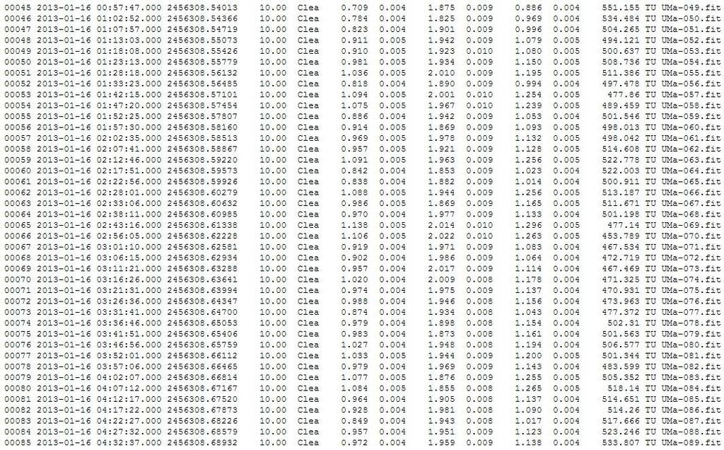
72 71

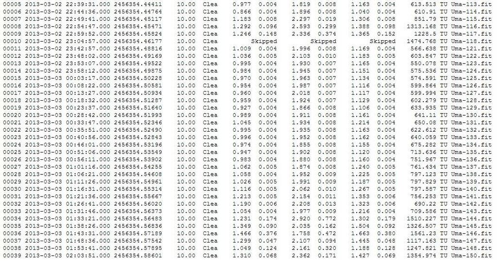
73 72

74 D Appendix 4 73

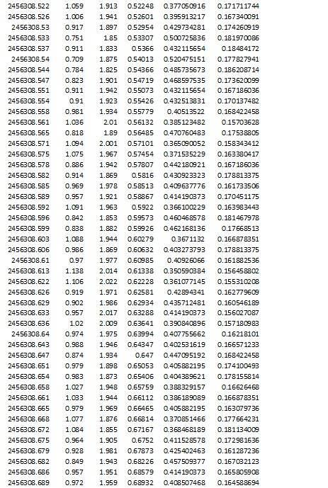
75 74

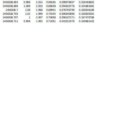
76 75

77 E Appendix 5 Meetings 7/12/12 Met with Graham Bryant to discuss aims of the project and identify possible stars, also considered an outline for the project 14/12/12 We chose our target star (TU UMa*) and used Stellarium to check the star 76