Chapter. Numerically Summarizing Data. Copyright 2013, 2010 and 2007 Pearson Education, Inc.

Transcription

1 Chapter 3 Numerically Summarizing Data

2 Section 3.1 Measures of Central Tendency

3 Objectives 1. Determine the arithmetic mean of a variable from raw data 2. Determine the median of a variable from raw data 3. Explain what it means for a statistic to be resistant 4. Determine the mode of a variable from raw data 3-3

4 Objective 1 Determine the Arithmetic Mean of a Variable from Raw Data 3-4

5 The arithmetic mean of a variable is computed by adding all the values of the variable in the data set and dividing by the number of observations. 3-5

6 The population arithmetic mean, μ (pronounced mew ), is computed using all the individuals in a population. The population mean is a parameter. 3-6

7 The sample arithmetic mean, x (pronounced x-bar ), is computed using sample data. The sample mean is a statistic. 3-7

8 If x 1, x 2,, x N are the N observations of a variable from a population, then the population mean, µ, is x 1 x 2 L x N N x i N 3-8

9 If x 1, x 2,, x n are the n observations of a variable from a sample, then the sample mean,, is x x x 1 x 2 L x n n x i n 3-9

10 EXAMPLE Computing a Population Mean and a Sample Mean The following data represent the travel times (in minutes) to work for all seven employees of a start-up web development company. 23, 36, 23, 18, 5, 26, 43 (a) Compute the population mean of this data. (b)then take a simple random sample of n = 3 employees. Compute the sample mean. Obtain a second simple random sample of n = 3 employees. Again compute the sample mean. 3-10

11 EXAMPLE (a) Computing a Population Mean and a Sample Mean x i N x x... x minutes 3-11

12 EXAMPLE Computing a Population Mean and a Sample Mean (b) Obtain a simple random sample of size n = 3 from the population of seven employees. Use this simple random sample to determine a sample mean. Find a second simple random sample and determine the sample mean. Let the random sample be 5,36 and 26. x Let the second random sample be 36,23 and 26. x

13 Objective 2 Determine the Median of a Variable from Raw Data 3-13

14 The median of a variable is the value that lies in the middle of the data when arranged in ascending order. We use M to represent the median. 3-14

15 Steps in Finding the Median of a Data Set Step 1 Arrange the data in ascending order. Step 2 Determine the number of observations, n. Step 3 Determine the observation in the middle of the data set. 3-15

16 Steps in Finding the Median of a Data Set If the number of observations is odd, then the median is the data value exactly in the middle of the data set. That is, the median is the observation that lies in then (n + 1)/2 position. If the number of observations is even, then the median is the mean of the two middle observations in the data set. That is, the median is the mean of the observations that lie in the n/2 position and the n/2 + 1 position. 3-16

17 EXAMPLE Computing a Median of a Data Set with an Odd Number of Observations The following data represent the travel times (in minutes) to work for all seven employees of a start-up web development company. 23, 36, 23, 18, 5, 26, 43 Determine the median of this data. Step 1: 5, 18, 23, 23, 26, 36, 43 Step 2: There are n = 7 observations. n Step 3: 4 M = , 18, 23, 23, 26, 36,

18 EXAMPLE Computing a Median of a Data Set with an Even Number of Observations Suppose the start-up company hires a new employee. The travel time of the new employee is 70 minutes. Determine the median of the new data set. 23, 36, 23, 18, 5, 26, 43, 70 Step 1: 5, 18, 23, 23, 26, 36, 43, 70 Step 2: There are n = 8 observations. n Step 3: 4.5 M , 18, 23, 23, 26, 36, 43, 70 M minutes 3-18

19 A numerical summary of data is said to be resistant if extreme values (very large or small) relative to the data do not affect its value substantially. 3-19

20 EXAMPLE Computing a Median of a Data Set with an Even Number of Observations The following data represent the travel times (in minutes) to work for all seven employees of a start-up web development company. 23, 36, 23, 18, 5, 26, 43 Suppose a new employee is hired who has a 130 minute commute. How does this impact the value of the mean and median? Mean before new hire: 24.9 minutes Median before new hire: 23 minutes Mean after new hire: 38 minutes Median after new hire: 24.5 minutes 3-20

21 EXAMPLE Computing a Median of a Data Set with an Even Number of Observations The following data represent the travel times (in minutes) to work for all seven employees of a start-up web development company. 23, 36, 23, 18, 5, 26, 43 Suppose a new employee is hired who has a 130 minute commute. How does this impact the value of the mean and median? Mean before new hire: 24.9 minutes Median before new hire: 23 minutes Mean after new hire: 38 minutes Median after new hire: 24.5 minutes Median is resistant whereas Mean is not resistant. 3-21

22 3-22

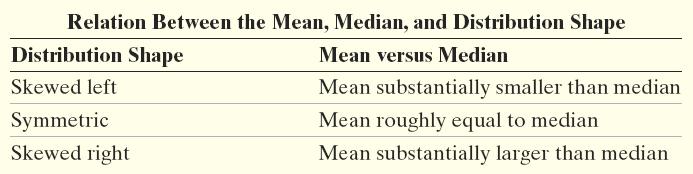
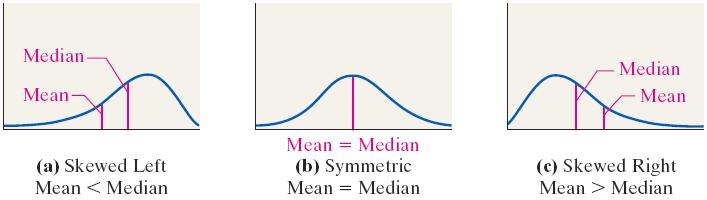
23 EXAMPLE Describing the Shape of the Distribution The following data represent the asking price of homes for sale in Lincoln, NE. 79, , , ,900 99, , , , , , , , , , , , , , , , , , , , , , , , , , , ,900 Source:

24 Find the mean and median. Use the mean and median to identify the shape of the distribution. Verify your result by drawing a histogram of the data. 3-24

25 Find the mean and median. Use the mean and median to identify the shape of the distribution. Verify your result by drawing a histogram of the data. The mean asking price is $168,320 and the median asking price is $148,700. Therefore, we would conjecture that the distribution is skewed right. 3-25

26 12 Asking Price of Homes in Lincoln, NE 10 8 Frequency Asking Price

27 Objective 4 Determine the Mode of a Variable from Raw Data 3-27

28 The mode of a variable is the most frequent observation of the variable that occurs in the data set. A set of data can have no mode, one mode, or more than one mode. If no observation occurs more than once, we say the data have no mode. 3-28

29 EXAMPLE Finding the Mode of a Data Set The data on the next slide represent the Vice Presidents of the United States and their state of birth. Find the mode. 3-29

30 Joe Biden Pennsylvani a 3-30

31 3-31

32 The mode is New York. 3-32

33 Tally data to determine most frequent observation 3-33

34 Section 3.2 Measures of Dispersion

35 Objectives 1. Determine the range of a variable from raw data 2. Determine the standard deviation of a variable from raw data 3. Determine the variance of a variable from raw data 4. Use the Empirical Rule to describe data that are bell shaped 5. Use Chebyshev s Inequality to describe any data set 3-35

36 To order food at a McDonald s restaurant, one must choose from multiple lines, while at Wendy s Restaurant, one enters a single line. The following data represent the wait time (in minutes) in line for a simple random sample of 30 customers at each restaurant during the lunch hour. For each sample, answer the following: (a) What was the mean wait time? (b) Draw a histogram of each restaurant s wait time. (c ) Which restaurant s wait time appears more dispersed? Which line would you prefer to wait in? Why? 3-36

37 Wait Time at Wendy s Wait Time at McDonald s

38 (a) The mean wait time in each line is 1.39 minutes. 3-38

39 (b) 3-39

40 Objective 1 Determine the Range of a Variable from Raw Data 3-40

41 The range, R, of a variable is the difference between the largest data value and the smallest data values. That is, Range = R = Largest Data Value Smallest Data Value 3-41

42 EXAMPLE Finding the Range of a Set of Data The following data represent the travel times (in minutes) to work for all seven employees of a start-up web development company. Find the range. 23, 36, 23, 18, 5, 26, 43 Range = 43 5 = 38 minutes 3-42

43 Although Range is easy to compute, it is sensitive to outliers. 3-43

44 The population standard deviation of a variable is the square root of the sum of squared deviations about the population mean divided by the number of observations in the population, N. That is, it is the square root of the mean of the squared deviations about the population mean. The population standard deviation is symbolically represented by σ (lowercase Greek sigma). 3-44

45 x 1 x i 2 N 2 x 2 2 L x N N 2 where x 1, x 2,..., x N are the N observations in the population and μ is the population mean. 3-45

46 A formula that is equivalent to the one on the previous slide, called the computational formula, for determining the population standard deviation is x i 2 x 2 i N N 3-46

47 EXAMPLE Computing a Population Standard Deviation The following data represent the travel times (in minutes) to work for all seven employees of a startup web development company. 23, 36, 23, 18, 5, 26, 43 Compute the population standard deviation of this data. 3-47

48 x i μ x i μ (x i μ) x 2 i x i 2 N minutes 3-48

49 Using the computational formula, yields the same result. x i (x i ) Σ x i = 174 Σ (x i ) 2 = 5228 x i 2 x 2 i N N minutes 3-49

50 The sample standard deviation, s, of a variable is the square root of the sum of squared deviations about the sample mean divided by n 1, where n is the sample size. s x i x 2 n 1 x 1 x 2 x 2 x n 1 2 L x n x 2 where x 1, x 2,..., x n are the n observations in the sample and x is the sample mean. 3-50

51 A formula that is equivalent to the one on the previous slide, called the computational formula, for determining the sample standard deviation is s x i 2 x 2 i n 1 n 3-51

52 The sum of deviations from the mean equal zero. We call n - 1 the degrees of freedom because the first n - 1 observations have freedom to be whatever value they wish, but the n th value has no freedom. It must be whatever value forces the sum of the deviations about the mean to equal zero. 3-52

53 EXAMPLE Computing a Sample Standard Deviation Here are the results of a random sample taken from the travel times (in minutes) to work for all seven employees of a start-up web development company: 5, 26, 36 Find the sample standard deviation. 3-53

54 x i x x i x x i x x i x s x i x 2 n minutes 3-54

55 Using the computational formula, yields the same result. x i (x i ) Σ x i = 67 Σ (x i ) 2 = 1997 x i 2 x 2 i n n minutes 3-55

56 EXAMPLE Comparing Standard Deviations Determine the standard deviation waiting time for Wendy s and McDonald s. Which is larger? Why? 3-56

57 Wait Time at Wendy s Wait Time at McDonald s

58 EXAMPLE Comparing Standard Deviations Sample standard deviation for Wendy s: minutes Sample standard deviation for McDonald s: minutes Recall from earlier that the data is more dispersed for McDonald s resulting in a larger standard deviation. 3-58

59 Objective 3 Determine the Variance of a Variable from Raw Data 3-59

60 The variance of a variable is the square of the standard deviation. The population variance is σ 2 and the sample variance is s

61 EXAMPLE Computing a Population Variance The following data represent the travel times (in minutes) to work for all seven employees of a start-up web development company. 23, 36, 23, 18, 5, 26, 43 Compute the population and sample variance of this data. 3-61

62 EXAMPLE Computing a Population Variance Recall that the population standard deviation is σ = so the population variance is σ 2 = and that the sample standard deviation is s = 15.82, so the sample variance is s 2 =

63 Note that Standard deviation has same unit of measurement as the variable whereas Variance has different unit. So, if the variable is measured in dollars, the variance is measured in dollars squared. This makes interpreting the variance difficult. However, the variance is important for conducting certain types of statistical inference, which we discuss later. Standard deviation and variance are sensitive to outliers. Standard deviation can be used in conjunction with the mean to describe the variability in a single data set. 3-63

64 Objective 4 Use the Empirical Rule to Describe Data that are Bell Shaped 3-64

65 The Empirical Rule If a distribution is roughly bell shaped, then Approximately 68% of the data will lie within 1 standard deviation of the mean. That is, approximately 68% of the data lie between μ 1σ and μ + 1σ. Approximately 95% of the data will lie within 2 standard deviations of the mean. That is, approximately 95% of the data lie between μ 2σ and μ + 2σ. 3-65

66 The Empirical Rule If a distribution is roughly bell shaped, then Approximately 99.7% of the data will lie within 3 standard deviations of the mean. That is, approximately 99.7% of the data lie between μ 3σ and μ + 3σ. Note: We can also use the Empirical Rule based on sample data with x used in place of μ and s used in place of σ. 3-66

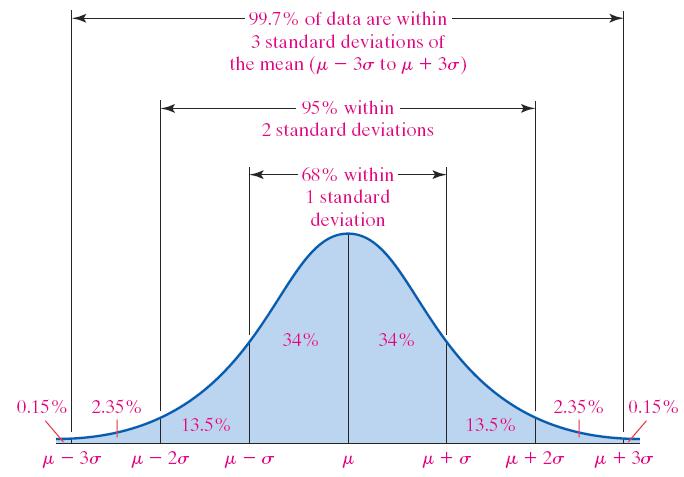
67 3-67

68 EXAMPLE Using the Empirical Rule The following data represent the serum HDL cholesterol of the 54 female patients of a family doctor

69 (a) Compute the population mean and standard deviation. (b) Draw a histogram to verify the data is bell-shaped. (c) Determine the percentage of all patients that have serum HDL within 3 standard deviations of the mean according to the Empirical Rule. (d) Determine the percentage of all patients that have serum HDL between 34 and 69.1 according to the Empirical Rule. (e) Determine the actual percentage of patients that have serum HDL between 34 and

70 (a) Using a TI-83 plus graphing calculator, we find (b) 57.4 and

71 (c) According to the Empirical Rule, 99.7% of the all patients that have serum HDL within 3 standard deviations of the mean. (d) 13.5% + 34% + 34% = 81.5% of all patients will have a serum HDL between 34.0 and 69.1 according to the Empirical Rule. (e) 45 out of the 54 or 83.3% of the patients have a serum HDL between 34.0 and

72 Objective 5 Use Chebyshev s Inequality to Describe Any Set of Data 3-72

73 Chebyshev s Inequality For any data set or distribution, at least 1 1 k 2 100% of the observations lie within k standard deviations of the mean, where k is any number greater than 1. That is, at least 1 1 of the data lie between μ kσ k 2 100% and μ + kσ for k > 1. Note: We can also use Chebyshev s Inequality based on sample data. 3-73

74 EXAMPLE Using Chebyshev s Theorem Using the data from the previous example, use Chebyshev s Theorem to (a) determine the percentage of patients that have serum HDL within 3 standard deviations of the mean % 88.9% (b) determine the actual percentage of patients that have serum HDL between 34 and 80.8 (within 3 SD of mean). 52/ % 3-74