Universal time effect in the response of the thermosphere to electric field changes

Transcription

1 JOURNAL OF GEOPHYSICAL RESEARCH, VOL.???, XXXX, DOI: /, 1 2 Universal time effect in the response of the thermosphere to electric field changes N. J. Perlongo, 1 A. J. Ridley, 1 Corresponding author: Nick Perlongo, Department of Atmospheric, Oceanic, and Space Sciences, University of Michigan, Ann Arbor, Michigan, USA. (nperlong@umich.edu) 1 Department of Atmospheric, Oceanic, and Space Sciences, University of Michigan, Ann Arbor, Michigan, USA. This is the author manuscript accepted for publication and has undergone full peer review but has not been through the copyediting, typesetting, pagination and proofreading process, which may lead to differences between this version and the Version of Record. Please cite this article as doi: D R /2015JA A F T April 6, 2016, 3:49am D R A F T

2 3 X - 2 Abstract. PERLONGO ET AL.: THERMOSPHERE UT EFFECTS Understanding the dynamics of the thermospheric mass den sity is of paramount importance for predicting drag on low altitude satellites, particularly during geomagnetic storms. Transient enhancements in ion velocities, which frequently occur as a result of storm-driven solar wind electric field fluctuations, cause increases in neutral density and temperature. Since the Earth s quasi-dipolar magnetic field is tilted and offset from the center of the planet, it is hypothesized that hemispheric asymmetries arise, altering the thermospheric response to energy input based upon the time of day. This study used the Global Ionosphere-Thermosphere Model (GITM) to investigate this phenomenon via a series of 22 idealized simulations, where the convective electric field was enhanced for one hour of the day. Two configurations of the Earth s magnetic field were considered, the International Geomagnetic Reference Field (IGRF) and a centered dipole. These runs were conducted at March equinox when the amount of sunlight falling on the two hemispheres was the same. Two additional sets of runs were conducted at the June and December solstices for comparison. It was found that the most geo-effective times were those times when the geomagnetic poles were pointed towards the sun. This orientation maximizes the photoionization co-located with the high-latitude potential pattern, leading to more in Joule heating.

3 PERLONGO ET AL.: THERMOSPHERE UT EFFECTS X Introduction Understanding the thermospheric response to energy input is important for the practical reason that as energy is added to the system, the thermosphere expands and causes more drag on low altitude satellites [Bruinsma et al., 2006; Zhou et al., 2009]. The accuracy of accelerometer derived thermospheric densities and winds has improved in recent years [e.g. Sutton et al., 2007; Sutton, 2009], making it possible to examine the disturbed and 27 quiescent state of the thermosphere. For example, Ritter et al. [2010] found that the polar thermospheric density increased by 4-15% during substorms, depending on the level of geomagnetic activity. Furthermore, satellite observations have unveiled seasonal and local time dependence of the thermospheric density [Hedin and Carignan, 1985; Bruinsma et al., 2006; Rentz and Lühr, 2008; Müller et al., 2009]. The influence of magnetospheric electric fields on the thermosphere is intricately tied 33 to the plasma motion, as well as the density and velocity of the neutrals. Therefore magnetospheric electric fields are a crucial process when considering any possible UT effects. The thermospheric energy balance is strongly coupled to the ionosphere through 36 the difference between ion and neutral velocities. The time-scale of velocity changes in the ions is significantly shorter than in the neutrals [Vasyliunas, 2005]. This means that the ion flows across the field-lines are relatively weakly controlled by the neutrals [Deng et al., 1991; Odom et al., 1997], but the neutral flows across the field lines are more strongly controlled by the ion flows [Deng, 2006; Conde and Smith, 1995; Mikkelsen et al., 1981]. Consequently, the magnetic field direction is important for controlling both the ion flows and the neutral winds. In addition, the component of the neutral wind along the

4 X - 4 PERLONGO ET AL.: THERMOSPHERE UT EFFECTS magnetic field can strongly control the structure of the ionosphere - when the magnetic field is oriented between the horizontal and vertical directions, neutral winds can push plasma along the field lines [Bramley and Young, 1968; Burrell et al., 2012, 2013], causing the height of the F 2 peak to move up or down, depending on the structure of the wind and magnetic field [Hedin and Mayr, 1973; Rishbeth et al., 1978; Rishbeth and Mendillo, 2001; Muella et al., 2010]. The Earth s quasi-dipolar field is both tilted and offset from the center of the planet. This means that there are large asymmetries in the geomagnetic field, both between the poles and in the equatorial region [Shepherd, 2014]. In addition, there are crustal fields that locally modify the magnetic field [Mandea and Purucker, 2005]. The location of the geomagnetic pole in each hemisphere controls where magnetospheric electric fields and auroral particles deposit energy into the thermosphere. For example, regions of energetic particle precipitation roughly vary in accordance with convection and potential patterns [Foster et al., 1986; Singh et al., 2013; Mitchell et al., 2013], the location of which are heavily influenced by the location of the Earth s geomagnetic pole. The International Geomagnetic Reference Field (IGRF) [Finlay et al., 2010] has determined the geographic location of the northern geomagnetic poles to be latitude and longitude, and the southern at latitude and longitude, in The response of the ionosphere/thermosphere system to impulsive events may be strongly dependent upon the time of the event, because the Earth s geomagnetic field rotates through the Sun-fixed coordinate system. When the geomagnetic pole is in sunlight, there is more ion production in regions of strong electric potential, such as the throat. In this case, the Joule heating that results from a difference in the ion and neutral

5 PERLONGO ET AL.: THERMOSPHERE UT EFFECTS X velocities may be stronger. Therefore, the thermospheric response to solar wind and interplanetary magnetic field changes may be dependent upon universal time (UT). Because the geomagnetic pole is offset from the Earth s rotational axis, the magnetospheric energy is deposited in different locations relative to the solar terminator. Such UT modulation may be larger in the southern hemisphere, because the greater separation between geographic and geomagnetic poles [Fuller-Rowell et al., 1988] causes the geomagnetic pole to be at lower solar zenith angles during the day and higher solar zenith angles at night. It is well known that the magnetospheric activity level is dependent upon the time of day and season, because of the tilt of the geomagnetic pole away from Earth s rotation axis [Russell and McPherron, 1973]. This so-called Russell-McPherron effect occurs because if one takes the nominal interplanetary magnetic field (IMF) as being in a Parker spiral (i.e., B y being roughly opposite of B x, and B z being approximately zero) and the field is transformed from GSE to GSM coordinates in which the Z-axis is oriented in the plane of the magnetic field axis, instead of the equatorial plane of the sun, GSM B z gains some magnitude from GSE B y. This means that there will be time periods of negative GSM B z when the IMF is actually a pure Parker spiral in GSE coordinates, and implies that there may be a larger amount of activity for nominal solar wind and IMF conditions during the equinoxes when this geometry maximizes [Russell and McPherron, 1973; Liou et al., 2001]. In addition to the Russell-McPherron effect, seasonal variations have also been found to be caused by variations in the angle between the geomagnetic dipole axis and the solar wind flow direction [Cliver et al., 2000]. Furthermore, UT variations as a result of magnetosphere-solar wind coupling have been reproduced in numerical model simulations,

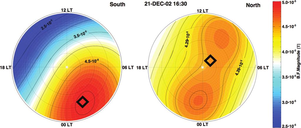
6 X - 6 PERLONGO ET AL.: THERMOSPHERE UT EFFECTS primarily through changes in the magnetic reconnection process [Cnossen et al., 2012]. In this study, we primarily examined what the thermospheric effects are due to the same 91 change in high-latitude drivers, but at different times of the day. While these effects are influenced by the tilt of the dipole, this study examined the ramifications of the northern and southern geomagnetic poles being at different solar local times, and what this means for ionosphere/thermosphere coupling, rather than the magnetosphere/solar wind coupling. Longitudinal variations in the strength of Earth s magnetic field strength can also contribute to UT variations [Förster and Cnossen, 2013; Cnossen et al., 2012]. The magnetic field magnitudes are shown for each hemisphere in Figure 1. Each plot shows the magnitude at 1700 UT poleward of 50 latitude at 590 km altitude. The two peak structure in the northern hemisphere differs greatly in comparison to the larger single peak structure in the southern hemisphere. One can imagine these structures rotating in local time throughout the day. This rotation alters the local magnetic field strength on the dayside, causing significant changes in the electric current and ion drift in the ionosphere, as well as ion drag in the thermosphere [Rees and Fuller-Rowell, 1989]. The magnetic field strength has also been found to alter the height F 2 peak of the ionosphere [Cnossen et al., 2012; Sojka and Schunk, 1997], which could translate into a UT dependence based on the longitudinal variation described in Figure 1. Longitudinal variations in the electron density have also been found recently. Zonal winds were found to be responsible for up to 80% of the longitudinal variations in electron density during equinox in a series of Global Ionosphere Thermosphere Model (GITM) simulations [Wang et al., 2015]. Additionally, the ionosphere response to storms in the American sector in the afternoon was found to

7 PERLONGO ET AL.: THERMOSPHERE UT EFFECTS X be larger in terms of total plasma content [Immel and Mannucci, 2013; Garner et al., 2010]. The effect of a weaker dipole on the ionosphere/thermosphere system was investigated recently by Cnossen et al. [2011]. By reducing Earth s dipole moment by 25% in their simulations, they found that Joule heating power (Joule heating integrated both hemispherically and in height) was increased by a minimum of 13% in the northern hemisphere summer, and a maximum of 30% for March equinox in the southern hemisphere. Since the potential pattern rotates with the geomagnetic pole, the average magnetic field strength in the throat region of the potential pattern varies throughout the day. The idea of a UT dependence in the ionosphere/thermosphere system is not new. Numerical simulations to investigate how magnetospheric activity can produce a UT effect in a global thermospheric circulation model were done decades ago [Roble et al., 1982; Fesen et al., 1995]. These early studies found that maximum perturbations in each hemisphere occur 12 hours offset from each other. Fuller-Rowell et al. [1994] also performed numerical simulations using a coupled ionosphere/thermosphere model where they found the atmospheric response to depend on the longitude of the geomagnetic pole. Despite the interest over the last few decades, the particular mechanics of this UT dependence and the magnitude of its effects are still not completely understood. This study aims to improve that understanding by looking at changes in thermospheric temperature, as well as neutral and electron densities caused by an idealized change in the interplanetary magnetic field.

8 X - 8 PERLONGO ET AL.: THERMOSPHERE UT EFFECTS 2. Technique This study used GITM, a model that is described in detail by Ridley et al. [2006]. It is a three dimensional model that solves the continuity, momentum, and energy equations with realistic source terms in a spherical coordinate system. A primary difference between GITM and other ionosphere/thermosphere models is that GITM uses an altitude grid, instead of pressure, which facilitats the ability to develop non-hydrostatic solutions. GITM was run with a resolution of 2.5 latitude by 5 longitude with a stretched altitude, resolving the vertical scales to approximately 1/3 of a scale height. Idealized simulations were used to obtain an understanding and quantifiable estimate of how important UT effects are for the response of the ionosphere/thermosphere system to impulsive events. GITM was run for 48 hours prior to any changes in the drivers to eliminate any transient influence of the initial conditions. 23 simulations were then continued from the startup simulation and run for 24 hours from March 21 st 0000 UT. 22 of these simulations were disturbed by changing the high latitude electric potential for 70 minutes. This was accomplished by using the Weimer [2005] electric potential model, and altering the IMF B z component (in GSM coordinates) from 2 nt to 10 nt linearly over ten minutes, holding the IMF B z constant at 10 nt for 50 minutes, then linearly changing the IMF B z back to 2 nt over ten minutes. IMF B y and B x were held at zero. It is important to note that the use of the Weimer empirical electric potential model implicitly includes the UT variations resulting from solar wind/magnetosphere coupling, due to the tilt angle dependence. To illustrate this, the cross polar cap potential (CPCP) for the baseline equinox simulation is plotted in Figure 2. The CPCP is calculated by taking the difference between the maximum and minimum electric potentials in each

9 PERLONGO ET AL.: THERMOSPHERE UT EFFECTS X hemisphere. The plot shows a UT variation in both hemispheres. However, since the amplitude of this variation is only about 2 kv, the overall effect in the thermosphere response will be minimal relative to the magnitude of the idealized energy input event. The perturbed CPCP reaches values of about 160 kv (not shown), so the UT variation only comprises a couple of percent of the large perturbation. There were no changes in any other solar wind drivers, auroral specifications, or solar extreme ultraviolet (EUV) inputs. The F 10.7 for this series of runs was fixed at 100 sfu (solar flux units), while the auroral hemispheric power was held constant at 20 GW. While it is relatively unphysical to have no change in aurora with a strong change in the ionospheric electric field, it could be viewed as a time period of steady magnetospheric convection in which a substorm does not occur [DeJong et al., 2008; DeJong, 2014; Newell et al., 2010]. The only difference between the 22 different runs was the time in which the change in IMF B z occurred - each run was offset by one hour from the previous run. In other words, run 1 had the start of the IMF transition start occurring at 0100 UT and the perturbation ending at 0210 UT, run 2 had the transition occurring at 0200 UT and ending at 0310 UT, and so on. The 23 rd simulation had no IMF change at all and was the reference simulation. The IGRF was used in all simulations, except when noted. Since the IGRF model was used, effects from magnetic field strength and tilt angle variations with longitude are expected. In a second series of 23 runs, the magnetic field was set to a pure dipole in which the magnetic and geographic axes were aligned. These simulations serve to eliminate both the tilt angle effect and longitudinal variations in magnetic field strength. The Mass Spectrometer and Incoherent Scatter (MSIS) model [Hedin, 1991]

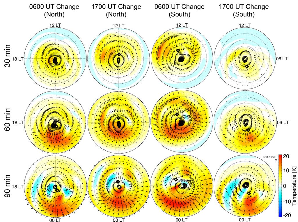
10 X - 10 PERLONGO ET AL.: THERMOSPHERE UT EFFECTS was used as a lower boundary at 97 km, which also introduced atmospheric tides to the simulation results as well. 3. Results and Discussion Figures 3 and 4 show simulation results of the temperature and winds in the northern and southern hemispheres from two of the runs (the 0600 UT and 1700 UT change times) during and after the period of the electric potential perturbation. These plots show the difference between the perturbed run and the baseline case, which was run with a constant IMF Bz. or the purposes of this discussion, time (t) 0 min refers to the onset time of the perturbation for a particular run, with subsequent times indicating the number of minutes after the onset of the perturbation. While all of the patterns for the same time are very roughly similar to each other, the hemispheres and simulations where the geomagnetic pole (indicated by a diamond on each plot) is on the same side of the terminator when the electric field change occurred show stronger congruency. Since these simulations were run at equinox, the terminator lies along the line from 0600 UT to 1800 UT, with the day side being on the top half of each plot. The difference between the daytime and nighttime response can be seen by comparing either the 1700 UT north and 0600 UT south plots (central two columns, in which the geomagnetic pole was on the dayside) or the 0600 UT north and 1700 UT south plots (outer two columns, in which the geomagnetic pole was on the nightside). At t=30 (first row), the neutral winds were enhanced in all simulations. Each plot shows a two cell convection pattern, which is similar to the ion convection at the time (not shown). In addition, the temperature had increased in each simulation with a somewhat similar pattern. This is the general pattern that one expects from a Joule

11 PERLONGO ET AL.: THERMOSPHERE UT EFFECTS X heating enhancement in the high latitude region [e.g. Thayer, 1998; Zhang et al., 2005; Immel et al., 2006; Deng and Ridley, 2007]. In each of the time-series, the thermosphere heated up when the electric field increase was applied (at t=30 and t=60), and then cooled down afterwards (from t=90 onward). The cooling completed a clear wave-like structure that propagated away from the polar region, which can be observed by following a single hemispheric simulation through Figures 3 and 4. For example, in the second and third columns, there was a temperature peak on the nightside at 65 latitude at t=90. This peak moved to 55 latitude by t=120 and 45 latitude at t=150 on the nightside. This roughly corresponds to a wave speed of 620 ms 1, while the sound speed was close to 875 ms 1. Previous model results have found the phase speed of this global wind surge to be about 600 ms 1 as well [Fuller-Rowell et al., 1994]. Associated with this wave were equatorward perturbations in the winds in excess of 200 ms 1. These perturbed winds lasted until t=120, when they started decreasing and rotating in the westward direction, as one might expect due to the Coriolis force. By 210 minutes after the start of the enhancement, the temperature had decreased over almost the entire polar region and the large equatorward winds had less than half of their peak perturbed values. On the dayside in the inner columns, the temperature increased from the pole to 50 at 30 minutes. It then expanded to below 40 latitude before 60 minutes. At that time, there was a significant equatorward flow perturbation on the dayside at low latitudes, while there was little equatorward flow perturbation on the nightside at such low latitudes. The equatorward flow on the dayside decreased rapidly and by t=120, the main flow was poleward near noon, due to the residual ion drag driven by the two-cell convection pattern.

12 X - 12 PERLONGO ET AL.: THERMOSPHERE UT EFFECTS This two-cell pattern remained for at least two hours after the electric field enhancement had ended, although it became quite distorted as it rotated with the planet. When the enhancement happened while the magnetic field was on the night side (the outer two columns), the initial perturbation was more confined and was smaller in magnitude. Additionally, the disturbance did not extend on to the dayside nearly as much as the nightside. Also, the resulting wind perturbations were also much weaker than when the enhancement occurred while the geomagnetic pole was on the dayside. The effects on the thermospheric mass density were also explored, though they are not shown. At 404 km, the general behavior of the simulated density was very similar to the behavior observed in the temperature plots in Figures 3 and 4, though the impact was more severe. While the temperature scale went up to 25% at 404 km altitude, the mass density scale went up to about 100%, indicating that the heating occurred significantly lower than 404 km and that the atmosphere was being lifted by the heating that occurred [Deng et al., 2013]. It should be noted that some of the differences between the hemispheres in Figures 3 and 4 may be attributed to plotting in the geographic coordinate system, while the driving is controlled in the magnetic coordinate system. The following figures show a more hemispherically integrated perspective, but it is still possible that some hemispheric asymmetries appear from displaying results geographically, when many of the physical processes at hand are more oriented towards a magnetic coordinate system. While switching to a geomagnetic system may change the structuring of the peaks and valleys, it would not change the magnitude of the changes.

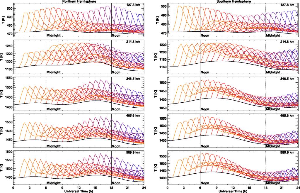
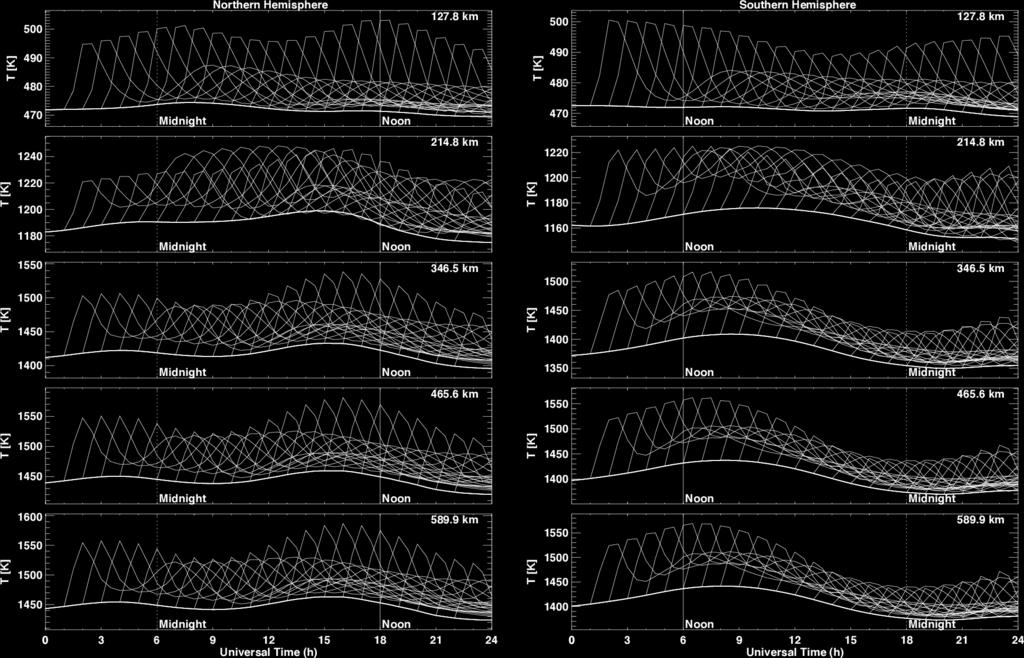
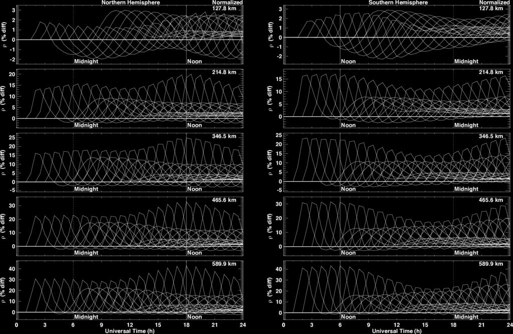
13 PERLONGO ET AL.: THERMOSPHERE UT EFFECTS X The plots in Figure 5 show the average temperature poleward of 45 geographic latitude for the northern and southern hemispheres, plotted on the left and right respectively. The black line shows the unperturbed baseline simulation, while the 22 colored lines show the results of the 22 simulations where the electric field perturbation started at 0100, 0200, 0300,..., 2200 UT, and started to end at 0200, 0300, 0400,..., 23 UT00. The get darker with the time of the perturbation. Five altitudes are plotted, starting at 128 km altitude at the top and going to 590 km on the bottom. If a single color trace is followed, the heating during the IMF enhancement is observed, encompassing the changes shown in Figures 3 and 4. The temperature is observed to increase rapidly during the perturbation in IMF, peaking at one hour, which is the time when the IMF started to recover back to its nominal value. The thermosphere then rapidly cooled. A minimum in temperature was reached around 4.5 hours after the start of the enhancement. Shortly after this, the gravity wave (or travelling atmospheric disturbance) from the opposite hemisphere entered the polar region and the temperature started to increase again, warming to a point just a few degrees cooler than the highest temperature peak. The secondary peak temperature was reached about 9 hours after the start of the electric field enhancement. This is consistent with a wave propagating at 620 ms 1, as discussed earlier (i.e., it traveled roughly from pole to pole in nine hours). All of the traces have similar behavior - a quick rise, slower decay and secondary maximum about nine hours later, though this is only visible for the first few simulations. The temperature oscillated for the rest of the simulation, but overall trended towards the background simulation temperature. The magnitude of the perturbations in Figure 5 is dependent on the altitude and the time of day. The largest temperature increases at each altitude spanned 31K at 126

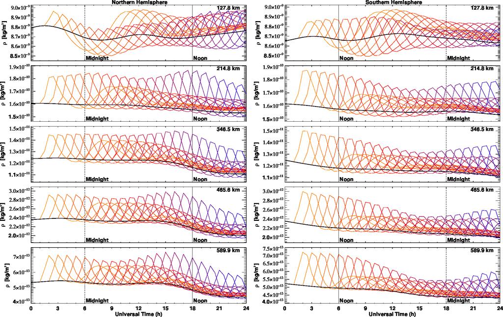
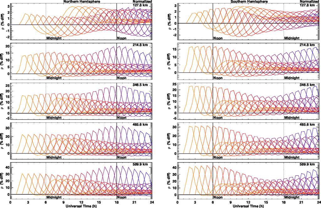
14 X - 14 PERLONGO ET AL.: THERMOSPHERE UT EFFECTS 266 km, to 122K at 590 km. Comparing temperature enhancements that occurred when the geomagnetic pole was closer to noon to those when the geomagnetic pole was closer to midnight suggests a dependence on UT. For example, at 590 km in the southern hemisphere, the temperature increased by 129K when the geomagnetic pole was near noon, but only 68K when the pole was near midnight. In the northern hemisphere, the UT variation was smaller, with the maximum perturbation at 590 km of 122K, and the minimum perturbation of 86K. The averaged high-latitude mass density perturbation was also dependent upon the 274 UT at which the electric field enhancement occurred (Figure 6). This was true at all altitudes and in both hemispheres, but was more apparent in the southern hemisphere. For example, at 590 km in the southern hemisphere, the density increase was kg m 3 when the geomagnetic pole was near midnight and kg m 3 when it was near noon. In the northern hemisphere the difference was slightly less. The maximum perturbation was the same as in the southern hemisphere, but the minimum perturbation reached kg m 3. The behavior seen in the simulations is easier to understand if the percentage differences between the perturbed and unperturbed simulation are explored, as shown in Figure 7. The figure shows the mass density perturbation values divided by the unperturbed simulation values, or ρ = 100(ρ p ρ u )/ρ u, where the mass density, ρ, is the value shown in each line, ρ p is the value of the perturbed simulation (colored lines in Figure 6), and ρ u is the mass density of the unperturbed run (black lines in Figure 6). Mass densities below the unperturbed simulation (negative percentage changes) resulted from the mass density

15 PERLONGO ET AL.: THERMOSPHERE UT EFFECTS X collapsing after the perturbation ended, leading to the natural negative well of a gravity wave. At high altitudes in the northern hemisphere, there was a weak increase in density (30% at 590 km) when the perturbation occurred in the first half of the day (in terms of UT) when the geomagnetic pole was on the nightside, but a more prominent increase (42% at 590 km) when the perturbation occurred later in the day when the geomagnetic pole was on the dayside. For the southern hemisphere, the larger perturbations occurred earlier in the day, with a 43% change occurring when the geomagnetic pole was near noon and a 23% change occurring when it was near midnight. At 215 km, 347 km, and 466 km, the structure of the differences remained the same, but the magnitude of the change increased with altitude. The noon-midnight difference shrank from 18% at 590 km to 4% at 215 km. In other words, the density perturbations were larger at higher altitudes when the geomagnetic pole was closer to noon. 301 The behavior at the lowest altitude was different than at the higher altitudes. The secondary peak in the wave structure at 128 km altitude was much stronger in both hemispheres. These peaks were often nearly 50% greater in the simulations near midnight. The magnitude by which this peak exceeded the initial perturbation was larger in the northern hemisphere by 0.5%. Interestingly, at 128 km altitude in the northern hemisphere, the perturbations around 1000 UT were primarily reductions, while around 2000 UT, the perturbations almost always increased. In the southern hemisphere at 128 km altitude, a similar behavior was observed, but the reductions took place towards the middle of the day, while the largest increases also tended to occur during the same time-

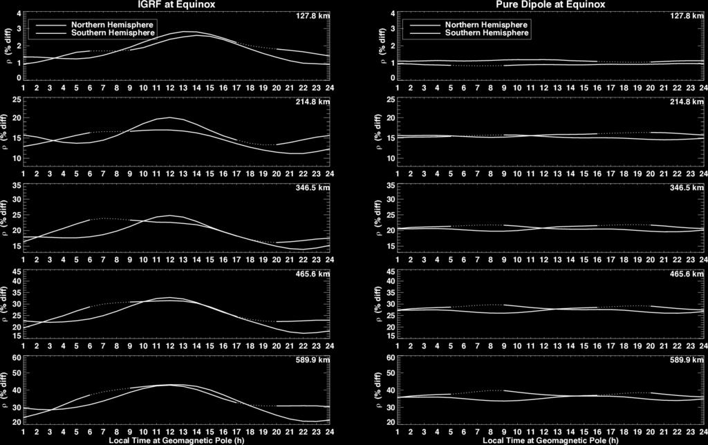
16 X - 16 PERLONGO ET AL.: THERMOSPHERE UT EFFECTS frame. Note that the percentage change at low altitudes was extremely small compared to the response at higher altitudes (1-3% versus about 20-45%, respectively). Variations in the trends in the lower and upper thermospheric mass density response may be due to different effects. For example, at lower altitudes, the tides may play a role [Groves and Forbes, 1984; Fesen et al., 1986]. At 120 km, the thermosphere is still dominated by tides from the lower atmosphere, while by 200 km, the thermosphere is more decoupled from the lower atmosphere tidal structures [Groves and Forbes, 1984]. It should be noted that even at F region heights, lower atmosphere tidal structures can still have important effects [Immel et al., 2006]. The perturbations caused by the IMF changes may have acted in or out of phase with the natural tidal structures. Additionally, oscillations generated by thermospheric winds below 200 km have been found to interact with lower atmospheric tides [Müller-Wodarg et al., 2001]. This interaction could modify the interference of the perturbation with the tidal structures. The prevalence of these tides in the GITM simulations are investigated further in Figure 9. Further, the Joule heating energy is typically deposited at altitudes between 110 and 150 km [Deng et al., 2011; Huang et al., 2012]. Therefore, the gradient in pressure may have decreased at the 128 km altitude slice, possibly causing downward flow, which would decrease the density. Figure 8 shows the local time variation of the averaged maximum thermospheric mass density perturbation over the polar region at the end of the IMF perturbation for both the southern and northern hemispheres. The lines in the left plots were derived by finding the maxima of the initial perturbations in the percentage change of the mass density as shown in Figure 7 (i.e., tracing from peak to peak). The lines were then shifted to correspond to the local time of the geomagnetic pole in each hemisphere. The dotted segments in each

17 PERLONGO ET AL.: THERMOSPHERE UT EFFECTS X curve represent missing simulations (i.e., IMF changes at 2300 and 0000 UT), which were filled in using a spline interpolation. The left plots in Figure 8 were derived directly from Figure 7, while the right plots were derived by re-running all of the simulations using an ideal dipole that was aligned with the rotation axis of the Earth. A strong local time dependence in the density response was seen in each hemisphere at all altitudes in the IGRF case. At most altitudes, the peak in density in each hemisphere corresponded to the time when the geomagnetic pole in that hemisphere was closest to noon, while the minimum occurred when the pole was close to midnight. The peaks for the southern hemisphere were broader than in the northern hemisphere, especially on the morning side. The density perturbation in the southern hemisphere was weaker from local time, but was stronger from local time. The weaker reaction at night may have been caused by the larger offset between the geographic and geomagnetic poles in the southern hemisphere. If this were true, one would expect a larger reaction at noon, which did not happen. It could be that the strength of the magnetic field or some other longitudinally dependent process could cause this difference, which is explored in more detail below. The magnitude of the percentage differences in mass density changes with altitude. Table 1 shows an overview of the maximum, minimum, and mean percentage changes at each altitude for the IGRF case shown in the left panel of Figure 8. Magnitudes range from a 1-3% increase at 128 km to a 22-43% increase at 590 km. In the pure dipole case, shown in the right panel of Figure 8, the northern and southern hemisphere density perturbations do not alter significantly with local time. This is what was expected during equinox for a dipole aligned with the rotation axis of the Earth, since there was no tilt or offset to create an asymmetry by which the UT of electric field

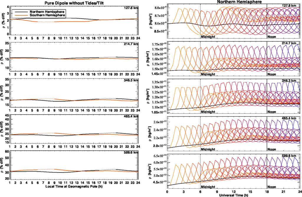
18 X - 18 PERLONGO ET AL.: THERMOSPHERE UT EFFECTS perturbation would make a difference. Note that since the geomagnetic and geographic poles are at the same location in the centered/pure dipole plots, the time here does not 358 exactly correspond to a local time at the geomagnetic pole. The local time shown in 359 the x-axis for these plots was calculated from the longitude of the geomagnetic pole in 360 the IGRF simulations. This aligns the same universal times with the other plots for better comparison. The difference between hemispheres may be attributed to tides, slight variations in the background thermosphere when the perturbation occurred, and a slight UT dependence in the Weimer [2005] model, or a combination of these influences. To investigate this, the pure dipole case was re-run with MSIS tides removed as well as 365 a 0 tilt specified for the potential model. Shown in Figure 9, this decreased the UT dependence at higher altitudes. The remaining dependence could be due to the short 2 day start-up time in all of the simulations, though we expect this to account for no more than a few percent of it. The simulations with the perturbations induced at the end of the day were introduced to an ionosphere/thermosphere system that was a couple percent 370 closer to steady state than the previous simulations. This interpretation is supported by the behavior of the baseline simulation from the run without tides or tilt shown in the right panel of Figure 9. At higher altitudes, the baseline simulation increases to a point before reaching steady state just after 1200 UT. However, Figure 12 will later show that this cannot fully explain the remaining UT dependence shown here. Interestingly, the times that the northern ( UT) and southern ( UT) hemispheres had the strongest perturbations in the dipole simulations were the same times that the strongest perturbations were seen in the IGRF simulations. Other studies have shown

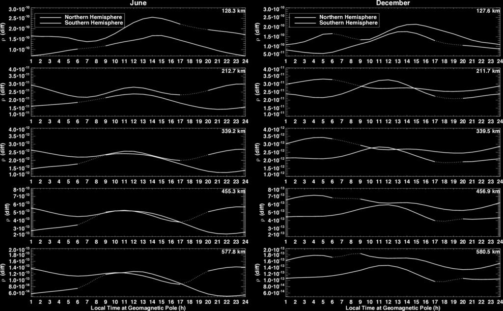
19 PERLONGO ET AL.: THERMOSPHERE UT EFFECTS X that the neutral wind response follows a similar response in each hemisphere during these times [Förster and Cnossen, 2013]. The previous series of runs were done for equinox conditions, but Figure 10 shows the same simulation results for the 22 simulations as shown in Figure 8 (left), but conducted for June (left) and December (right) solstice conditions. These simulations were run using the IGRF. In these simulations, the winter hemisphere had larger perturbations compared to the summer hemisphere case when the pole was near noon and a smaller perturbation 385 when the pole was near midnight. During the solstice, the winter hemisphere showed a strong dependence of the thermospheric response to the local time of the pole, while summertime in both hemispheres appeared to dampen the UT dependence in the mass density response to energy input. This seasonal dependence can be seen when comparing the northern hemisphere in the June and December simulations. In December, the largest perturbation in the northern hemisphere occurred near noon, while in June, the response was nearly semi-diurnal. The summer perturbations also had a small magnitude, peaking with nearly the same response at noon and midnight. This may be because the electron density variation that the pole is subjected to during the summer is smaller than at equinox or in the winter. The summer signature in the southern hemisphere was not symmetric around noon as it was in the northern hemisphere. At altitudes above 200 km, the density perturbations were largest near 0500 LT, and smallest near 1900 LT. Note that part of these asymmetries are due to the tilt angle dependence in the electric potential model, but that only accounts for a small percentage of the electric field variation throughout the day as seen in Figure 2. Furthermore, a relatively larger maximum to minimum difference in the perturbations

20 X - 20 PERLONGO ET AL.: THERMOSPHERE UT EFFECTS existed in the southern hemisphere winter in comparison to northern hemisphere winter. Table 2 summarizes the maximum percentage changes from Figure 10. The magnitude of the differences of the maxima compared with equinox conditions in Table 1 are within 3% of each other, but the southern hemisphere winter showed increasing divergence from the northern hemisphere winter as a function of altitude. There was a nearly 8% larger 406 response at 590 km in the southern hemisphere. A et al. [2012] also found that the 407 thermosphere density enhancements following a geomagnetic storm were greater in the 408 southern polar region, but only during vernal equinox. They noted that this may be explained by a weaker magnetic field, allowing for stronger ion flows and subsequent Joule heating. These results raise an interesting question regarding the seasonal dependence of the response of the thermosphere to electric field enhancements. If we expect the increased electron density in the summer polar cap to drive a stronger response in the temperature and neutral mass density, then why did the winter hemisphere show a stronger percentage change in Figure 10? The answer to this is partly revealed by looking at the absolute 416 differences in Figure 11. In December, altitudes above 340 km show a large absolute difference in the summer hemisphere for all local times. The larger percentage change in the winter hemisphere was therefore due to a less dense background thermosphere, not to a larger absolute change. However, the June results behave differently at similar altitudes. Here the summer hemisphere s response is only larger when the geomagnetic pole is near local midnight. The winter hemisphere s difference is just as large as the summer s when the southern geomagnetic pole is pointed towards the sun.

21 PERLONGO ET AL.: THERMOSPHERE UT EFFECTS X These asymmetries may be attributed to the larger diurnal change in the local magnetic field intensity. Figure 1 indicates that the structure of the magnetic field in the southern hemisphere lends itself to a potential pattern with a more varied background magnetic field strength throughout the day. Another way to explain the hemispheric asymmetry in the reaction is through the diurnal variation of the mean electron density in each hemisphere. Figure 12 shows the mean electron density above 50 magnetic latitude at an altitude of 346 km plotted against the local time of the geomagnetic pole for the 4 baseline simulations of each of the major run sets presented in this paper, as well as 2 additional simulations to investigate the importance of tides in the UT variation. Note that the plots in the top row have a jump in the electron density occurring around 1800 LT in the northern hemisphere and 0600 LT in the southern hemisphere. This corresponds to the change from the end of one day to the start of the same day 24 hours earlier, which indicates that these simulations are not fully in steady state. The first is the March equinox case using the IGRF magnetic field configuration in plot a. Here the electron density is more variable in the southern hemisphere. When the local time at the geomagnetic pole is closest to noon, the electron density in the southern hemisphere is greater than the northern hemisphere, but near midnight it is smaller. The degree of flatness in the peak surrounding local noon in the southern hemisphere resembles the neutral density peaks in Figure 8 above 200 km. Plot f of Figure 12 shows that the simulation with a centered dipole magnetic field configuration without atmospheric tides has no difference between hemispheres in electron density at all, which was expected. However, there is still a very small diurnal variation in both hemispheres, which may be due to a boundary condition or model parameter that has a

22 X - 22 PERLONGO ET AL.: THERMOSPHERE UT EFFECTS UT dependence not fully considered here. Interestingly, it appears that the introduction of tides in the model causes the simulation to take longer to reach steady state, as Plots d and f of Figure 12 have almost no jump, but Plots a-c, and e of Figure 12 do. The electron density results from the solstices are shown in Plots b and c of Figure 12. The winter hemisphere was characterized by a more prominent diurnal variation in electron density. In the southern hemisphere winter (dashed curve in Plot c of Figure 12), this effect was especially pronounced as the electron density reached a higher maximum and lower minimum than the northern hemisphere winter (solid line Plot b of Figure 12). This result has also been observed in topside electron density data from the Defense Meteorological Satellite Program (DMSP) [Garner et al., 2010]. The southern hemisphere winter electron density was also more symmetric around noon, similar to the neutral 457 density simulations in Figure 10. The electron density was nearly identical for each hemisphere in the summer, implying that as more of the hemisphere is covered in sunlight, the UT dependence from the other factors is dampened. The simulations in Plot d of Figure 12 are the same as Plot a of Figure 12, but with 461 tides removed. The northern hemisphere electron density UT variation became more pronounced without tides. In the southern hemisphere, the slopes near dawn and dusk steepened, but the UT variation was relatively unchanged otherwise. Adding tides to the centered dipole simulations (Plot e of Figure 12) did not affect the electron density results very much at all. The only noticeable difference is due to the tides simulation taking longer to reach steady state. By comparing Figures 10 and 12, a relationship between the mass and electron density variations can be understood. Since the geomagnetic pole in the southern hemisphere

23 PERLONGO ET AL.: THERMOSPHERE UT EFFECTS X is more offset, the amplitude of the variations in mass density and electron density are 470 larger than they are in the northern hemisphere. The longitudinal dependence in the magnetic field strength and declination angle is also visible in the electron density plots by the shape of the variation in the winter hemisphere. These structures are mirrored in the density peaks from Figure 10. The equinox case displays a similar correspondence, as the southern hemisphere peak lasts for a similar duration as the largest neutral density enhancements. These results are also consistent with the absolute differences in the winter hemisphere s in Figure 11 above 340 km. The June plot on the left reveals that when the geomagnetic pole is pointed towards the sun, there is a nearly equal response in neutral mass density. However, near local midnight, the southern hemisphere response is much smaller. This behavior corresponds to the variation in local time of the geomagnetic pole in the electron density in Plot c of Figure 12. Near 1200 LT, the electron density is larger than the northern hemisphere, but then drops off by an order of magnitude near 0000 LT. Furthermore, at higher altitudes, the December results show that the smaller variation in electron density leads to a smaller response in the northern hemisphere winter. In summary, the solstice simulations show: a) the winter hemisphere has a larger UT variation, with a stronger perturbation at noon and a weaker perturbation at midnight; b) the southern hemisphere winter has larger variation than the northern hemisphere winter; and c) semi-diurnal variations observed in the summer solstice have different phases between the northern and southern hemispheres, likely due to hemispheric asymmetries in the longitudinal variations in Earth s magnetic field strength.

24 X - 24 PERLONGO ET AL.: THERMOSPHERE UT EFFECTS Plots d and e of Figure 12 indicate that tides play a less important role than the tilt in the Weimer model and magnetic field asymmetries. Tides do not seem to affect the electron densities as much since Plot f (no tides and no tilt) is nearly identical in shape and magnitude to Plot e (with tides and no tilt). Furthermore, Plot d (without tides) differs from plot a only in that the simulation reached steady state quicker, and that the UT variation in the northern hemisphere is slightly more pronounced. The UT variation from the Weimer model is still present, but shown to be no more 498 than a couple percent of the variation from the discussion of Figure 2. The series of simulations can not differentiate between the influence of the magnetic field magnitude and the dependence on magnetic field declination angle, or separate any longitudinal dependence on neutral winds. These effects will have to be studied in subsequent research. 4. Summary and Conclusions The Earth s magnetic field is roughly dipolar in configuration, but is tilted and offset in relation to the rotation axis. This means that as the Earth spins, the geomagnetic poles change local time. In the northern hemisphere, the geomagnetic pole is in Canada, so it is pointed most toward the sun around 1800 UT, while in the southern hemisphere, the pole is located off the coast of Antarctica, close to Australia, and is pointed most towards the sun around 0600 UT. In equinox conditions around 1800 UT in the northern hemisphere, ion production rates at the geomagnetic pole due to solar EUV are maximized. This means that the majority of the ion convection pattern will be in sunlight. Conversely, around 0600 UT in the northern hemisphere, the ionization at the geomagnetic pole will be minimized, thereby reducing the ion density throughout the ion convection pattern. The thermospheric neutral gas

25 PERLONGO ET AL.: THERMOSPHERE UT EFFECTS X heating rate due to friction between the ions and the neutrals is directly dependent on the electron density [Deng and Ridley, 2005, 2007; Codrescu et al., 1995]. It is therefore expected that when there is increased ionization, there would be increased thermospheric heating, which was observed in the idealized simulations described above. In conclusion, it was found that: The thermospheric heating due to an ion convection increase was greater when the geomagnetic pole was pointed towards the sun than when it was pointed away from the sun, during winter and equinox conditions. The winter hemisphere displayed a stronger overall response to solar wind electric field perturbations in the percentage change in the neutral mass density, than the summer hemisphere. This variability was caused by the winter hemisphere having a larger variation in the polar-cap electron density than the summer hemisphere, and is consistent with previous observations [e.g. Hedin and Carignan, 1985; A et al., 2012]. Longitudinal variations in Earth s magnetic field strength and declination angle are secondary factors in the UT variation in both the thermosphere and the ionosphere. The larger offset of the geomagnetic pole in the southern hemisphere leads to a larger UT variation compared to the northern hemisphere. These results imply that ionospheric and thermospheric models, including those which predict satellite drag, should incorporate UT and seasonal dependencies. They should also take into account the hemispheric asymmetries described above. Further research is needed to quantify these effects during real storms. The physical processes behind the influence of the magnetic field structure in the UT variations have yet to be uncovered and should also be explored in more detail.

26 X - 26 PERLONGO ET AL.: THERMOSPHERE UT EFFECTS Acknowledgments. This research was supposed by NSF through grants AGS and ANT , and NASA grant NNG04GK18G. This work was made possible by NASA HEC Pleiades allocation. We would also like to acknowledge high-performance computing support from Yellowstone (ark:/90890/), provided by NCAR s CISL sponsored by NSF. Simulation results are available upon request. References A, E., A. J. Ridley, D. Zhang, and Z. Xiao (2012), Analyzing the hemispheric asymmetry in the thermospheric density response to geomagnetic storms, Journal of Geophysical Research, 117 (A8), A08,317, doi: /2011ja Bramley, E., and M. Young (1968), Winds and electromagnetic drifts in the equatorial F2-region, Journal of Atmospheric and Terrestrial Physics, 30 (1), , doi: / (68) Bruinsma, S., J. M. Forbes, R. S. Nerem, and X. Zhang (2006), Thermosphere density response to the 2021 November 2003 solar and geomagnetic storm from CHAMP and GRACE accelerometer data, Journal of Geophysical Research, 111 (A6), A06,303, doi: /2005JA Burrell, A. G., R. A. Heelis, and R. A. Stoneback (2012), Equatorial longitude and local time variations of topside magnetic field-aligned ion drifts at solar minimum, Journal of Geophysical Research, 117 (A4), A04,304, doi: /2011ja Burrell, A. G., R. A. Heelis, and A. Ridley (2013), Daytime altitude variations of the equatorial, topside magnetic field-aligned ion transport at solar minimum, Journal of Geophysical Research: Space Physics, 118 (6), , doi: /jgra

27 PERLONGO ET AL.: THERMOSPHERE UT EFFECTS X Cliver, E. W., Y. Kamide, and A. G. Ling (2000), Mountains versus valleys: Semiannual variation of geomagnetic activity, Journal of Geophysical Research, 105 (A2), 2413, doi: /1999JA Cnossen, I., A. D. Richmond, M. Wiltberger, W. Wang, and P. Schmitt (2011), The response of the coupled magnetosphere-ionosphere-thermosphere system to a 25% reduction in the dipole moment of the Earth s magnetic field, Journal of Geophysical Research, 116 (A12), A12,304, doi: /2011ja Cnossen, I., M. Wiltberger, and J. E. Ouellette (2012), The effects of seasonal and diurnal variations in the Earth s magnetic dipole orientation on solar wind and magnetosphere-ionosphere coupling, Journal of Geophysical Research, 117 (A11), A11,211, doi: /2012ja Cnossen, Ingrid and Richmond, Arthur D.(2012), How changes in the tilt angle of the geomagnetic dipole affect the coupled magnetosphere-ionosphere-thermosphere system, Journal of Geophysical Research, 117 (A10), A10,317, doi: /2012ja Codrescu, M. V., T. J. Fuller-Rowell, and J. C. Foster (1995), On the importance of E-field variability for Joule heating in the high-latitude thermosphere, Geophysical Research Letters, 22 (17), , doi: /95gl Conde, M., and R. W. Smith (1995), Mapping thermospheric winds in the auroral zone, Geophysical Research Letters, 22 (22), , doi: /95gl DeJong, A. D. (2014), Steady magnetospheric convection events: How much does steadiness matter?, Journal of Geophysical Research: Space Physics, 119 (6), , doi: /2013JA

28 X - 28 PERLONGO ET AL.: THERMOSPHERE UT EFFECTS DeJong, A. D., A. J. Ridley, and C. R. Clauer (2008), Balanced reconnection intervals: four case studies, Annales Geophysicae, 26 (12), , doi: /angeo Deng, W., T. L. Killeen, A. G. Burns, and R. G. Roble (1991), The flywheel effect: Ionospheric currents after a geomagnetic storm, Geophysical Research Letters, 18 (10), , doi: /91gl Deng, Y., and A. J. Ridley (2007), Possible reasons for underestimating Joule heating in global models: E field variability, spatial resolution, and vertical velocity, Journal of Geophysical Research, 112 (A9), A09,308, doi: /2006ja Deng, Y., T. J. Fuller-Rowell, R. A. Akmaev, and A. J. Ridley (2011), Impact of the altitudinal Joule heating distribution on the thermosphere, Journal of Geophysical Research: Space Physics, 116 (A5), 313, doi: /2010ja Deng, Y., T. J. Fuller-Rowell, A. J. Ridley, D. Knipp, and R. E. Lopez (2013), Theoretical study: Influence of different energy sources on the cusp neutral density enhancement, Journal of Geophysical Research: Space Physics, 118 (5), , doi: /jgra Deng,. (2006), Examining the high latitude thermosphere and ionosphere using a global model, ProQuest Dissertations And Theses; Thesis (Ph.D.) University of Michigan. Deng,., and. Ridley (2005), Ionospheric positive and negative storm phases: Dependence on the vertical ion transport, tongue of ionization and neutral advection, American Geophysical Union. Fesen, C. G., R. E. Dickinson, and R. G. Roble (1986), Simulation of the thermospheric tides at equinox with the National Center for Atmospheric Research Ther-

29 PERLONGO ET AL.: THERMOSPHERE UT EFFECTS X mospheric General Circulation Model, Journal of Geophysical Research, 91 (A4), 4471, doi: /ja091ia04p Fesen, C. G., R. G. Roble, and M.-L. Duboin (1995), Simulations of seasonal and geomagnetic activity effects at Saint Santin, Journal of Geophysical Research, 100 (A11), 21,397, doi: /95ja Finlay, C. C., S. Maus, C. D. Beggan, T. N. Bondar, A. Chambodut, T. A. Chernova, A. Chulliat, V. P. Golovkov, B. Hamilton, M. Hamoudi, R. Holme, G. Hulot, W. Kuang, B. Langlais, V. Lesur, F. J. Lowes, H. Lühr, S. Macmillan, M. Mandea, S. McLean, C. Manoj, M. Menvielle, I. Michaelis, N. Olsen, J. Rauberg, M. Rother, T. J. Sabaka, A. Tangborn, L. Tøffner-Clausen, E. Thébault, A. W. P. Thomson, I. Wardinski, Z. Wei, and T. I. Zvereva (2010), International Geomagnetic Reference Field: The eleventh generation, Geophysical Journal International, 183 (3), , doi: /j x x. Förster, M., and I. Cnossen (2013), Upper atmosphere differences between northern and southern high latitudes: The role of magnetic field asymmetry, Journal of Geophysical Research: Space Physics, 118 (9), , doi: /jgra Foster, J. C., J. M. Holt, R. G. Musgrove, and D. S. Evans (1986), Ionospheric convection associated with discrete levels of particle precipitation, Geophysical Research Letters, 13 (7), , doi: /gl013i007p Fuller-Rowell, T. J., D. Rees, S. Quegan, R. J. Moffett, and G. J. Bailey (1988), Simulations of the seasonal and universal time variations of the high-latitude thermosphere and ionosphere using a coupled, three-dimensional, model, Pure and Applied Geophysics PAGEOPH, 127 (2-3), , doi: /bf

30 X - 30 PERLONGO ET AL.: THERMOSPHERE UT EFFECTS Fuller-Rowell, T. J., M. V. Codrescu, R. J. Moffett, and S. Quegan (1994), Response of the thermosphere and ionosphere to geomagnetic storms, Journal of Geophysical Research, 99 (A3), 3893, doi: /93ja Garner, T. W., B. T. Taylor, T. L. Gaussiran, W. R. Coley, M. R. Hairston, and F. J. Rich (2010), Statistical behavior of the topside electron density as determined from DMSP observations: A probabilistic climatology, Journal of Geophysical Research, 115 (A7), A07,306, doi: /2009ja Groves, G., and J. M. Forbes (1984), Equinox tidal heating of the upper atmosphere, Planetary and Space Science, 32 (4), , doi: / (84) Hedin, A. E. (1991), Extension of the MSIS Thermosphere Model into the middle and lower atmosphere, Journal of Geophysical Research, 96 (A2), 1159, doi: /90JA Hedin, A. E., and G. R. Carignan (1985), Morphology of thermospheric composition variations in the quiet polar thermosphere from Dynamics Explorer measurements, Journal of Geophysical Research, 90 (A6), 5269, doi: /ja090ia06p Hedin, A. E., and H. G. Mayr (1973), Magnetic control of the near equatorial neutral thermosphere, Journal of Geophysical Research, 78 (10), , doi: /JA078i010p Huang, Y., A. D. Richmond, Y. Deng, and R. Roble (2012), Height distribution of Joule heating and its influence on the thermosphere, Journal of Geophysical Research, 117 (A8), A08,334, doi: /2012ja Immel, T. J., and A. J. Mannucci (2013), Ionospheric redistribution during geomagnetic storms, Journal of Geophysical Research: Space Physics, 118 (12), ,

31 PERLONGO ET AL.: THERMOSPHERE UT EFFECTS X doi: /2013ja Immel, T. J., G. Crowley, C. L. Hackert, J. D. Craven, and R. G. Roble (2006), Effect of IMF B y on thermospheric composition at high and middle latitudes: 2. Data comparisons, Journal of Geophysical Research, 111 (A10), A10,312, doi: /2005ja Kohl, H., and J. King (1967), Atmospheric winds between 100 and 700 km and their effects on the ionosphere, Journal of Atmospheric and Terrestrial Physics, 29 (9), , doi: / (67) Liou, K., P. T. Newell, D. G. Sibeck, C.-I. Meng, M. Brittnacher, and G. Parks (2001), Observation of IMF and seasonal effects in the location of auroral substorm onset, Journal of Geophysical Research, 106 (A4), 5799, doi: /2000ja Mandea, M., and M. Purucker (2005), Observing, Modeling, and Interpreting Magnetic Fields of the Solid Earth, Surveys in Geophysics, 26 (4), , doi: /s x. Mikkelsen, I. S., T. S. Jørgensen, M. C. Kelley, M. F. Larsen, E. Pereira, and J. Vickrey (1981), Neutral winds and electric fields in the dusk auroral oval 1. Measurements, Journal of Geophysical Research, 86 (A3), 1513, doi: /ja086ia03p Mitchell, E. J., P. T. Newell, J. W. Gjerloev, and K. Liou (2013), OVATION-SM: A model of auroral precipitation based on SuperMAG generalized auroral electrojet and substorm onset times, Journal of Geophysical Research: Space Physics, 118 (6), , doi: /jgra Muella, M. T. A. H., E. R. de Paula, P. R. Fagundes, J. A. Bittencourt, and Y. Sahai (2010), Thermospheric Meridional Wind Control on Equatorial Scintillations and the Role of the Evening F-Region Height Rise, ExB Drift Velocities and F2-Peak Density

32 X - 32 PERLONGO ET AL.: THERMOSPHERE UT EFFECTS Gradients, Surveys in Geophysics, 31 (5), , doi: /s Müller, S., H. Lühr, and S. Rentz (2009), Solar and magnetospheric forcing of the low latitude thermospheric mass density as observed by CHAMP, Annales Geophysicae, 27 (5), , doi: /angeo Müller-Wodarg, I., A. Aylward, and T. Fuller-Rowell (2001), Tidal oscillations in the thermosphere: a theoretical investigation of their sources, Journal of Atmospheric and Solar-Terrestrial Physics, 63 (9), , doi: /s (00) Newell, P. T., A. R. Lee, K. Liou, S.-I. Ohtani, T. Sotirelis, and S. Wing (2010), Substorm cycle dependence of various types of aurora, Journal of Geophysical Research, 115 (A9), A09,226, doi: /2010ja Odom, C. D., M. F. Larsen, A. B. Christensen, P. C. Anderson, J. H. Hecht, D. G. Brinkman, R. L. Walterscheid, L. R. Lyons, R. Pfaff, and B. A. Emery (1997), ARIA II neutral flywheel-driven field-aligned currents in the postmidnight sector of the auroral oval: A case study, Journal of Geophysical Research, 102 (A5), 9749, doi: /97JA Rees, D., and T. J. Fuller-Rowell (1989), The Response of the Thermosphere and Ionosphere to Magnetospheric Forcing, Philosophical Transactions of the Royal Society A: Mathematical, Physical and Engineering Sciences, 328 (1598), , doi: /rsta Rentz, S., and H. Lühr (2008), Climatology of the cusp-related thermospheric mass density anomaly, as derived from CHAMP observations, Annales Geophysicae, 26 (9), , doi: /angeo

33 PERLONGO ET AL.: THERMOSPHERE UT EFFECTS X Ridley, A., Y. Deng, and G. Tóth (2006), The global ionospherethermosphere model, Journal of Atmospheric and Solar-Terrestrial Physics, 68 (8), , doi: /j.jastp Rishbeth, H., and M. Mendillo (2001), Patterns of F2-layer variability, Journal of Atmospheric and Solar-Terrestrial Physics, 63 (15), , doi: /s (01) Rishbeth, H., S. Ganguly, and J.C.G Walker (1978), Field-aligned and field-perpendicular velocities in the ionospheric F2-layer, Journal of Atmospheric and Terrestrial Physics, 40, Ritter, P., H. Lühr, and E. Doornbos (2010), Substorm-related thermospheric density and wind disturbances derived from CHAMP observations, Annales Geophysicae, 28 (6), , doi: /angeo Roble, R. G., R. E. Dickinson, and E. C. Ridley (1982), Global circulation and temperature structure of thermosphere with high-latitude plasma convection, Journal of Geophysical Research, 87 (A3), 1599, doi: /ja087ia03p Russell, C. T., and R. L. McPherron (1973), Semiannual variation of geomagnetic activity, Journal of Geophysical Research, 78 (1), , doi: /ja078i001p Shepherd, S. G. (2014), Altitude-adjusted corrected geomagnetic coordinates: Definition and functional approximations, Journal of Geophysical Research: Space Physics, 119 (9), , doi: /2014ja Singh, A. K., R. Rawat, and B. M. Pathan (2013), On the UT and seasonal variations of the standard and SuperMAG auroral electrojet indices, Journal of Geophysical Research: Space Physics, 118 (8), , doi: /jgra

34 X - 34 PERLONGO ET AL.: THERMOSPHERE UT EFFECTS Sojka, J., and R. Schunk (1997), Simulations of high latitude ionospheric climatology, Journal of Atmospheric and Solar-Terrestrial Physics, 59 (2), , doi: /S (96) Sutton, E. K. (2009), Normalized Force Coefficients for Satellites with Elongated Shapes, Journal of Spacecraft and Rockets, 46 (1), , doi: / Sutton, E. K., R. S. Nerem, and J. M. Forbes (2007), Density and Winds in the Thermosphere Deduced from Accelerometer Data, Journal of Spacecraft and Rockets, 44 (6), , doi: / Thayer, J. P. (1998), Height-resolved Joule heating rates in the high-latitude E region and the influence of neutral winds, Journal of Geophysical Research, 103 (A1), 471, doi: /97ja Vasyliunas, V. M. (2005), Meaning of ionospheric Joule heating, Journal of Geophysical Research, 110 (A2), A02,301, doi: /2004ja Wang, H., A. J. Ridley, and J. Zhu (2015), Theoretical study of zonal differences of electron density at midlatitudes with GITM simulation, Journal of Geophysical Research: Space Physics, 120 (4), , doi: /2014ja Weimer, D. R. (2005), Improved ionospheric electrodynamic models and application to calculating Joule heating rates, Journal of Geophysical Research, 110 (A5), A05,306, doi: /2004ja Zhang, X. X., C. Wang, T. Chen, Y. L. Wang, A. Tan, T. S. Wu, G. A. Germany, and W. Wang (2005), Global patterns of Joule heating in the high-latitude ionosphere, Journal of Geophysical Research, 110 (A12), A12,208, doi: /2005ja

35 PERLONGO ET AL.: THERMOSPHERE UT EFFECTS X Zhou, Y., S. Ma, H. Lühr, C. Xiong, and C. Reigber (2009), An empirical relation to correct storm-time thermospheric mass density modeled by NRLMSISE-00 with CHAMP satellite air drag data, Advances in Space Research, 43 (5), , doi: /j.asr

36 X - 36 Table 1. PERLONGO ET AL.: THERMOSPHERE UT EFFECTS Synopsis of the thermospheric density mass density increases at March equinox from Figure 8. The table shows the maximum, minimum, and mean percentage change at each altitude. Max % Min % Mean % Altitude [km] N S N S N S Table 2. Synopsis of the maximum thermospheric density mass density increases at June and December from Figure 10. June Max % Dec Max % Altitude [km] N S N S Figure 1. Magnetic field (B.F.) magnitude in the northern and southern hemispheres on the left and right, respectively. The diamond is location of the geomagnetic pole. Figure 2. Cross polar cap potential produced by the Weimer [2005] electric potential model for the baseline case at equinox with an IMF B z of 2 nt.

37 PERLONGO ET AL.: THERMOSPHERE UT EFFECTS X - 37 Figure 3. Contours of the thermospheric temperature percentage difference between the run with a perturbation and the run without the perturbation plotted under the absolute difference in the neutral wind at 404 km altitude. The plots in the left and right two columns show the northern and southern hemisphere responses, respectively. Within each pair, the left plot shows results in which the electric field change started at 0600 UT, and the right plot for 1700 UT. The center of the plot is the geographic north pole, while the outer ring represents 40 latitude. The grid spacing is 10. The top of the plot indicates noon, while the right side indicates dawn. The geomagnetic pole position is indicated by the diamond. The rows show t=30, 60, and 90 minutes after the start of the change. Figure 4. Figure 3 continued. The rows are 120, 150, 180, and 210 minutes after the start of the electric field change. Figure 5. The average thermospheric temperature poleward of 45 latitude for the northern and southern hemispheres on the left and right, respectively. Five different altitudes are shown, with the lowest altitude in the topmost row and the highest altitude at the bottom of the figure. 23 different simulations are presented at each altitude. The unperturbed simulation is shown as a black line, while the colored lines represent the 22 simulations in which there was a 70 minute electric field perturbation. In each hemisphere, the time in which the geomagnetic pole is at noon solar local time is indicated as a solid vertical line, while the time in which the geomagnetic pole is at midnight is indicated by a dashed vertical line. Note that the y-axis scale for the southern hemisphere is slightly smaller. Figure 6. The same as Figure 5 but for the thermospheric mass density.

38 X - 38 PERLONGO ET AL.: THERMOSPHERE UT EFFECTS Figure 7. The thermospheric mass density perturbation as shown in Figure 6, but shown as percentage differences to the unperturbed simulation. Note that the y-axis scale for the southern hemisphere is slightly smaller at the 214 and 346 km altitudes. Figure 8. Normalized maxima of the thermospheric mass density for the IGRF case on the left and a pure dipole on the right. At each altitude, the red lines show the southern hemisphere and the black lines show the northern hemisphere. The dotted portions of the curves represent interpolated values. Figure 9. The left panel shows the normalized maxima of the thermospheric mass density in a pure dipole simulation without tides or any tilt in the Weimer [2005] potential model. At each altitude, the red lines show the southern hemisphere and the black lines show the northern hemisphere. The right panel shows the mean density of the same simulations. Figure 10. Normalized maxima of the thermospheric mass density for the June case and December case on the left and right, respectively. Both of these used the IGRF. At each altitude, the red lines show the southern hemisphere and the black lines show the northern hemisphere. Figure 11. Absolute differences between the maxima of the perturbation and baseline simulations of the thermospheric mass density change for the June case and December case on the left and right, respectively. Both of these used the IGRF. At each altitude, the red lines show the southern hemisphere and the black lines show the northern hemisphere. Figure 12. Average Electron Density Above 50 Magnetic Latitude The electron density at 346 km altitude averaged above 50 magnetic latitude plotted against the local time at the geomagnetic pole for both hemispheres. The simulations plotted are the same as the baseline case of each simulation set. The northern hemisphere is given by the solid green line, and the southern hemisphere by the dashed black line.

39 2015ja f01-z-

40 2015ja f02-z-

41 2015ja f03-z-

42 2015ja f04-z-

43 2015ja f05-z-

44 2015ja f06-z-

45 2015ja f07-z-

46 2015ja f08-z-

47 2015ja f09-z-

48 2015ja f10-z-

49 2015ja f11-z-