Searching for High Energy Neutrinos with the AMANDA-II detector

Transcription

1 Searching for High Energy Neutrinos with the AMANDA-II detector by Jodi Ann Cooley-Sekula A dissertation submitted in partial fulfillment of the requirements for the degree of Doctor of Philosophy (Physics) at the University of Wisconsin Madison 2003

2 c Copyright by Jodi Ann Cooley-Sekula 2003 All Rights Reserved

3 Searching for High Energy Neutrinos with the AMANDA-II detector Jodi Ann Cooley-Sekula Under the supervision of Professor Albrecht Karle At the University of Wisconsin Madison The Antarctic Muon and Neutrino Detector Array (AMANDA) is designed to detect high energy neutrinos from extragalactic sources. It uses the south polar ice cap as both a target and medium for detecting Cherenkov radiation from the charged particles left after a neutrino collides with a nucleus. Many models predict a flux of neutrinos from diffuse extragalactic sources (such as active galactic nuclei). In this work, a search is performed in data taken during the austral winter of 2000 by the AMANDA detector. The search finds 4 events on a predicted background of 3.26 events. Therefore, for an assumed E 2 spectrum a 90% classical confidence belt upper limit on the flux is set at cm 2 s 1 sr 1 GeV for neutrinos in the energy range TeV. This is currently the most stringent limit placed on this flux by any experiment. Albrecht Karle (Adviser)

4 To Mom and Dad who inspired me to dream. ii

5 iii Acknowledgments This work would not be possible without years of support and help from many people whom I am proud to acknowledge. First, I d like to thank my adviser Albrecht Karle, who has offered me guidance, supported me through my years at the University of Wisconsin and believed in me. I would also like to thank the members of the AMANDA collaboration who have built and maintained the experiment. Closer to home, I would like to thank the penguins group who not only offered their support and useful suggestions, but became good friends. I would especially like to thank Gary Hill for his infinite motivation and patience, never giving up on me, and always offering his help and support. I would also like to thank Paolo Desiati for all expertise and encouragement. Of course, I can not forget to acknowledge Bob Morse for keeping the whole thing running, Francis Halzen for his motivation and eternal excitement, and Darryn Schneider for keeping the computers running. With all my heart I would like to thank my parents, Richard and Ann Tootie Cooley and my siblings, Jackie, Jerry, and Jolene Cooley. Their love, support, and encouragement has kept me moving toward my dreams ever since I

6 iv was a child. Finally, I would like to thank my husband, Steve Sekula who puts up with it all and still has time to inspire me.

7 v Contents Acknowledgments iii 1 Introduction 1 2 High Energy Neutrino Physics and Astrophysics Cosmic Rays Fermi Acceleration Neutrinos as a Source of Information Expected Sources of Astronomical High Energy Neutrinos The Atmosphere The Galactic Disk Active Galactic Nuclei (AGN) Gamma Ray Bursts (GRB) Exotic Phenomena Diffuse Source Neutrino Oscillations

8 vi 3 Detection of Neutrinos Neutrino-Nucleon Interactions Lepton Signatures Muon Energy Loss Cherenkov Radiation Stochastic Energy Deposition The AMANDA Detector History The Detector Data Acquisition Ice Properties Event Reconstruction and Analysis Tools Direct Walk Reconstruction Maximum Likelihood Reconstruction Time Likelihood Bayesian Likelihood Quality Parameters Likelihood Ratio Smoothness Number of Direct Hits Track Length

9 vii Zenith Angle Center of Gravity The Model Rejection Potential Data and Monte Carlo Simulations Live-Time OM Selection Hit Cleaning Filtering Level Level Background Reduction Level 3 - Electronic Cross-Talk and Muons from Cosmic Rays Level 4 - Coincident Muons Simulations Muon Generation Photon Propagation Muon Propagation in Ice Detector Response Atmospheric Neutrinos Level 5 - Event Quality Normalization

10 7.3 Other Atmospheric Neutrino Models viii 8 Searching for a Diffuse Flux of High Energy Neutrinos Background Rejection Cosmic Ray Muons Coincident Muons Background Atmospheric Neutrinos Sensitivity Effective Area Systematic Uncertainties Results Discussion of Results Other Models Conclusions 109 A Reconstruction Chain 119 B Quality Levels 120 C Atmospheric Neutrino Event Candidates 121 D High Energy Neutrino Candidates 131

11 ix List of Tables 7.1 Passing rates of data and Monte Carlo simulations for various quality levels. The neutrino Monte Carlo has been normalized as described in Sensitivities and best number of optical modules fired cut for various detector live-times Results for the three different data samples Sensitivities for other models of high energy neutrinos. The optimal nchannel cut, predicted number of background events, and predicted number of signal events are shown. The average upper limit ( µ(n b )) and average model rejection factor are shown with and without the inclusion of systematic uncertainties Experimental results for other models of high energy neutrinos. The number observed, the predicted number of background events, and the predicted number of signal events are shown. The experimental limits (event limit µ o µ(n o, n b )) are given with and without the inclusion of systematic uncertainties

12 A.1 Outline of reconstruction chain x B.1 List of cuts defining each quality level. The two dimensional cuts in the two rows are defined by their slope and intercept C.1 List of atmospheric neutrino events D.1 List of high energy neutrino events for the blind sample D.2 List of high energy neutrino events for the unblind sample D.3 List of high energy neutrino events for the combined sample

13 xi List of Figures 2.1 The cosmic ray spectrum adapted from [12] First order Fermi acceleration by a plane shock front. Adapted from [15] Second order Fermi acceleration by moving, partially ionized gas cloud. Adapted from [15] Neutrinos can travel from greater distances than photons because they are not absorbed by ambient matter or photon fields. Furthermore, neutrinos are not deflected by magnetic fields and always point directly back to their source, unlike cosmic rays [16] The atmospheric neutrino spectrum has a symmetric peak about the horizon Possible production mechanism for AGN. Electrons and possibly protons, which are accelerated in sheets or blobs along the jet, interact with photons that are radiated by the accretion disk or produced in the magnetic field of the jet. Taken from [17]

14 xii 2.7 Expected fluxes of ν + ν intensities for emission from various diffuse sources taken from [21]. Fluxes 1-2 are predicted using the core model of emission from AGNs [22, 23], while fluxes 3-6 use the AGN jet (blazar) model [24, 25, 26, 27]. Flux 7 is a prediction of neutrinos from GRBs [28], while flux 8 is a neutrino prediction from topological defects [18, 19] Charged-current neutrino cross sections as a function of energy [33]. The solid line is based on the CTEQ3 parton distributions. The dashed and dotted lines are from older measurements Differential cross section for neutrino-nucleon scattering for neutrino energies between 10 4 GeV and GeV from [33] Energy dependence of the average in-elasticity of neutrino-nucleon interactions from [33] A muon event in the AMANDA detector. As the muon passes through the detector, light is emitted at a constant rate An electron event in the AMANDA detector. The electron quickly dissipates its energy in an electromagnetic cascade, generating a roughly spherical Cherenkov light distribution A tau event in the future IceCube detector. The two cascades of light are produced by the initial neutrino-nucleon interaction and subsequent decay of the tau particle

15 xiii 4.1 Top view of the AMANDA-II detector. The radius of the detector is approximately 100 meters Schematic of the geometry of AMANDA-II. AMANDA-A and AMANDA- B10 are shown in expanded view in the center. An optical module is blown up on the right. The Eiffel Tower is shown to illustrate the scale Absorption coefficients as a function of depth at various wavelengths [38] Scattering coefficients as a function of depth at various wavelengths [38] Scattering coefficient as a function of depth, indicating the presence of dust layers. On the left side of the plot the depth of the OMs in relation to the dust layers are shown [39] The prior function used is flat over the up-going hemisphere and dependent on zenith angle in the down-going hemisphere [36] The optical modules excluded from the 2000 analysis and their status A demonstration of cross talk. The data points that cluster to the bottom-left of the solid curve are from cross talk. Taken from [48] Example of a coincident muon event in the AMANDA-II detector Events to the left of the line are primarily due to mis-reconstructed cosmic ray muons and coincident muons

16 xiv 7.1 The energy and zenith angle distributions of atmospheric neutrinos simulated for 197 days The zenith angle distribution plotted for events passing level 4 criteria The zenith angle distribution plotted for levels As quality parameters are tightened, data and Monte Carlo simulations come into agreement. The solid line represents data, the dashed line represents atmospheric Monte Carlo simulations, and the dotted line represents the E 2 Monte Carlo simulations The zenith angle distribution plotted for levels As quality parameters are tightened, data and Monte Carlo simulations come into agreement. The solid line represents data, the dashed line represents atmospheric Monte Carlo simulations, and the dotted line represents the E 2 Monte Carlo simulations The likelihood of the events being up-going. Events to the righthand side of the plot are most likely to be from up-going neutrinos. An excess of data events at lower values than the Monte Carlo simulations indicates that these events are likely to have been produced by down-going mis-reconstructed muons from cosmic rays rather than up-going neutrinos. Events to the left of the vertical solid line are removed

17 xv 7.6 The distance covered by the muon passing through the detector. Many mis-reconstructed tracks have lengths less than 155 meters. Events to the left of the solid vertical line are removed The distribution of the smoothness of the events in the detector. High quality tracks have smoothness values near 0. Events between the two solid vertical lines are kept The number of hits in the detector with time residuals between -15 and 75 ns. A track with high quality would have many direct hits. Events to the left of the solid vertical line are removed This figure demonstrates the disagreement between data and Monte Carlo simulations for events that have more than 50 optical modules fired This figure shows the disagreement in the smoothness distribution for events that had more than 50 optical modules fired The direct length versus the negative log likelihood ratio of the the events being track-like to shower-like plotted for events with at least 50 optical modules fired and positive smoothness. Events above and to the left of the solid line are removed An event removed by the 2D cut on the length of the event versus the track-to-shower likelihood ratio applied to events with more than 50 optical modules fired which had a positive value of the smoothness parameter

18 xvi 7.13 The track-to-shower likelihood ratio versus the center of gravity of the event. Events near the top and bottom of the detector, where optical modules are more sparsely placed, are required to demonstrate higher quality than events with center of gravities near the middle of the detector. Events below and to the left of the diagonal solid line and the events to the right of the vertical solid line are removed The ratio of number of events observed to the number predicted by Monte Carlo simulations of atmospheric neutrinos. The line fit at high event qualities shows the normalization factor used in this analysis Neutrino energy for the three flux predictions used in this analysis. Below 31 TeV the Lipari and Honda fluxes agree to within 2.3 % while the Bartol flux predicts 23.9 % more neutrinos than the Lipari flux The number of optical modules fired for each event for energies less than 31 TeV plotted for the three models tested, Lipari, Bartol and Honda. The number of events for each model has been normalized to the Lipari model The number of optical models fired during each event plotted for data and the three models tested. The models have been normalized to the number of data events

19 xvii 8.1 As selection criteria are tightened, the number of coincident muon events for a year diminishes. In the region where the number of optical modules fired in events is between 50 and 125, an exponential function can be fit to levels 3 and 4. Extrapolating this function to level 5.1 still shows agreement. Extrapolating to level 5.5 shows an expectation of less than a hundredth of an event each year in the signal region (nch > 80) The muon energy at the center of the detector for atmospheric neutrinos (background) and E 2 neutrinos (signal) before and after the nchannel cut The above plots demonstrate a relationship between the number of OMs fired during an event and the reconstructed muon energy at the center of the detector The number of optical modules fired during events. The dashed line represents the background atmospheric neutrino Monte Carlo and the dotted line represents the signal Monte Carlo Effective area for the cuts used in this analysis Number of channels fired for the unblinded data sample Number of channels fired for the blinded data sample Number of channels fired for the combined data sample

20 xviii 8.9 Comparison of predictions of Charm and the SDSS model of AGN to the results of this analysis. Also plotted are the AMANDA-B10 results and the AMANDA-II results (this work) for an assumed flat E 2 spectrum Comparison of IceCube sensitivity after 3 years of operation to the limit set with this work

21 1 Chapter 1 Introduction Mankind has long looked with curiosity at the night sky. Stars and planets provided not only a source of myths, but also served as valuable navigational tools. This is likely the reason astronomy is among the oldest of sciences. Up until the turn of the twentieth century, the only means of observing the sky was with photons at optical wavelengths. During the twentieth century photon astronomy expanded to new wavelengths. Modern astronomy looks at the sky in every band from radio waves to gamma rays. These new ways of seeing the universe paved the way for discovery. New objects and undreamed phenomena, such as pulsars, active galaxies, gamma ray bursts, and more were revealed. A defining development for astronomy came in 1912 when Victor Hess discovered cosmic rays. This led to the use of protons and other nuclei as messengers from space. These new messengers brought with them a whole host of questions such as concerning their origin and the mechanism that accelerates them. These questions still puzzle scientists today. In the past decades a new particle, the neutrino, has lent itself to probing

22 2 solutions to these questions. As messengers from space, neutrinos have advantages over photons and cosmic rays since they are not absorbed or deflected at high energies. The distance a photon can travel through space falls quickly at PeV energies as its mean free path length is limited to the Mpc scale [1] while cosmic rays are deflected by magnetic fields as they travel through space. The idea of using oceans as sites for large neutrino detector date back to the 1960s [2, 3, 4]. Early attempts to use neutrinos as messengers from space started with the DUMAND project [5] in At the time of this thesis, there were three operational neutrino telescopes (ANTARES, AMANDA-II, and Baikal) and two neutrino telescopes in the development and prototyping stage, IceCube and NESTOR. Much time and care has gone into understanding how to calibrate and analyze the data from the AMANDA experiment. These analyses have been the topic of many theses and papers. The first result, a glimpse of the atmospheric neutrino spectrum as seen by the AMANDA detector, was published in a letter to Nature in 2000 [6]. Since that time, AMANDA has further established itself as a landmark scientific experiment and has published results of analyses on neutrino point sources [7], diffuse flux muon and electron neutrinos [8, 9], WIMPs [10], and supernova [11]. This work has helped to pave the way for the topic of this thesis: the first search for muon neutrinos from diffuse astronomical sources with the AMANDA-II detector.

23 3 Chapter 2 High Energy Neutrino Physics and Astrophysics 2.1 Cosmic Rays Cosmic rays are perhaps one of the oldest, most puzzling creatures known to Man. They are known to consist of mostly protons and also heavier atomic nuclei, yet their origin is not yet fully understood. However, it is clear that nearly all cosmic rays come from outside the solar system, but from within the galaxy. The most prevalent theory is that most cosmic rays are accelerated by supernovae explosions. The case for supernovae explosions is strengthened by the realization that the first order Fermi acceleration at a strong shock naturally produces a spectrum of cosmic rays consistent with what is observed. The energy spectrum of cosmic rays is well described by the power-law dn de E α (2.1) where α is the spectral power index. The value of the spectral index is constant

24 4 at α = 2.7 for most energies. However, around 3 PeV, the region known as the knee, the slope steepens to a value of α = 3.0. Observations above 5 EeV, the region known as the ankle, indicate a flatter spectrum. Figure 2.1 shows the differential energy spectrum of cosmic rays. The same engines that produce the highest energy cosmic rays may also produce neutrinos. Hence, the search for the origin of the highest energy cosmic rays and the search for high energy neutrinos are intimately related Fermi Acceleration Fermi acceleration [13, 14] is commonly accepted as the most plausible explanation for the particle acceleration as it can reproduce the observed spectrum of cosmic rays. The acceleration of particles to non-thermal energies takes place in supersonic shock waves. These accelerated particles are theorized to be present in supernovae, jets produced by active galactic nuclei (AGN), and other violent astronomical objects. Particles gain energy in Fermi acceleration through the transfer of kinetic energy from shocked material in repeated encounters with the material. Firstorder Fermi acceleration describes the interaction of particles with a plane shock front, while second-order Fermi acceleration describes interactions of particles with moving clouds of plasma. These scenarios are illustrated in Fig. 2.2 and Fig 2.3. The main difference between the two cases is that in second-order Fermi acceleration particles can gain or lose energy in a given encounter. However, after many encounters there is a net gain in second-order Fermi acceleration. The

25 5 Atmospheric Neutrinos Figure 2.1: The cosmic ray spectrum adapted from [12].

26 6 E 2 E 1 upstream u 1 downstream V = u + u 1 2 Figure 2.2: First order Fermi acceleration by a plane shock front. Adapted from [15]. E 2 V E 1 Figure 2.3: Second order Fermi acceleration by moving, partially ionized gas cloud. Adapted from [15]. following derivation for first-order Fermi acceleration follows that given in [15]. Consider a relativistic particle with energy E 1 that encounters a plane shock front at an angle θ 1 as shown in Fig 2.2. In the rest frame of the shock, the particle has an energy E 1 = ΓE 1 (1 β cos θ 1 ) (2.2) where Γ and β V/c are the Lorentz factor and velocity of the shock respectively and the primes denote the quantities measured in the frame moving with the

27 7 shock. Transforming the energy to the rest frame of the particle gives E 2 = ΓE 2(1 + β cos θ 2). (2.3) Since magnetic fields in the shock field produce elastic scattering, E 2 = E 1. Thus, the energy change, E, for the encounter described by θ 1 and θ 2 is given by E E 1 = 1 β cos θ 1 + β cos θ 2 β 2 cos θ 1 cos θ 2 1 β 2 1. (2.4) Averaging over cos θ 1 and cos θ 2 gives E (4/3)βE 1 = ɛe 1. Thus, a particle encountering a shock increases its energy in proportion to its original energy. After n encounters, the particle s energy is given by E n = E 0 (1 + ɛ) n (2.5) where E 0 is the energy of the particle before the encounter. The number of particles to reach an energy E is then given by n = log E E ɛ. (2.6) If the probability of particles escaping the acceleration region is given by P esc, then after n encounters the escape probability is given by P n = (1 P esc ) n. (2.7) The number of particles accelerated to energies greater than E is then N(> E) (1 P esc ) m = (1 P esc) n. (2.8) P esc m=n

28 8 Substituting n gives where N(> E) 1 ( ) γ E (2.9) P esc E 0 γ = log 1 1 P esc log1 + ɛ. (2.10) For a differential spectrum equation 2.9 takes the form dn de 1 γ 1 P esc ( ) (γ+1) E (2.11) E 0 As shown in [15] for shock fronts the spectral index can be approximated as γ = M 2 (2.12) where M = the Mach number 1. In this case, the spectral index tends to γ 1 which corresponds to a differential index of (γ + 1) 2 at the source. Neutrinos that result from Fermi accelerated protons/pions are expected to have this energy spectrum, E 2, when they reach the earth. This simplified derivation uses the test particle assumption, meaning the particles being accelerated did not affect the conditions in the acceleration region. More detailed calculations can result in γ Taking into account the known energy-dependent leakage of cosmic rays out of the galaxy modifies the spectrum by δγ of 0.3 to 0.6. This leads to a final spectral index for first order Fermi accelerations is γ 2.7 for cosmic rays [15].

29 9 2.2 Neutrinos as a Source of Information The universe has been explored throughout the electromagnetic spectrum, from radio waves to high energy gamma rays. However, it has not been until recently that we have been able to examine the universe with a new particle, the neutrino. The advantages of using neutrinos as information carriers is demonstrated in Fig Foremost, neutrinos are not absorbed at high energies by ambient matter or photon fields like their photon counterparts. Photon absorption happens at the Mpc scale [1] and is the limiting adversary faced by gamma ray astronomy. Secondly, unlike cosmic rays, which are deflected by magnetic fields as they travel through space, neutrinos always point directly back to their source. Astrophysical sources produce high energy gamma rays primarily by radiative processes from accelerated electrons, such as Compton scattering and synchrotron radiation, as well as the decay of pions: p + γ p + π 0 (2.13) 2γ. In contrast, neutrinos are produced via hadronic processes. The primary sources of these neutrinos are through the decay of pions and kaons: p + X π ± + Y µ ± + ν µ ( ν µ ) e ± + ν e ( ν e ) + ν µ (ν µ ) (2.14)

30 10 Accelerator p Target γ ν p Opaque matter N p ν Earth ν µ Detector µ p S Figure 2.4: Neutrinos can travel from greater distances than photons because they are not absorbed by ambient matter or photon fields. Furthermore, neutrinos are not deflected by magnetic fields and always point directly back to their source, unlike cosmic rays [16].

31 11 p + X K ± + Y µ ± + ν µ ( ν µ ) e ± + ν e ( ν e ) + ν µ (ν µ ) (2.15) p + X KL 0 + Y π ± + µ ± + ν µ ( ν µ ). (2.16) π ± + e ± + ν e ( ν e ) Hence, high energy astronomy has the ability to differentiate between hadronic and electronic models of gamma ray emitters such as supernovae remnants, gamma ray bursts, or active galactic nuclei. 2.3 Expected Sources of Astronomical High Energy Neutrinos The Atmosphere Atmospheric neutrinos are produced in abundance in Earth s upper atmosphere. These neutrinos have energies that span a few MeV up to the highest energy cosmic rays. They serve as both a background and calibration beam in the search for extraterrestrial neutrinos. Cosmic rays constantly bombard Earth s atmosphere, producing extensive air-showers when they interact with nuclei in the air. At the energies relevant to the AMANDA detector, cosmic rays consist of protons and helium nuclei with

32 12 some contributions from heavier nuclei. The spectrum of cosmic rays follows a power law, E 2.7, in the energy range of interest for AMANDA. Cosmic ray nuclei interact producing new particles, such as pions and kaons. Neutrinos arise primarily from the decay of these pions and kaons as described by equations These neutrinos are referred to as atmospheric neutrinos because of their origin. The atmospheric neutrino spectrum follows a power law of E 3.7, which is steeper than that of the cosmic rays they come from as shown in fig 2.1. The reason for this is that at high energies, pions tend to interact more often than they decay. Another reaction that can create neutrinos in the atmosphere is the decay of charm particles, primarily D mesons. Charmed particles have a short lifetime. Consequently, the neutrinos that arise from these decays are referred to as prompt neutrinos. Prompt neutrinos constitute only a few percent of the neutrino flux at 1 TeV and become a dominant source of neutrinos in the atmosphere only at higher energies. The precise energy and flux of prompt neutrinos is heavily model-dependent. Although the angular distribution of cosmic rays is isotropic, the spectrum of atmospheric neutrinos is dependent on zenith angle. Near the horizon the flux is more prominent. This is because pions, kaons, and muons produced nearly tangent to Earth have longer flight times through the atmosphere. Thus, they have more of a chance to decay into neutrinos. The effect is seen as a symmetric peak in zenith angle about the horizon in Fig 2.5.

33 Cosine Zenith Angle Figure 2.5: The atmospheric neutrino spectrum has a symmetric peak about the horizon.

34 The Galactic Disk Galactic neutrinos are produced through the hadronic interactions that happen when cosmic rays diffuse though the interstellar medium. Most of the energy lost in these interactions goes into the production of mesons. These mesons subsequently decay into gamma rays and neutrinos. Since there is no atmosphere in the galactic disk, most of the mesons produced decay into neutrinos. Hence, the spectrum of gamma rays and neutrinos resembles that of the cosmic ray spectrum in the interstellar medium, dn de = E 2.7. The flux of galactic neutrinos is small and they have a steep spectrum. Thus, they only become an issue above 1 PeV (see Fig. 2.7). Even then, the AMANDA detector s location at the south pole makes galactic neutrino detection challenging. Thus, they pose no background to this analysis Active Galactic Nuclei (AGN) One promising source of extragalactic neutrinos is active galactic nuclei (AGN). AGN are among the most energetic objects in the universe. They emit as much energy as an entire galaxy, but are extremely compact. Their luminosities have been observed with flares extending over periods of days. The frequency of the flaring can vary from hours to years. All wavelengths of radiation from radio waves to TeV gamma rays are emitted from AGN. AGN are believed to be powered by accreting super-massive black holes lurking in the centers of galaxies. There are two generic models for neutrino production in AGN: core models and jet models. The main difference in these

35 15 models is where the neutrinos are produced. In core models, the neutrinos are believed to be produced in Fermi shocks of protons inside the accretion disk. The shocked protons interact with protons or photons in and around the disk producing neutrinos though pion decay as demonstrated in equation In AGN jet models some of the in-falling matter from the accretion disk is believed to be re-emitted and accelerated in highly energetic beamed jets that are aligned with the axis of rotation of the black hole as shown in Fig 2.6. The particles in the relativistic jet are assumed to be accelerated by Fermi shocks in clumps or sheets of matter traveling along the jet with Lorentz factors of Gamma rays can be produced from electron acceleration by synchrotron radiation or Compton scattering. In the case of proton acceleration, the thermal ultraviolet photons or synchrotron photons provide the dominant target for pion production. These pions subsequently decay to gamma rays and neutrinos via equation Different neutrino spectra are expected from electrons and photons and are the subject of debate. An observation of high energy neutrinos from these sources would help resolve the issue of particle acceleration Gamma Ray Bursts (GRB) Gamma Ray Bursts (GRBs) are the most luminous cataclysmic phenomena in the universe. They can be characterized by their flares, which last from a few milliseconds to a few seconds and have short rise times on the order of a

36 16 Jet γ ~ 10 γ-ray ~10 2 pc wind black hole accretion disk Figure 2.6: Possible production mechanism for AGN. Electrons and possibly protons, which are accelerated in sheets or blobs along the jet, interact with photons that are radiated by the accretion disk or produced in the magnetic field of the jet. Taken from [17].

37 17 millisecond followed by an exponential decay. GRBs are randomly distributed across the sky. Although the powering process behind a GRB is still unknown, the short rise time indicates that they originate from compact objects with diameter of tens of kilometers. Possible sources of such objects are hyper-novae which result from the fusion of neutron stars or super-massive star collapse. The bursts are believed to be produced by the dissipation of the kinetic energy of a relativistically expanding fireball. Gamma rays could be produced by the decay of neutral pions or emission of synchrotron radiation (possibly followed by inverse Compton scattering) by relativistic electrons accelerated in the dissipation shocks. In this model, the ultra-relativistic expansion of electron-positron plasma forms a shock wave. Protons may also be accelerated by Fermi acceleration in the same region the electrons are accelerated. Neutrinos would then be created by photo-meson production of pions in interactions between the fireball γ-rays and accelerated protons. It is interesting to note that the energy released in a GRB is about the same needed to produce the highest energy cosmic rays, whose origin are still unknown Exotic Phenomena The highest energy cosmic rays observed have energies above 100 EeV and are difficult to explain using conventional Fermi acceleration models of charged particles. Some models [18, 19] suggest that these ultra-high energy cosmic rays

38 18 are produced by the decay of super-massive X particles released from topological defects, such as cosmic strings and monopoles, created in cosmological phase transitions. X particles can be particles such as gauge or Higgs bosons or superheavy fermions. These particles typically decay into a lepton and a quark. The quark is then theorized to hadronize into nucleons and pions. The pions can then decay into photons, electrons, and neutrinos. 2.4 Diffuse Source The most obvious way to search for the neutrino sources described above is to identify excesses of neutrinos coming from particular sources in the sky. However, individual sources of high energy neutrinos may not be bright enough to be resolved by the AMANDA-II telescope. Fortunately, there are a large number of sources. Thus, the sources produce an isotropic background of neutrinos with high energies. A large neutrino detector, such as AMANDA-II is sensitive to diffuse fluxes of neutrinos from unresolved sources. A measurement of this background could be the first evidence of neutrinos from hidden sources. Searching for neutrinos from diffuse sources, which is the topic of this work, is much more difficult than looking for a particular point source in the sky as there is no directional information. However, high energy neutrinos predicted to come from diffuse sources have a much shallower energy spectrum, (E 2 ), than the atmospheric neutrino background, (E 3.7 ). Theoretical bounds can be made on the diffuse flux of neutrinos from knowl-

39 19 edge of the diffuse flux of gamma rays and cosmic rays. In the case of proton acceleration, gamma rays and neutrinos are produced in parallel. Despite the fact that neutrinos escape the source with no further interactions while the gamma rays cascade to lower energies in the source or scatter with the cosmic infrared background, the integral energy of these particles is the same within a factor of two [21]. The EGRET experiment[20] aboard the Compton Gamma Ray Observatory measured the isotropic diffuse gamma ray background intensity as Φ(E > 30 MeV) = (1.37 ± 0.06) 10 6 E 2.1±0.03 cm 2 s 1 sr 1 GeV. (2.17) Taking into account the factor of two mentioned above, the upper theoretical bound of the neutrino flux is on the order of 10 6 cm 2 s 1 sr 1 GeV. This limit can be seen in figure 2.7 as the straight upper boundary of the extragalactic region. A similar argument can be made for sources where both gamma-ray and cosmic-ray nucleons escape. For an optically thick source, both protons and neutrons are trapped in the source and the gamma ray limit applies. However, for optically thin sources, it is possible for the neutrons to escape the source without energy loss and inversely β-decay into cosmic protons outside the source. These neutrons then travel unaffected by magnetic fields in the Universe. The neutrino upper bound for these sources is represented by the curved upper boundary of the extragalactic region in figure 2.7.

40 Figure 2.7: Expected fluxes of ν + ν intensities for emission from various diffuse sources taken from [21]. Fluxes 1-2 are predicted using the core model of emission from AGNs [22, 23], while fluxes 3-6 use the AGN jet (blazar) model [24, 25, 26, 27]. Flux 7 is a prediction of neutrinos from GRBs [28], while flux 8 is a neutrino prediction from topological defects [18, 19]. 20

41 Neutrino Oscillations Evidence from GeV scale atmospheric and MeV solar neutrino experiments, Super-Kamiokande [29] and Sudbury Neutrino Observatory (SNO) [30] strongly suggest that neutrinos oscillate from one flavor to another. The LSND accelerator experiment has also reported observing large neutrino oscillations [31]. This result is controversial and experiments are under way to confirm or refute it. In order to accommodate all three experiments a fourth neutrino, the sterile neutrino (ν s ), which does not interact has been postulated. The following discussion will consider the simplified case of two-flavor oscillations. In order for neutrinos to oscillate from one flavor to another, neutrinos must be massive, and the eigenstates for weak interactions must be different than those for free neutrinos. The probability of a neutrino of flavor l and energy E l that travels a distance L in vacuum to oscillate to a neutrino of flavor l is given by P νl ν l = sin 2 2θsin 2 π L L osc (2.18) where sin 2 2θ is the mixing angle between the two neutrinos and L osc = 4πE l / m 2 is the oscillation length in vacuum. At their source, neutrinos are produced in the ratio ν e : ν µ : ν τ 1 : 2 : 0. Due to oscillations as they travel through space, the ratio observed at Earth is 1 : 1 : 1 [32]. Thus, muon neutrino fluxes predicted at their source would on Earth be observed as one-half the predicted flux at the source. This should be kept in mind when interpreting analysis results as many diffuse spectrum flux theories do not take this into account.

42 22 Chapter 3 Detection of Neutrinos 3.1 Neutrino-Nucleon Interactions It is well known that neutrinos can not be directly detected. However, a neutrino or anti-neutrino traveling through matter has some small probability of interacting through charged-current scattering ν l + N l + X (3.1) ν l + N l + + X (3.2) where l is the lepton flavor, N is the target nucleon, and X is a combination of final state hadrons. At high energies, the lepton carries approximately half the energy of the neutrino. From the kinematics of this reaction, the neutrino and the lepton will be collinear to a mean deviation of θ µν 2 m p /Eν (3.3) which is about 1.75 degrees for a 1 TeV neutrino. The other half of the energy is released in the hadronic cascade, X, producing a bright, relativity localized flash

43 23 of light. The cross section for the charged-current neutrino-nucleon interaction in the rest frame of the nucleon (assuming a relativistic outgoing lepton) is [33] d 2 σ dxdy = 2G2 F M ( ) NE µ M 2 W [xq(x, Q 2 ) + x q(x, Q 2 )(1 y 2 )], (3.4) π Q 2 + MW 2 where Q 2 is the invariant momentum transfer from the neutrino to the outgoing muon, q and q are the parton distribution functions of the nucleon, G F is the Fermi constant for weak interactions and M N and M W are the masses of the nucleon and W boson. The Bjorken scaling variables, x and y, are given by x = Q 2 2M N (E νl E l ) (3.5) and y = 1 E l E νl, (3.6) where x is the fraction of the nucleon s four-momentum carried by the interacting quark and y is the fraction of the neutrino s energy deposited in the interaction. At low energies, the neutrino cross section is four times greater than that of the antineutrino and the cross section is dominated by interactions with valence quarks. However, at high energies their cross sections become equal as they predominantly interact with sea quarks in the nucleon, shown in Fig 3.1. At low energies, Q 2 M W, and the term in parentheses in equation 3.4 can be neglected. In this region, the neutrino-nucleon cross section rises linearly with the neutrino energy. However, when Q 2 becomes comparable to M W, the cross section grows more slowly, as seen in Figs. 3.3 and 3.2. This transition occurs

44 24 Figure 3.1: Charged-current neutrino cross sections as a function of energy [33]. The solid line is based on the CTEQ3 parton distributions. The dashed and dotted lines are from older measurements.

45 25 Figure 3.2: Differential cross section for neutrino-nucleon scattering for neutrino energies between 10 4 GeV and GeV from [33]. at approximately 3.6 TeV. In this same region the average value of y begins to fall which leads to an increase in the momentum transfer to the muon and, hence, a longer muon range. The longer muon range helps offset the slower growth in neutrino cross section. 3.2 Lepton Signatures After a neutrino interacts with a nucleon it produces one of three different leptons. Each of these leptons leaves a distinct signature in neutrino detectors. Below the critical energy of about 600 GeV, secondary muons from muon neutrinos deposit their energy continuously at a rate of 0.2 GeV per meter as they travel in a nearly straight line through the detector. The resulting experimental signature is a long linear deposition of light due to Cherenkov radiation, described in section

46 26 Figure 3.3: Energy dependence of the average in-elasticity of neutrino-nucleon interactions from [33] , that leaves a track with length of hundreds of meters, kilometers, or even tens of kilometers, depending on the initial energy of the muon. A typical muon signature in the AMANDA detector is shown in Fig The signature for an event produced by interactions from an electron neutrino is a bright, spherical deposition of Cherenkov light generated by an electromagnetic cascade, and is shown in Fig Unlike muons, which have a long range, electrons quickly dissipate their energy by radiative processes such as bremsstrahlung and pair production. The electromagnetic cascade reaches its maximum after a few meters, a small distance compared to the spacing of the optical modules. Thus, an electron-neutrino event in the AMANDA detector looks like a point source of light. The most striking lepton signature, not seen in AMANDA due to the detector s small size, is that of the tau neutrino. When a tau neutrino interacts with a nucleon, it produces a tau particle and a hadronic cascade at its interaction point. Subsequently, the tau particle will travel some distance and decay. This decay

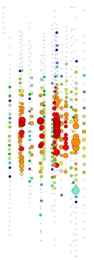
47 Figure 3.4: A muon event in the AMANDA detector. As the muon passes through the detector, light is emitted at a constant rate. 27

48 28

49 29 will produce a second hadronic cascade. This cascade is very difficult to resolve from the first, making it indistinguishable from a cascade produced by an electron, except at very high energies where the tau may travel hundreds of meters. For events that are contained within the detector, this double bang topology is a very distinctive signature, as seen in Fig Muon Energy Loss Cherenkov Radiation A charged particle moving through a transparent medium with refractive index n > 1 with speed v > c/n will produce Cherenkov radiation. Cherenkov radiation is emitted at an angle of cos θ C = 1 βn. (3.7) For energies relevant to AMANDA, β 1. The refractive index of ice is n = Substituting these values into equation 3.7 yields Θ c = 41. (3.8) The energy loss due to Cherenkov radiation is 10 3 MeV/cm, relatively small compared to the total ionization loss of approximately 2 MeV/cm for minimally ionizing particles [35]. Nonetheless, a muon emits 200 photons/cm, which is enough for detection [36].

50 Figure 3.6: A tau event in the future IceCube detector. The two cascades of light are produced by the initial neutrino-nucleon interaction and subsequent decay of the tau particle. 30

51 Stochastic Energy Deposition Muons can lose energy through several mechanisms: ionization, bremsstrahlung, pair production, and photo-nuclear processes. Ionization is a quasi-continuous process and can be treated continuously, while the others are stochastic in nature. The average rate of stochastic energy loss is nearly proportional to the muon energy. The total rate of energy loss of a muon traveling through ice per unit length can be parameterized by de µ dx = a(e µ) + b(eµ) E µ (3.9) where a is the energy loss due to ionization and b E is the energy loss due to stochastic processes [34]. In ice the value of a is approximately 0.2 GeV/m [34] and value of b is approximately m 1. Thus, stochastic events are the main component of energy loss for muons above 600 GeV.

52 32 Chapter 4 The AMANDA Detector AMANDA (the Antarctic Muon and Neutrino Detector Array) is an ice Cherenkov telescope located beneath the ice at the Amundsen-Scott South Pole Station. The detector is an array of 677 photomultiplier tubes and was built over the course of five years. Its primary mission is the detection of neutrinos originating from astrophysical sources. 4.1 History The first effort to build an under-ice neutrino detector was in the austral summer of 1993/94. Four strings, each with 20 optical modules, were deployed at depths between 800 and 1000 meters. This detector became known as AMANDA- A. Studies of the ice properties at these depths showed the absorption length to be around 200 meters at the peak absorption of the photomultiplier tubes (PMTs) of 400 nm. At the same time, the scattering length was on the order of cm, a value too small to allow the reconstruction of muon trajectories. The scattering length was dominated by tiny air bubbles trapped in the ice. It was thought

53 33 that these bubbles would be absent at 800 m as a result of the phase transition that occurs as the increasing pressure transform the air bubbles into air hydrate crystal. However, due to the low temperatures at the south pole, the diffusion of air molecules into the ice crystalline structure slows down. Thus, the bubbles only completely disappear at about 1300 m [37]. Learning from the experiences with the AMANDA-A array, the 19 strings of AMANDA-II were deployed at greater depths (1500m m) in stages during the austral summers from The Detector The AMANDA detector consists of a three-dimensional array of optical modules (OMs). Each OM consists of an 8 Hamamatsu PMT housed in a glass pressure sphere. The OMs are connected to the surface by an electrical cable which serves two purposes. The cable provides the high voltage necessary to operate the PMT and transmits signals from the PMTs back to the data acquisition (DAQ) system electronics at the surface. As the AMANDA detector grew through years of deployment, the hardware used to construct the detector matured. The first 4 strings of what is now known as the AMANDA detector (then called AMANDA-B4) were deployed in the austral summer of These 86 OMs where connected to the surface by coaxial cable, which provided protection against electronic crosstalk in the cables. Unfortunately, coaxial cable has limitations. Coaxial cable is quite dispersive, resulting

54 34 in distortion during the course of transmission to the surface (10 ns PMT pulses arrive at the surface with a width of more than 400 ns). Coaxial cable is also quite thick, limiting the number of cables that could be bundled together. For these reasons the next 6 strings, which were deployed during the austral summer of , used twisted pair cables. These 6 strings brought the total number of OMs in the array to 302. This new array was named AMANDA-B10. The twisted pair cables had less dispersion (150 ns ns) and allowed more cables per string. However, a great deal of electronic crosstalk was observed in these strings. During the austral summer of another 3 strings were deployed bringing the total number of OMs to 428. These strings had both optical fibers and traditional twisted pair cables. The optical fibers were essentially dispersion free and crosstalk free. However, they were quite fragile and nearly 10% were damaged during the refreeze process. Another change in the deployment of these three strings was that they were to lie at a depth between 1200 m m in order to study the optical properties above and below the detector. The last strings to be added to the array were strings in the austral summer. This marked the completion of the AMANDA-II detector. All OMs on these strings were connected to the surface via optical fibers and traditional twisted pair cables. Some of the modules deployed during this year contained experimental digital technologies under investigation for future ice- Cherenkov detectors. String 18 is comprised entirely of digital optical modules

55 35 Figure 4.1: Top view of the AMANDA-II detector. The radius of the detector is approximately 100 meters. (DOMs). These modules contained analog transient waveform digitizers (ATWDs) which record and digitize the signal in situ and then transmit them to the surface. This technology results in the full retention of waveform information without the need for optical fibers. However, the DAQ electronics are buried with the OMs in the ice, hence, beyond the possibility of repair or upgrade. The complete AMANDA-II detector contains 19 strings, 677 OMs and instruments km 3 of ice. It has a diameter of 200 m and a height of 500 m. The modules on each string are separated by 10 m - 20 m, depending on the string. The strings are arranged in three concentric circles and separated by 30 m - 60 m. Figures 4.1 and 4.2 show the layout of the AMANDA detector.

56 36 Depth surface 50 m snow layer 60 m AMANDA-A 810 m 1000 m 1150 m 200 m 120 m AMANDA-B10 Optical Module 1500 m main cable PMT HV divider pressure housing silicon gel 2000 m light diffuser ball 2350 m AMANDA as of 2000 Eiffel Tower as comparison (true scaling) zoomed in on AMANDA-A (top) AMANDA-B10 (bottom) zoomed in on one optical module (OM) Figure 4.2: Schematic of the geometry of AMANDA-II. AMANDA-A and AMANDA-B10 are shown in expanded view in the center. An optical module is blown up on the right. The Eiffel Tower is shown to illustrate the scale.

57 37 The first strings of the IceCube detector are scheduled to be deployed in the austral summer of The entire IceCube array will contain some 4800 OMs, 80 strings and instrument 1 km 3 of ice. It is scheduled to be completed in All of the OMs in the IceCube array will use the DOM technology. IceCube will be deployed between the depths of 1400 m and 2400 m. 4.3 Data Acquisition The AMANDA detector trigger can come from a variety of sources. In normal mode, the detector is triggered by the detection of photons by a set number of OMs in a preset window of time (majority trigger). For the AMANDA-II year 2000 data set, 24 OMs were required to receive at least 1 photo-electron in a 2.1 µsec time period. The trigger rate was approximately 100 Hz. The data acquisition (DAQ) system, located on the surface, is responsible for reading out event information and storing it to disk. Information read and stored by the DAQ includes the leading edge time (LE) and the width or timeover-threshold (TOT) in the time window 22 µsec before and 10 µsec after the trigger time. The DAQ also records the amplitude of pulses arriving from the OMs. The analog digital converter (ADC) information is recorded during a time window of ±2 µsec around the trigger time. The event time is obtained from a Global Positioning System (GPS) unit. A majority trigger in AMANDA is formed based on hit multiplicity. When an OM detects a photo-electron it sends a pulse to the surface where it is received

58 38 by a Swedish Amplifier (SWAMP) which amplifies the signal. A copy of the signal is then sent to discriminators where the signal is converted to a 2 µsec square pulse. The discriminator sends its output to the Digital Multiplicity Adders (DMAD) where multiple signals are summed and compared to a preset threshold. In 2000, this threshold was set at 24 channels. When the sum crosses the threshold, a stop signal is sent to all time digital converters (TDCs) and a veto of several µsec is sent to the trigger. All channels are then read out and the system reset. 4.4 Ice Properties Understanding the properties of the ice is crucial for the operation of the AMANDA-II detector. Thus, the scattering and absorption properties, which affect the timing and number of photons that reach the OMs, must be throughly understood. Numerous studies using both in-situ light sources and atmospheric muons have been conducted to determine the ice properties. The ice is characterized using three parameters: the scattering length λ b (or the scattering coefficient b = 1/λ b ), the absorption length λ a (or the absorption coefficient a = 1/λ a ), and the average of the cosine of the scattering angle (τ s = cosθ. The effective scattering length is then defined as λ eff b = λ s /(1 τ s ) and its coefficient is b e = 1/λ eff b. The effective scattering and absorption coefficients are shown in Figs. 4.3 and 4.4 as a function of wavelength. Dust grains (about 0.04 microns in size) are the biggest contributors to scattering and absorption in the antarctic ice below 1400 meters. Air bubbles,

59 39 absorption coefficient [m -1 ] / / / / / / /33 λ = 337 nm /50 λ = 370 nm λ = 470 nm / / λ = 532 nm 1/ / depth [m] Figure 4.3: Absorption coefficients as a function of depth at various wavelengths [38]. which were the largest scatterers in the AMANDA-A detector, are squeezed into air hydrate crystals which have nearly the same index of refraction as ice at AMANDA-II depths and pose no problems to light detection. Although the glacial ice in which AMANDA-II is embedded is nearly uniform, climatological events in Earth s past, such as ice ages, have left layers of impurities in the form of dust, soot, etc. These dust layers affect the optical properties of the ice and affect photon propagation. The first measurements of the scattering and absorption coefficients of these layers was done using a YAG laser at a frequency of 532 nm. Figure 4.5 shows the effective scattering coefficient as a function of depth in the detector. The dust

60 40 scattering coefficient [m -1 ] bubbles dominate λ = 337 nm λ = 470 nm λ = 370 nm λ = 532 nm D A B C 1/1 1/ depth [m] 1/50 Figure 4.4: Scattering coefficients as a function of depth at various wavelengths [38]. layers are visible as peaks in the scattering coefficient while the clear layers are visible as valleys.

61 Figure 4.5: Scattering coefficient as a function of depth, indicating the presence of dust layers. On the left side of the plot the depth of the OMs in relation to the dust layers are shown [39]. 41

62 42 Chapter 5 Event Reconstruction and Analysis Tools Reconstruction algorithms in AMANDA, like the hardware used to build it, have developed over time. Reconstructions for both muon tracks and cascades are based on the principle of maximization of a likelihood function. Due to how sparsely the AMANDA detector is instrumented, only a limited set of parameters can be constrained for each event. For muons, these parameters are direction (θ, φ), position(x, y, z), and time (t). 5.1 Direct Walk Reconstruction The direct walk [40, 41, 42] method of reconstruction is a first guess method of reconstruction based on pattern recognition of selected hits from photons that have not scattered much in the ice. First guess methods of reconstruction are very fast analytic algorithms that are used as initial track guesses for more complicated algorithms which will be described in the following sections.

63 The direct walk algorithm looks for track elements which are pairs of hits consistent with a close track such that r 1 r 2 t 1 t 2 c < 30 ns (5.1) where r i is the position of the ith hit and t i is the time of the ith hit. Associated hits, those with small time residuals and appropriate distance from the track element based on time residuals, are selected. Quality criteria such as the number of associated hits, the spread of associated hits, and the hit density along the track element are applied. Track elements that pass these criteria are called track candidates. The final first guess track is then found by searching for clusters in zenith angle of track candidates and calculating the mean of all track candidates belonging to the cluster Maximum Likelihood Reconstruction The maximum likelihood method [42] is a generalization of the χ 2 method. In the limit of Gaussian uncertainties the likelihood, L, is related to χ 2 by 2 ln L = χ 2. These methods attempt to find the track hypothesis that maximizes the likelihood by minimizing logl with respect to the track parameters. In general, the likelihood for a given event E 0, which is a collection of detector responses R i and a hypothesis H j, is written as L (E 0 H j ) = i L i (R i H j ). (5.2) If the hypothesis is true, it then generates the observed pattern of hits. The hypothesis is then allowed to vary and an optimization routine is used to find

64 44 the location H 0 of the global extremum of L. The responses {R i } recorded by AMANDA are the time, t i, and duration, T OT i, of each PMT signal and the peak amplitude, A i, of the largest pulse in each PMT. In the case of muon reconstruction, one assumes that the Cherenkov radiation is generated by a single infinitely long muon track. This is a reasonable assumption for the energies of this analysis which simplifies and speeds up the calculation and optimization. For muons, this reduces the function H to sixdimensions H = H ( x, θ, φ, t) Time Likelihood By applying the assumption of an infinitely long muon track we arrive at the simplified likelihood function. The function depends on the arrival time of the light, L = nhits i=1 p ( t i res d i, η i... ), (5.3) where t i res is the time delay, d i is the distance of the OM from the track, and η i is the orientation of the OM relative to the track. The probability density function of single photons, p (t i res d i, η), was generated by parameterizing Monte Carlo simulations of photon propagation in ice [43]. The negative logarithm of the likelihood function, logl, is then minimized using a Simplex [44] algorithm in an iterative technique, which performs multiple reconstructions of the same event. Each reconstruction starts with a different initial track hypothesis. The results of all iterations are compared to each other.

65 45 The lowest value of logl is taken as the reconstructed track Bayesian Likelihood Bayes theorem allows us to fold in information independent of the measurement into the likelihood function. The theorem states P (A B) P (B) = P (B A) P (A). (5.4) Identifying A with the hypothesis H and B with the hit pattern E and solving for P (H E) gives P (H E) = P (E H) P (H). (5.5) P (E) The quantity P (E H) is the likelihood that the given set of hits would be generated by the hypothesis of interest. P (E) is the probability that a given pattern of hits is observed. This quantity is independent of track parameters and is therefore constant. P (H) is known as the prior and does not depend in any way on the measurement. It is the probability of observing the track and can be calculated prior to the measurement. Thus, P (H E) is the probability of the hypothesis after E is taken into account. Bayesian event reconstruction [45] uses the prior probability function shown in Fig This function is flat over the up-going hemisphere and dependent on zenith angle in the down-going hemisphere. Reconstructing using this technique requires one to maximize the product of the probability density function and the prior. Similar to the time likelihood reconstruction, this is done using the Simplex minimizer and an interactive minimizing technique.

66 Cos(Zenith) Trigger-Level Prior Function Figure 5.1: The prior function used is flat over the up-going hemisphere and dependent on zenith angle in the down-going hemisphere [36].

67 47 Near the horizon the effect of the Bayesian reconstruction is strongest. Since AMANDA-II is narrow, events coming in near the horizon have shorter track lengths, making it difficult to constrain the fit tightly. The prior indicates that tracks from atmospheric muons are more likely than neutrinos. Thus, the reconstruction properly chooses the down-going fit as being more likely. 5.3 Quality Parameters Quality parameters are used for selection criteria during different stages of the analysis. Below are descriptions of the parameters that will be used for this analysis Likelihood Ratio As discussed in the previous section, a Bayesian maximum likelihood fit is performed on the sample to fit muon tracks to the observed events. The functional form used is the negative logarithm of the likelihood. This analysis uses two likelihood ratios, up-to-down and track-to-cascade. The likelihood ratio for upto-down going events is defined as R u/d L = log( L up L down ) (5.6) and the likelihood ratio for track-like to shower-like events is defined as R t/s L = log( L track L shower ). (5.7) L up is the likelihood of the track being up-going and hence from a neutrino and L down is the likelihood of the track being down-going and hence from a cosmic

68 48 ray. L track is the likelihood of the event being from a muon and L shower is the likelihood of the event being from a cascade. The up/down likelihood ratio is the most powerful parameter for separating cosmic ray background events (down-going) from signal neutrinos (up-going) Smoothness Smoothness (S phit ) is a topological parameter that is defined by the distribution of hits along the track. It measures how consistent the observed pattern of hits is with the hypothesis of constant light emission by a muon Number of Direct Hits A direct hit occurs when a photon is delayed little by scattering in the ice between production and detection. This delay is measured relative to the predicted arrival time of an unscattered Cherenkov photon emitted from the appropriate point along the track. Different delay windows exist for counting direct hits. For this analysis a hit is considered direct when it arrives in a window of [-15:75] nanoseconds. Thus, N [ 15:75] dir, is defined as the number of direct hits in an event Track Length The track length is determined by projecting each of the direct hits onto the reconstructed track and measuring the distance between the first and last hits. In this analysis, two different track lengths were defined. The first uses a stricter direct hit definition than described above. For this track length, the direct hits

69 49 are required to arrive in the time window [-15:25] nanoseconds L [15:25] dir (5.8) and the second uses the definition of direct hits from above L [15:75] dir (5.9) where direct hits were required to arrive in the [-15:75] nanosecond window Zenith Angle In this analysis, the zenith angle of the best up-going fit and the zenith angle of the best down-going fit are also used in conjunction with the number of direct hits of the best up-going fit and the number of hits of the best down-going fit to remove coincident muon events from cosmic rays Center of Gravity The center of gravity ( cog) of an event is defined as the mean position of all OMs hit by one or more photons in an event. It is represented mathematically as cog = 1 nch nch r i (5.10) where nch is the number of OMs to receive at least one photon and r i is the distance from the center of the detector to the center of the event. i=0 5.4 The Model Rejection Potential An upper limit on an expected flux can be derived from observation when an experiment fails to detect an expected flux. The method used in this thesis is

70 50 the model rejection potential [47]. It uses the method developed by Feldman and Cousins [46] to find the limit. In the Feldman and Cousins method, the upper limit, µ, is a function of the number of observed events, n o, and the number of predicted background events, n b, µ µ (n o, n b ). (5.11) The flux limit is then calculated by the formula ( ) µcl Φ CL = Φ n s (5.12) where CL is the desired confidence level of the calculation, Φ is the expected flux, and n s is the number of signal events predicted from that flux. Since the actual upper limit cannot be known until looking at the data, simulations can be used to calculate the expected average upper limit. The average upper limit is the sum of the expected upper limits, weighted by their Poisson probability of occurrence. It can be written mathematically as inf n obs µ CL = µ CL (n obs,nb ) (n b) (n n obs )! e n b. (5.13) obs=0 Using the average upper limit, one can find the optimal selection criteria for setting the best limit without using the data. When the optimal selection criteria are applied to the Monte Carlo simulations, they will yield the sensitivity of the experiment. Over an ensemble of identical experiments, the strongest constraint on the expected signal flux will correspond to the set of cuts that minimizes the model rejection factor. The model rejection factor is defined by mrf µ CL n s (5.14)

71 51 where n s is the predicted number of signal events from the expected flux. The model rejection factor can then be used to find the expected upper limit (the sensitivity) defined by ( ) µcl Φ CL = Φ. (5.15) n s The actual experiment is not likely to yield exactly Φ CL. This is because the limit in that case will be based on the observed number of events, which is subject to fluctuations in the background in that particular experiment. The sensitivity, which is the average flux upper limit, would give the average value expected over repeated runs of a real experiment.

72 52 Chapter 6 Data and Monte Carlo Simulations 6.1 Live-Time The total data acquisition time for the year 2000 was days. Taking into account the dead time of the data acquisition system, this corresponds to days of detector live time. During that time there were a total of 1,444,252,130 triggers registered. Of those triggers, 90.7% were formed with the majority trigger, which required at least 24 OMs to have fired during the event. File cleaning was performed to remove problematic files. A problematic file is one that has at least one of the following symptoms N hot > 5 (6.1) N dead > 50 (6.2) N unstable > 10 (6.3) where N hot is the number of OMs with ADC and/or TDC rates greater than 30 Hz, N dead is the number of OMs with ADC and/or TDC rates less than 0.5 Hz,

73 53 Figure 6.1: The optical modules excluded from the 2000 analysis and their status. and N unstable are the number of OMs with unstable ADC and/or TDC rates. The file cleaning removed about four percent of the events and reduced the detector live time to 197 days for the year. 6.2 OM Selection An OM is considered bad if the ADC and/or TDC rate is too high, too low or zero, or if the number of edges from the TDC is too high. Figure 6.1 shows the OMs excluded in In addition to the OMs above, other OMs were excluded on a time-dependent basis in an attempt to increase the effective area of the detector. These OMs demonstrated transient behavior, meaning at certain times of the year the OM operated normally and at others the ADC/TDC rates demonstrated the behavior described above. In order to do this most efficiently, the year was divided into