Inference in Ordered Response Games with Complete Information.

Transcription

1 Inference in Ordered Response Games with Complete Information. Andres Aradillas-Lopez Adam M. Rosen The Institute for Fiscal Studies Department of Economics, UCL cemmap working paper CWP36/14

2 Inference in Ordered Response Games with Complete Information. Andres Aradillas-Lopez Pennsylvania State University Adam M. Rosen UCL and CeMMAP August 29, 2014 Abstract We study econometric models of complete information games with ordered action spaces, such as the number of store fronts operated in a market by a firm, or the daily number of flights on a city-pair offered by an airline. The model generalizes single agent models such as ordered probit and logit to a simultaneous equations model of ordered response, allowing for multiple equilibria and set identification. We characterize identified sets for model parameters under mild shape restrictions on agents payoff functions. We then propose a novel inference method for a parametric version of our model based on a test statistic that embeds conditional moment inequalities implied by equilibrium behavior. Using maximal inequalities for U-processes, we show that an asymptotically valid confidence set is attained by employing an easy to compute fixed critical value, namely the appropriate quantile of a chi-square random variable. We apply our method to study capacity decisions measured as the number of stores operated by Lowe s and Home Depot in geographic markets. We demonstrate how our confidence sets for model parameters can be used to perform inference on other quantities of economic interest, such as the probability that any given outcome is an equilibrium and the propensity with which any particular outcome is selected when it is one of multiple equilibria, and we perform a counterfactual analysis of store configurations under both collusive and monopolistic regimes. Keywords: Discrete games, ordered response, partial identification, conditional moment inequalities. JEL classification: C01, C31, C35. This paper is a revised version of the 2013 CeMMAP working paper CWP33/13. We have benefited from comments from seminar audiences at NYU, Berkeley, UCLA, Cornell, and the June 2013 conference on Recent Contributions to Inference on Game Theoretic Models co-sponsored by CeMMAP and the Breen Family Fund at Northwestern. We thank Eleni Aristodemou, Andrew Chesher, Jeremy Fox, Ariel Pakes, Aureo de Paula, Elie Tamer, and especially Francesca Molinari for helpful discussion and suggestions. Financial support from the UK Economic and Social Research Council through a grant (RES ) to the ESRC Centre for Microdata Methods and Practice (CeMMAP) and through the funding of the Programme Evaluation for Policy Analysis node of the UK National Centre for Research Methods, and from the European Research Council (ERC) grant ERC-2009-StG ROMETA is gratefully acknowledged. Address: Department of Economics, Pennsylvania State University, University Park, PA 16802, United States. aaradill@psu.edu. Address: Department of Economics, University College London, Gower Street, London WC1E 6BT, United Kingdom. adam.rosen@ucl.ac.uk. 1

3 1 Introduction This paper provides set identification and inference results for a model of simultaneous ordered response. These are settings in which multiple economic agents simultaneously choose actions from a discrete ordered action space so as to maximize their payoffs. Agents have complete information regarding each others payoff functions, which depend on both their own and their rivals actions. The agents payoff-maximizing choices are observed by the econometrician, whose goal is to infer their latent payoff functions and the distribution of unobserved heterogeneity. Given the degree of heterogeneity allowed and the dependence of each agent s payoffs on their rivals actions, the model generally admits multiple equilibria. We remain agnostic as to the selection of multiple equilibria, thus rendering the model incomplete, and its parameters set identified. Although our model applies generally to the econometric analysis of complete information games in which players actions are discrete and ordered, our motivation lies in application to models of firm entry. Typically, empirical models of firm entry have either allowed for only binary entry decisions, or have placed restrictions on firm heterogeneity that limit strategic interactions. 1 Yet in many contexts firms may decide not only whether to be in a market, but also how many shops or store fronts to operate. In such settings, the number of stores operated by each firm may reflect important information on firm profitability, and in particular on strategic interactions. Such information could be lost by only modeling whether the firm is present in the market and not additionally how many stores it operates. Consider, for example, a setting in which there are two firms, A and B, with (a, b) denoting the number of stores each operates in a given market. Observations of (a, b) = (1, 3) or (a, b) = (3, 1) are intrinsically different from observations with e.g. (a, b) = (2, 2), the latter possibly reflecting less firm heterogeneity or more fierce competition relative to either of the former. Yet each of these action profiles appear identical when only firm presence is considered, as then they would all be coded as (a, b) = (1, 1). Classical single-agent ordered response models such as the ordered probit and logit have the property that, conditional on covariates, the observed outcome is weakly increasing in an unobservable payoff-shifter. Our model employs shape restrictions on payoff functions, namely diminishing marginal returns in own action and increasing differences in own action and a player-specific unobservable, that deliver an analogous property for each agent. These restrictions facilitate straightforward characterization of regions of unobservable payoff shifters over which observed model outcomes are feasible. This in turn enables the transparent development of a system of conditional moment equalities and inequalities that characterize the identified set of agents payoff functions. When the number of actions and/or players is sufficiently large, the characterization of the identified set can comprise a computationally overwhelming number of moment inequalities. While ideally one would wish to exploit all of these moment restrictions in order to produce the sharpest 1 See e.g. Berry and Reiss (2006) for a detailed overview of complications that arise from and methods for dealing with heterogeneity in such models. 2

4 possible set estimates, this may in some cases be infeasible. We thus also characterize outer sets that embed a subset of the full set of moment inequalities. Although less restrictive, the use of these inequalities can be computationally much easier for estimation and inference. As shown in our application such outer sets can sometimes be used to achieve economically meaningful inference. In our application we apply a parametric version of our model to study capacity decisions (number of stores) in geographic markets by Lowe s and Home Depot. We show that if purestrategy behavior is maintained, a portion of the parameters of interest are point-identified under mild conditions. We provide point estimates for these and then apply a novel inference procedure to construct a confidence set for the entire parameter vector by additionally exploiting conditional moment inequalities implied by the model. 2 In applications primary interest does not always rest on model parameters, but rather quantities of economic interest which can typically be written as (possibly set-valued) functions of these parameters. We illustrate in our application how our model also allows us to perform inference on such quantities, such as the likelihood that particular action profiles are equilibria, and the propensity of the underlying equilibrium selection mechanism to choose any particular outcome among multiple equilibria. This reveals a number of substantive findings within the context of our particular application. We find that when entry by only Lowe s is one of multiple equilibria, there is a much higher propensity for Lowe s to be the sole entrant than there is for Home Depot to be the sole entrant when that outcome is one of multiple equilibria. Additionally we find a greater propensity for the symmetric outcome (1, 1) to obtain when it is one of multiple equilibria than it is for either (0, 1) or (1, 0) to occur when either of those are one of multiple equilibria. Among an array of counterfactual experiments performed under different equilibrium selection rules, we find that those favoring selection of more symmetric outcomes produced features that better match the observed data than do alternative selection rules favoring entry by one firm over the other. We also perform experiments to investigate what market configurations would occur under counterfactual scenarios in which (i) the firms behave cooperatively, and (ii) each firm is a monopolist. Our results indicate that if Lowe s were a monopolist it would operate in many geographic regions where currently only Home Depot is present, while in contrast there are many markets in which only Lowe s is currently present where Home Depot would choose not to open a store. It thus appears that many more markets would go unserved were Home Depot to be a monopolist than if Lowe s were a monopolist. Our method for inference is a criterion function based approach as advocated by Chernozhukov, Hong, and Tamer (2007), which is computationally attractive for the model at hand. Specifically, our criterion function is a quadratic form in the point-identified components of the parameter vec- 2 Other recent papers that feature set identification with a point-identified component but with different approaches include Kaido and White (2014), Kline and Tamer (2013), Romano, Shaikh, and Wolf (2014), and Shi and Shum (2014). The first of these focuses primarily on consistent set estimation, with subsampling suggested for inference. The other three papers provide useful and widely applicable approaches for inference based on unconditional moment inequalities, but do not cover inference based on conditional moment inequalities with continuous conditioning variables, as encountered here. 3

5 tor, which exploits moment equalities implied by the model, and an additional term that captures violations of conditional moment inequalities. Characterization of the asymptotic behavior of the first part is standard. The second component of the quadratic form, denoted ˆR (θ), relies on an unconditional mean-zero restriction implied by the conditional moment inequalities. We show that the asymptotic behavior of this part is determined by a sum of U-processes, and we use results from Hoeffding (1948) and Sherman (1994) to characterize its asymptotic distribution. Because our criterion function is a quadratic form, symmetric around an inverse variance estimator, it is asymptotically distributed chi-square when evaluated at any θ in the region of interest. If none of the conditional moment inequalities are satisfied with equality with positive probability at any such θ, then only the first component of our quadratic form contributes to the asymptotic distribution, which is chi-square with degrees of freedom equal to the dimension of the first component. If, however, any of the conditional moment inequalities are satisfied with equality with positive probability at any θ in the region of interest, then the second component of our quadratic form makes a non-negligible asymptotic contribution, and the degrees of freedom of the limiting chi-square distribution is increased by one. Thus, the use of critical values from this distribution achieves asymptotically valid inference, see Section 5 for details. Inference based on conditional moment inequalities is an active area of research and other possible approaches for estimation and/or inference include those of Andrews and Shi (2013), Chernozhukov, Lee, and Rosen (2013), Lee, Song, and Whang (2013, 2014), Kim (2009), Ponomareva (2010), Armstrong(2011a,b), Chetverikov (2012), and Armstrong and Chan (2013). The paper proceeds as follows. In Section 1.1 we discuss the related literature on simultaneous discrete models, with particular attention to econometric models of games. In Section 2 we define the structure of the underlying complete information game and shape restrictions on payoff functions. In Section 3 we derive observable implications, including characterization of the identified set and computationally simpler outer sets. In Section 4 we provide specialized results for a parametric model of a two player game with strategic substitutes, including point identification of a subset of model parameters. In Section 5 we then introduce our approach for inference on elements of the identified set. In Section 6 we illustrate how our inference method can be applied to behaviorial restrictions other than pure strategy Nash Equilibrium. In particular, we consider behaviorial restrictions that impose rationalizability, and nest Nash Equilibrium in both pure and mixed strategies. In Section 7 we apply our method to model capacity (number of stores) decisions by Lowe s and Home Depot. Section 8 concludes. All proofs are provided in the Appendix. 1.1 Related Literature We consider an econometric model of a discrete game of complete information. Our work follows the strand of literature on empirical models of entry initiated by Bresnahan and Reiss (1990, 1991a), and Berry (1992). Additional early papers on the estimation of complete information discrete games 4

6 include Bjorn and Vuong (1984) and Bresnahan and Reiss (1991b). These models often allow the possibility of multiple or even no equilibria for certain realizations of unobservables, and the related issues of coherency and completeness have been considered in a number of papers, going back at least to Heckman (1978), see Chesher and Rosen (2012) for a thorough review. These issues can be and have been dealt with in a variety of different ways. Berry and Tamer (2007) discuss the difficulties these problems pose for identification in entry models, in particular with heterogeneity in firms payoffs, and Berry and Reiss (2006) survey the various approaches that have been used to estimate such models. The approach we take in this paper, common in the recent literature, is to abstain from imposing further restrictions simply to complete the model. Rather, we work with observable implications that may only set identify the model parameters, a technique fruitfully employed in a variety of contexts, see e.g. Manski (2003), Manski (2007), and Tamer (2010) for references to numerous examples. In the context of entry games with multiple equilibria, this tact was initially proposed by Tamer (2003), who showed how an incomplete simultaneous equations binary choice model implies a system of moment equalities and inequalities that can be used for estimation and inference. Ciliberto and Tamer (2009) apply this approach to an entry model of airline city-pairs, employing inferential methods from Chernozhukov, Hong, and Tamer (2007). Andrews, Berry, and Jia (2004) also consider a bounds approach to the estimation of entry games, based on necessary conditions for equilibrium. Pakes, Porter, Ho, and Ishii (2006) show how empirical models of games in industrial organization can generally lead to moment inequalities, and provide additional inference methods for bounds. Aradillas-López and Tamer (2008) show how weaker restrictions than Nash Equilibrium, in particular rationalizability and finite levels of rationality, can be used to set identify the parameters of discrete games. Beresteanu, Molchanov, and Molinari (2011) use techniques from random set theory to elegantly characterize the identified set of model parameters in a class of models including entry games. Galichon and Henry (2011) use optimal transportation theory to likewise achieve a characterization of the identified set applicable to discrete games. Chesher and Rosen (2012) build on concepts in both of these papers to compare identified sets obtained from alternative approaches to deal with incompleteness and in particular incoherence in simultaneous discrete outcome models. What primarily distinguishes our work from most of the aforementioned papers is the particular focus on a simultaneous discrete model with non-binary, ordered outcomes. Simultaneous binary models are empirically relevant and have also proved an excellent expository tool in this literature. However, as discussed above, the extension to ordered action spaces is important from a practical standpoint. Relevant examples of such outcomes include the number of store fronts a firm operates in a market, or the number of daily flights an airline offers for a particular city-pair. Also related are a recent strand of papers on network economies faced by chain stores when setting their store location profiles, including Jia (2008), Holmes (2011), Ellickson, Houghton, and Timmins (2013), and Nishida (2012). These papers study models that allow for the measurement 5

7 of payoff externalities from store location choices across different markets, which, like most of the aforementioned literature, our model does not incorporate. On the other hand, our model incorporates aspects that these do not, by both not imposing an equilibrium selection rule and by allowing for firm-specific unobserved heterogeneity. 3 Some other recent papers specifically consider alternative models of ordered response with endogeneity. Davis (2006) also considers a simultaneous model with a game-theoretic foundation. He takes an alternative approach, employing enough additional structure on equilibrium selection so as to complete the model and achieve point-identification. Also related is Ishii (2005), who studies ATM networks. She uses a structural model of a multi-stage game that enables estimation of banks revenue functions via GMM. These estimates are then used to estimate bounds for a single parameter that measures the cost of ATMs in equilibrium. Chesher (2010) provides set identification results for a single equation ordered response model with endogenous regressors and instrumental variables. Here we exploit the structure provided by the simultaneous (rather than single equation) model. Aradillas-López (2011) and Aradillas-López and Gandhi (2013) also consider simultaneous models of ordered response. In contrast to this paper, Aradillas-López (2011) focusses on nonparametric estimation of bounds on Nash outcome probabilities, and Aradillas-López and Gandhi (2013) on a model with incomplete information. The parametric structure imposed here allows us to conduct inference on economic quantities of interest and perform counterfactual experiments that are beyond the scope of those papers. 2 The Model Our model consists of J economic agents or players J = {1,..., J} who each simultaneously choose an action Y j from the ordered action space Y j = {0,..., M j }. 4 Each set Y j is discrete but M j can be arbitrarily large, possibly infinite. Y (Y 1,..., Y J ) denotes the action profile of all J players, and for any player j J we adopt the common convention that Y j denotes the vector of actions of j s rivals, Y j (Y 1,..., Y j 1, Y j+1,..., Y J ). As shorthand we sometimes write (Y j, Y j ) to denote an action profile Y with j th component Y j and all other components given by Y j. We use Y Y 1 Y J to denote the space of feasible action profiles, and for any player j, Y j Y 1 Y j 1 Y j+1 Y J to denote the space of feasible rival action profiles. The actions of each agent are observed across a large number n of separate environments, 3 Of the papers in this literature, only Ellickson, Houghton, and Timmins (2013) and Nishida (2012) also allow an ordered but non-binary within-market action space. Nishida (2012), in similar manner to Jia (2008), employs an equilibrium selection rule to circumvent the identification problems posed by multiple equilibria. We explicitly allow for multiple equilibria, without imposing restrictions on equilibrium selection. Ellickson, Houghton, and Timmins (2013) allow for multiple equilibria and partial identification, but employ a very different payoff structure. In particular, they model unobserved heterogeneity in market-level payoffs through a single scalar unobservable shared by all firms. In our model, within each market each firm has its own unobservable. 4 The action labels 0,..., M j are of ordinal but not cardinal significance. 6

8 e.g. markets, networks, or neighborhoods. The payoff of action Y j for each agent j is affected by observable and unobservable payoff shifters X j X j R k j and U j R, respectively, as well as their rivals actions Y j. We assume throughout that (Y, X, U) are realized on a probability space (Ω, F, P), where X denotes the composite vector of observable payoff shifters X j, j J, without repetition of any common components. We use P 0 to denote the corresponding marginal distribution of observables (Y, X), and P U to denote the marginal distribution of unobserved heterogeneity U = (U 1,..., U J ), so that P U (U) denotes the probability that U is realized on the set U. We assume throughout that U is continuously distributed with respect to Lebesgue measure with everywhere positive density on R J. The data comprise a random sample of observations {(y i, x i ) : i = 1,..., n} of (Y, X) distributed P 0. The random sampling assumption guarantees identification of P 0. 5 For each player j J there is a payoff function π j (y, x j, u j ) mapping action profile y Y and payoff shifters (x j, u j ) X j R to payoffs satisfying the following restrictions. Restriction SR (Shape Restrictions): The collection of payoff functions (π 1,..., π J ) belong to a class of payoff functions Π = Π 1 Π J such that for each j J, π j (,, ) : Y X j R R satisfies the following conditions. (i) Payoffs are strictly concave in y j : y j Y j, π j ((y j + 1, y j ), x j, u j ) π j ((y j, y j ), x j, u j ) where by convention π j ( 1, x j, u j ) = π j (M j + 1, x j, u j ) =. < π j ((y j, y j ), x j, u j ) π j ((y j 1, y j ), x j, u j ), (ii) For each (y j, x) Y j X, π j ((y j, y j ), x, u j ) exhibits strictly increasing differences in (y j, u j ), namely that if u j > u j and y j > y j, then π j (( y j, y j ), x, uj ) πj ((y j, y j ), x, u j ) < π j (( y j, y j ), x, u j ) πj ( (yj, y j ), x, u j). Restriction SR(i) imposes that marginal payoffs are decreasing in each player s own action y j. It also implies that, for any fixed rival pure strategy profile y j, agent j s best response correspondence is unique with probability one. Restriction SR(ii) imposes that the payoff function exhibits strictly increasing differences in (y j, u j ). It plays a similar role to the monotonicity of latent utility functions in unobservables in single agent decision problems, implying that the optimal choice of y j is weakly increasing in unobservable u j, as in classical ordered choice models. This restriction aids in our identification analysis by guaranteeing the existence of intervals for u j within which any y j maximizes payoffs for any fixed (y j, x). We focus attention on models where the distribution of unobserved heterogeneity is restricted 5 We impose random sampling for simplicity and expositional ease, but our results can be generalized to less restrictive sampling schemes. For instance our identification results require that P 0 is identified, for which random sampling is a sufficient, but not necessary, condition. 7

9 to be independent of payoff shifters, as is common in the literature. This restriction can be relaxed, see e.g. Kline (2012), though at the cost of weakening the identifying power of the model, or requiring stronger restrictions otherwise. Restriction I (Independence): U and X are stochastically independent, with the distribution of unobserved heterogeneity P U belonging to some class of distributions P U. In our model a structure satisfying Restrictions SR and I is defined as collection of payoff functions (π 1,..., π J ) Π and a distribution of unobserved heterogeneity P U P U. The goal of identification analysis is to deduce which structures (π, P U ) Π P U, and what relevant features of these structures, i.e. functionals of (π, P U ), are admitted by the model and compatible with the distribution of observables P 0. For our identification analysis, the classes Π and P U may each be parametrically, semiparametrically, or nonparametrically specified. If these classes are both parametrically specified, then Π and P U may be indexed by a finite dimensional parameter vector, say θ. Then each θ in some given parameter space Θ represents a unique structure (π, P U ), and identification analysis reduces to deducing which θ Θ have associated structures (π, P U ) that are compatible with P 0. 3 Equilibrium Behavior and Observable Implications In order to close the model and relate structures (π, P U ) to the distribution P 0 of (Y, X), we must additionally specify how players possessing payoff functions π play joint action profiles Y. assume in this paper that players have complete information, and thus know the realizations of all payoff shifters (X, U) when they choose their actions. That is, there is no private information. 6 What then remains is to specify a solution concept for the underlying complete information game. We restrict attention to Pure Strategy Nash Equilibrium (PSNE) as our solution concept to simplify the exposition. Yet our inference approach applies to other solution concepts too (see Section 6 below). This is due to the fact that for inference we exploit observable implications of PSNE that take the form of conditional moment inequalities. We Observable implications of alternative solution concepts, such as rationalizability and (mixed or pure strategy) Nash Equilibrium also give rise to conditional moment inequalities, as shown for example by Aradillas-López and Tamer (2008), Aradillas-López (2011), Galichon and Henry (2011), and Beresteanu, Molchanov, and Molinari (2011), and the inference approach developed in Section 5 can also be readily applied to these alternative systems of conditional moment inequalities. Given our payoff restrictions we wish to emphasize that mixed-strategy Nash Equilibrium behavior can be readily handled through conditional moment inequalities that follow as special cases of the results in Aradillas-López (2011). In Section 6 we describe a behavioral model that nests Nash equilibrium (in either pure or mixed 6 For econometric analysis of incomplete information binary and ordered games see for example Aradillas-López (2010), de Paula and Tang (2012), Aradillas-López and Gandhi (2013) and the references therein. 8

10 strategies) as a special case but allows for incorrect beliefs. There we illustrate how the testable implications compare with those of PSNE and we outline how our inferential approach can be readily applied. A concern in the literature, and a motivation for considering these alternative solution concepts, is the possibility of non-existence of PSNE. However, in games where all actions are strategic complements, or in 2 player games where actions are either strategic substitutes or complements, a PSNE always exists. This follows from observing that in these cases the game is supermodular, or can be transformed into an equivalent representation as a supermodular game. This was shown for the binary outcome game by Molinari and Rosen (2008), based on the reformulation used by Vives (1999, Chapter 2.2.3) for Cournot duopoly. Tarski s Fixed Point Theorem, see e.g. Theorem 2.2 of Vives (1999) or Section 2.5 of Topkis (1998), then implies the existence of at least one PSNE. Our empirical example of Section 7 is a two player game of strategic substitutes, so the existence of PSNE is guaranteed. Nonetheless, in other settings it is possible that no PSNE exists, in which case one could adopt an alternative solution concept and base inference on the resulting conditional moment inequalities. Alternatively, one could consider explicit approaches for dealing with non-existence, or incoherence, as in Chesher and Rosen (2012). For clarity and completeness, we now formalize the restriction to PSNE behavior. To economize on notation, we define each player j s best response correspondence as y j (y j, x j, u j ) arg max π j ((y j, y j ), x j, u j ), (3.1) y j Y j which delivers the set of payoff maximizing alternatives y j for player j as a function of (y j, x j, u j ). Restriction PSNE (Pure Strategy Nash Equilibrium): With probability one, for all j J, Y j = y j (Y j, X j, U j ). Strict concavity of each player j s payoff in her own action under Restriction SR(i) guarantees that y j (y j, X j, U j ) is unique with probability one for any y j, though it does not imply that the equilibrium is unique. It also provides a further simplification of the conditions for PSNE, as summarized in the following Lemma. Lemma 1 Suppose Restriction SR(i) holds. probability one, for all j J, Then Restriction PSNE holds if and only if with π j (Y, X j, U j ) max {π j ((Y j + 1, Y j ), X j, U j ), π j ((Y j 1, Y j ), X j, U j )}, (3.2) where we define π j (( 1, Y j ), X j, U j ) = π j ((M j + 1, Y j ), X j, U j ) =. The proof of Lemma 1 is simple and thus omitted. That Restriction PSNE implies (3.2) is immediate. The other direction follows from noting that if (3.2) holds then violation of (3.1) would 9

11 contradict strict concavity of π j ((y j, Y j ), X j, U j ) in y j. The import of this simple result is a rather large reduction in the number of inequalities required for characterization of PSNE, and hence the identified set of structures (π, P U ). With these restrictions in hand, we now characterize the identified set of structures (π, P U ). Define π j (Y, X, U j ) π j (Y, X j, U j ) π j ((Y j 1, Y j ), X j, U j ), as the incremental payoff of action Y j relative to Y j 1 for any (Y j, X, U j ). From Restriction SR (ii) we have that π j (Y, X, U j ) is strictly increasing in U j and thus invertible. Combining this with Lemma 1 allows us to deduce that for each player j there is for each } (y j, x) an increasing sequence of non-overlapping thresholds, {u j (y j, y j, x) : y j = 0,..., M j+1 with u j (M j+1, y j, x) = u j (0, y j, x) =, such that y j (y j, x j, u j ) = y j u j (y j, y j, x) < u j u j (y j + 1, y j, x). (3.3) That is, given (y j, x), player ( j s best response y j is uniquely ] determined by within which of the non-overlapping intervals u j (y j, y j, x), u j (y j + 1, y j, x) unobservable U j falls. This holds for all j, so under Restriction PSNE each player is best responding to their rivals actions. It follows that with probability one ( U R π (Y, X) u j (Y j, Y j, X), u j (Y j + 1, Y j, X) ]. (3.4) j J In other words, Y is an equilibrium precisely if U belongs to the rectangle R π (Y, X). The notation makes explicit the dependence of the edges of the rectangle on the payoff functions π, through their implied threshold functions u j. We now use this result to characterize the identified set for (π, P U ). Before doing so we further define for any set Ỹ Y and all x X, ) R π (Ỹ, x R π (y, x), y Ỹ which is the union of all rectangles R π (y, x) across y Ỹ, and ) R (x) {U R J : U = R π (Ỹ, x for some Ỹ Y }, to be the collection of all such unions for any x X. 10

12 Theorem 1 Let Restrictions SR, I, and PSNE hold. Then the identified set of structures is S = { (π, P U ) Π P U : U R (x), P U (U) P 0 [R π (Y, X) U X = x] a.e. x X }, (3.5) where, for any x X, R (x) R (x) denotes the collection of sets R (x) U RJ : ) U = R π (Ỹ, x for some Ỹ Y such that nonempty Ỹ1, Ỹ2 Y with ) )) Ỹ 1 Ỹ2 = Ỹ and Ỹ1 Ỹ2 =, P U (R π (Ỹ1, x R π (Ỹ2, x > 0 The above characterization is sharp, and applies under Restrictions SR and I regardless of whether Π and P U are parametrically, semiparametrically, or nonparametrically specfied. That is, the set of pairs (π, P U ) Π P U that satisfy (3.5) all satisfy the restrictions of the model and are compatible with the observed distribution of (Y, X). If there were sufficiently restrictive parameterizations and sufficient variation in exogenous variables for point identification of π and P U, the identified set S would be precisely the singleton set comprising only the identified pair (π, P U ). 7 The characterization (3.5) makes use of results from Chesher and Rosen (2012, 2014) to express the identified set as those (π, P U ) such that the random set R π (Y, X) satisfies the conditional containment functional inequality over the collection of sets U R (x). 8 P U (U) P 0 [R π (Y, X) U X = x], a.e. x X,. (3.6) When Y is finite the identified set coincides with that of other characterizations given in the literature, e.g. Galichon and Henry (2011, Theorem 1) and Beresteanu, Molchanov, and Molinari (2011, Theorem D.2), which incorporate inequalities equivalent to those in (3.5), but over U R (x). The collection R (x) is a sub-collection of coredetermining test sets, as defined by Galichon and Henry (2011, Theorem 1), shown to be sufficient by Chesher and Rosen (2014, Theorem 3) to imply (3.5) for all closed U R J. This characterization comprises fewer conditional moment inequalities while retaining sharpness. Nonetheless, the identified set S expressed in (3.5) may comprise a rather large number of conditional moment inequalities, namely as many as belong to R (x), for each x. More inequality restrictions will in general produce smaller identified sets. Yet the incorporation of a very large 7 For an example of a model satisfying restriction SR and I with point identification under large support conditions, see for example the simultaneous binary model outcome model studied by Tamer (2003). More generally, even parametrically-specified simultaneous equations binary response models allowing for rich forms of unobserved heterogeneity and multiple equilibria yield set rather than point identification, see for example Berry and Tamer (2007) and Ciliberto and Tamer (2009). 8 Note that by definition the collection R (x) contains all sets of the form R π (y, x) for some y Y, since the requirement regarding subsets Ỹ1, Ỹ2 Y holds vacuously when Ỹ = {y}. 11

13 number of inequalities may pose challenges for inference, both with regard to the quality of finite sample approximations as well as computation. As stated in the following Corollary, consideration of those structures satisfying inequality (3.5) applied to only an arbitrary sub-collection of those in R (x), or indeed any arbitrary collection of sets in U, will produce an outer region that contains the identified set. Corollary 1 Let U (x) : X 2 U map from values of x to collections of closed subsets of U. Let S (U) = {(π, P U ) Π P U : U U (x), P U (U) P 0 [R π (Y, X) U X = x] a.e. x X }. Then S S (U). Because S (U) contains the identified set, it can be used to estimate valid, but potentially non-sharp bounds on functionals of (π, P U ), i.e. parameters of interest. Although S (U) is a larger set than S, its reliance on fewer inequalities can lead to significant computational gains for bound estimation and inference relative to the use of S. Even in cases where the researcher wishes to estimate S, it may be faster to first base estimation on S (U). If estimation or inference based on this outer set delivers sufficiently tight set estimates to address the empirical questions at hand, a researcher may be happy to stop here. If it does not, the researcher could potentially refine set estimates or confidence sets based on S (U) by then incorporating additional restrictions, either proceeding to use S (U ) for some superset U of U, or by using S itself. 9 Typically, checking the imposed inequality restrictions involves searching over a multi-dimensional parameter space, so the computational advantage can be substantial. The degree of difference between the size of the outer set S (U) and the identified set may or may not be large. For a given collection of conditional moment inequalities defining S (U), this will depend on the particular distribution of (Y, X) at hand, and is thus an empirical question. In some cases the difference between the outer region and the identified set may be relatively small, while in other cases it may be quite substantial. In the two-player parametric model introduced in the following Section, and used in the application of Section 7, we show that a particular U ( ) is sufficient to point identify all but three of the model parameters, and we are able to achieve useful inferences based on an outer region that makes use of this and other conditional moment restrictions. 9 This will be valid a valid procedure if the researcher can ensure that the confidence sets are constructed such that that one based on the first outer set contains the one based on the second set incorporating further restrictions with probability one. (3.7) 12

14 4 A Two-Player Game of Strategic Substitutes In this section we introduce a parametric specification satisfying Restriction SR for a two-player game with J = {1, 2}. We use this specification in our empirical application, and thus focus particular attention on analysis of this model. We continue to maintain Restrictions I and PSNE. In this model, existence of at least one PSNE a.e. (X,U), is guaranteed by e.g. Theorem 2.2 of Vives (1999) or Section 2.5 of Topkis (1998), as discussed in Section A Parametric Specification For each j J we specify π j (Y, X j, U j ) = Y j (δ + X j β j Y j ηy j + U j ), (4.1) where we impose the restriction that η > 0 to ensure that payoffs are strictly concave in Y j, ensuring Restriction SR(i). Given this functional form, Restriction SR(ii) also holds. In this specification the parameters of the two player s payoff functions differ only in the strategic interaction parameters ( 1, 2 ), though this is not required for our identification analysis. We additionally impose that 1, 2 0, so that actions are strategic substitutes, and existence of PSNE follows as previously discussed. Given this functional form, each player j s best response function takes the form (3.3), namely y j (y j, x j, u j ) = y j u j (y j, y j, x j ) < u j u j (y j + 1, y j, x j ), where for ỹ j = 0, u j (ỹ j, y j, x j ) =, for ỹ j M j + 1, u j (ỹ j, y j, x j ) =, and for all ỹ j {1,..., M j }, u j (ỹ j, y j, x j ) η (2ỹ j 1) + j y j δ x j β. (4.2) In addition we restrict the distribution of bivariate unobserved heterogeneity U to the Farlie- Gumbel-Morgenstern (FGM) copula indexed by parameter λ [ 1, 1]. 10 Specifically U 1 and U 2 each have the logistic marginal CDF and their joint cumulative distribution function is G (u j ) = exp (u j) 1 + exp (u j ), (4.3) F (u 1, u 2 ; λ) = G (u 1 ) G (u 2 ) [1 + λ (1 G (u 1 )) (1 G (u 2 ))]. (4.4) The parameter λ measures the degree of dependence between U 1 and U 2 with correlation coefficient 10 See Farlie (1960), Gumbel (1960), and Morgenstern (1956). 13

15 given by ρ = 3λ/π 2. This copula restricts the correlation to the interval [ 0.304, 0.304]. This is clearly a limitation, but one which appears to be reasonable in our application in Section 7. Note that ρ captures the correlation remaining after controlling for X. Thus with sufficiently many variables included in X a low residual correlation may be reasonable. Naturally, we could use alternative specifications, such as bivariate normal, but the closed form of F (u 1, u 2 ; λ) is easy to work with and provides computational advantages. Compared to settings with a single agent ordered choice model, our framework offers a generalization of the ordered logit model, whereas multivariate normal U generalizes the ordered probit model. For notational convenience we define α η δ and collect parameters into a composite parameter vector θ ( θ 1, θ 2) where θ1 ( α, β, λ ) and θ2 = (η, 1, 2 ). We show in the following Section that under fairly mild conditions the parameter subvector θ 1 is point identified, another advantage of the specification for the distribution of U given in (4.4) Observable Implications of Pure Strategy Nash Equilibrium Given a parametric model, we re-express the sets R π (Y, X) described in (3.4) as R θ (Y, X) in order to indicate explicitly their dependence on the finite-dimensional parameter θ. It follows from (4.2) that observed (Y, X, U) correspond to PSNE if and only if U R θ (Y, X) where R θ (Y, X) { u : η (2Y 1 1) + 1 Y 2 δ X 1 β < u 1 η (2Y 1 + 1) + 1 Y 2 δ X 1 β η (2Y 2 1) + 2 Y 1 δ X 2 β < u 2 η (2Y 2 + 1) + 2 Y 1 δ X 2 β and from Theorem 1 we have the inequality }. (4.5) P U (U) P 0 [R θ (Y, X) U X = x] (4.6) for each U R (x), a.e. x X (see the definition of R (x) in (3.6)). However, it is straightforward to see that Y = (0, 0) is a PSNE if and only if U (, α X 1 β) (, α X 2 β). (4.7) and that when this holds, Y = (0, 0) is the unique PSNE. This follows by the same reasoning as in the simultaneous binary outcome model, see for example Bresnahan and Reiss (1991a) and Tamer (2003), and this observation implies that the conditional moment inequality (4.6) using U = (, α X 1 β) (, α X 2 β) in fact holds with equality Results from Kline (2012) can be used to establish point identification of (α, β) under alternative distributions of unobserved heterogeneity, e.g. multivariate normal, if X is continuously distributed. 12 See also Chesher and Rosen (2012) for general conditions whereby the inequality in (4.6) can be strengthened to equality in simultaneous equations discrete outcome models. 14

16 Specifically, we have from (4.7) with this U that for β ( α, β ), and Zj (1, X j ), P 0 [Y = (0, 0) X = x] = F (Z 1 β, Z2 β; λ ), ) with F (Z 1 β, Z2 β; λ defined in (4.4). Based on this we can construct the partial log-likelihood for the event Y = (0, 0) and its complement as L (b, λ) = n l (b, λ; z i, y i ), (4.8) where l (b, λ; z, y) 1 [y = (0, 0)] log F (z 1 b 1, z 2 b 2 ; λ) + 1 [y (0, 0)] log (1 F (z 1 b 1, z 2 b 2 ; λ)). The following theorem establishes) that under suitable conditions E [L (b, λ)] is uniquely maximized at the population values for ( β, λ, which we denote ( β ), λ. Thus there is point identification of the parameter subset θ 1, which is consistently estimated by the maximizer of (4.8) at the parametric rate. Theorem 2 For each player j {1, 2} let payoffs take the form (4.1), with U X, and let Restriction PSNE hold. Furthermore, assume that (i) for each j {1, 2} there exists no proper linear subspace of the support of Z j (1, X j ) that contains Z j with probability one, and (ii) For all conformable column vectors c 1, c 2 with c 2 0, we have that either P {Z 2 c 2 0 Z 1 c 1 < 0} > 0 or P {Z 2 c 2 0 Z 1 c 1 > 0} > 0. Then: 1. If U has known CDF F, then β is identified. If the CDF of U is only known to belong to some class of distribution functions {F λ : λ Γ}, then the identified set for ( β ), λ takes the form {(b (λ), λ) : λ Γ } for some function b ( ) : Γ B and some Γ Γ. 2. If U has CDF F (, ; λ) given in (4.4) for some λ [ 1, 1], then and uniquely maximizes E [L (b, λ)]. Moreover, ( β, λ ) is point identified n (ˆθ1 θ1) d ( ) N 0, H 1 0, (4.9) where [ l (θ1 ; Z, Y ) l (θ 1 ; Z, Y ) ] H 0 = E. (4.10) θ 1 θ 1 Theorem 2 makes use of two conditions on the variation in X. The first condition is standard, requiring that for each j, Z = (1, X j ) is contained in no proper linear subspace with probably one. This rules out the possibility that X contains a constant component. The second condition 15

17 restricts the joint distribution of Z 1 and Z 2, requiring that conditional on Z j c j < 0 (> 0), Z j c j is nonpositive (nonnegative) with positive probability. This condition is automatically satisfied under well-known semiparametric large support restrictions, for example that X j has a component X jk that, conditional on all other components of X j, has everywhere positive density on R, with β 1k 0. However, it is a less stringent restriction and does not require large support. For example, it immediately applies to the case where Z 1 = Z 2, i.e. with no player-specific payoff shifters, even if all covariates are discrete. The theorem provides a number of useful results. First, there is point identification of the parameters θ 1 if the distribution of unobserved heterogeneity is known. Generally econometric models only restrict the distribution of unobserved heterogeneity to be known (i.e. assumed) to belong to some set of distributions, here P U, indexed by λ Γ with corresponding cumulative distributions F λ. In this case there is, for each fixed distribution, equivalently each λ Γ, a unique β = b (λ) that maximizes the expected log-likelihood when the CDF of unobserved heterogeneity is F λ. Thus, the identified set for θ 1 belongs to the set of pairs (b (λ), λ) such that λ Γ. This can simplify characterization and estimation of the identified set, since for each λ Γ there is only one value of β to consider as a member of the identified set. Thus, for estimation, one need only scan over λ Γ and compute the corresponding maximum likelihood estimator for each such value, rather than search over all values of β B. We further show that when F λ is restricted to the FGM family, there is in fact point identification of λ and hence also of θ 1, which can be consistently estimated via maximum likelihood using the coarsened outcome 1 [Y = (0, 0)]. The parameter vector θ 2 = (η, 1, 2 ) remains in general partially identified. 5 Inference on the Full Parameter Vector To perform inference on θ we combine the results of Theorem 2 above with conditional moment inequalities of the form in Theorem 1 and Corollary 1 over collections of test sets U. These results are summarized by the inequality in (4.6). Our approach will be based on moment functions m k (Y, y, x; θ) consisting of indicators over classes of sets. These sets can be indexed by y, x and θ. Specifically, for moment inequalities of the form given by Theorem 1 and Corollary 1 our moment functions are of the form m k (Y, y, x; θ) = 1 [R θ (Y, x) U k (x, y; θ)] P U (U k (x, y; θ) ; θ), (5.1) where R θ is the rectangle defined in (4.5) and where (y, x) represent given values in Y and X. The first question is how to generate the set of values for (y, x). We use values observed in the data, basing inference on m k (Y, y i, x i ; θ), for i = 1,..., n. To perform inference we employ a statistic 16

18 incorporating density-weighted versions of conditional moment inequalities implied by (4.6). Define T k (y i, x i ; θ) E [m k (Y, y i, x i ; θ) X = x i ] f X (x i ) 0, where m k (Y, y i, x i ; θ) is the moment function defined in (5.1) and where f X ( ) is the density of x. Let (z) + = max {z, 0}. By (4.6) we must have E [ (T k (Y, X; θ)) + ] = 0 for every θ in the identified set. This will be the basis for our inference approach. Our notation U k (x i, y i ; θ) explicitly allows for the test sets U k (x i, y i ; θ), k = 1,..., K, to depend on the observations (y i, x i ) as well as θ. K denotes the number of conditional moment inequalities incorporated for inference (i.e, the collection of classes of sets we use for inference). 13 Given Theorem 1 and Corollary 1 it follows that if the sets U k (x i, y i ; θ), k = 1,..., K, comprise the collection R (x i ) for all i and each θ Θ, then inference is based on the identified set, while for other collections of test sets it is based on an outer set. As discussed in Section 3, the sets R (x i ) may have extremely large cardinality even for moderately large strategy spaces Y, rendering their use impractical. The use of other collections of test sets or moment inequalities implied by the characterization of the identified set given in Theorem 1 may in some cases be computationally advantageous. Consider the function [ K ] R (θ) E (T k (Y, X; θ)) +, k=1 where the expectation is taken with respect to the joint distribution of (Y, X), and ( ) + max {, 0}. The function R (θ) is nonnegative, and positive only for θ that violate the conditional moment inequality E [m k (Y, y i, x i ; θ) X = x i ] 0 for some k = 1,..., K with positive probability. the purpose of inference we employ an estimator for R (θ) that incorporates a kernel estimator, denoted ˆT k (y, x; θ), for T k (Y, X; θ), for each k = 1,..., K. To derive the properties of our estimator we require further regularity conditions, which we now discuss. For the sake of exposition, these conditions are formally stated as Restrictions I1-I6 in Appendix B. We assume throughout that each element of X has either a discrete or absolutely continuous distribution with respect to Lebesgue measure, and we write X = ( X d, X c), where X d denotes the discretely distributed components and X c the continuously distributed components. Convergence rates of conditional expectations estimators therefore depend on z dim (X c ). For kernel-weighting incorporating all components of X we define K (x i x; h) K c ( x c i x c h ) [ 1 x d i = x d], 13 The number of inequalities used can also be allowed to vary with (y i, x i). In this case we could write K (y i, x i) for the number of conditional moment inequalities for (y i, x i) and set m k (Y, y i, x i; θ) = 0 for each i, k with K (y i, x i) < k K max i K (y i, x i). For 17

19 where K c : R z R is an appropriately defined kernel function. The estimators ˆT k (y i, x i ; θ) are then defined as ˆT k (y, x; θ) 1 nh z n m k (y i, y, x; θ) K (x i x; h). (5.2) To establish desirable properties for these estimators we impose in Restriction I1 that the functions f X (x) and T k (y i, x i ; θ) be sufficiently smooth in the continuous components of x. Restriction I2 contains our formal requirements for the kernel function and bandwidth sequences, which are chosen by the researcher. Our approach requires that the bias of each ˆT k (y i, x i ; θ) disappears uniformly at the same rate over the range of values of x i in the data. For this purpose we employ a trimming technique, using only values of conditioning variables x i whose continuous components are contained in the interior of their support. This is done by requiring that x i belongs to a pre-specified set X, such that the projection of X onto X c the continuous components of X is contained in the interior of the projection of X onto X c. In principle we could allow X to depend on n and approach X at an appropriate rate as n. For the sake of brevity, rather than formalize this argument, we presume fixed X and state results for the convergence of ˆR (θ) to an appropriately re-defined R (θ): [ ] K R (θ) E 1 X (T k (Y, X; θ)) +, (5.3) k=1 where 1 Xi 1 [x i Xi ] is our trimming function. In addition, our test statistic replaces the use of the function ( ) + = max {, 0} with the function max {, b n } for an appropriately chosen sequence b n 0. The estimator is thus of the form ˆR (θ) 1 n ( n K [ ] ) 1 Xi ˆT k (y i, x i ; θ) 1 ˆTk (y i, x i ; θ) b n. k=1 The use of the sequence b n allows us to deal with the kink at zero of the function ( ) + while obtaining asymptotically pivotal properties for R(θ). Specific requirements on the choice of b n are given in Restriction I2. Our next restriction, illustrated in Figure 1 and formally stated as Restriction I3, imposes a condition on the behavior of each T k (Y, X; θ). This restriction admits the possibility that P (T k (Y, X; θ) = 0) > 0, i.e. that any of the conditional moment inequalities are satisfied with equality with positive probability. Although inference would be simplified by ruling this out, it is important to allow the possibility of binding inequalities. Our restriction thus allows this, but requires that the density of T k (Y, X; θ) not blow up in a neighborhood to the left of zero. The restriction does allow for T k (Y, X; θ) to have mass points. We next impose with Restriction I4 a condition on the manageability of relevant empirical processes, with manageability as defined in Definition 7.9 of Pollard (1990). Sufficient conditions 18

20 for manageability, which are discussed in the Appendix, comprise restrictions on the classes of functions allowed and are abundant in the empirical process literature. The following Theorem establishes an asymptotically linear representation for ˆR(θ) around R(θ). To do this we employ a Hoeffding projection and results from Sherman (1994). Restriction I5 provides a sufficient condition for application of Sherman s results. It imposes that the kernel of a particular U-process that plays an important role in the derivation of our statistic s asymptotic properties belongs to a Euclidean class. The role of this condition and reference to primitive conditions for it to hold are discussed in Appendix B. Theorem 3 Let Restrictions I1-I5 hold. Then for some a > 1/2, ˆR (θ) = R (θ) + 1 n n ( ψ R (y i, x i ; θ, h n ) + ξ n (θ), where sup ξ n (θ) = O p n a ), θ Θ and where ψ R (y i, x i ; θ, h) = K ( 1Xi (T k (w i, θ)) + E [ ]) 1 Xi (T k (W, θ)) + + [ g (wi ; θ, h) E [ g (W ; θ, h)]]. k=1 We combine the linear representation for ˆR (θ) given by Theorem 3 with the maximum likelihood estimator described in Theorem 2 for θ 1 to perform inference on the set of parameters Θ { θ Θ : } k = 1,..., K, y Y, E [m k (Y, y, X; θ) ) X = x] 0 P 0 [Y = (0, 0) X = x] = F (Z 1 β, Z2 β; λ, a.e. x X. As before, let us group w i (y i, x i ). Let ψ M (w i ) denote the MLE influence function for θ 1. From Theorems 2 and 3 we have that uniformly over θ Θ, for some ɛ > 0, ˆV (θ) n 1/2 (ˆθ1 θ 1 ˆR (θ) ) = n 1/2 ( θ 1 θ 1 R (θ) For inference we use the quadratic form ) ( n 1/2 ) ( ) n + ψ M (w i ) n 1/2 o p (1) n ψ + R (w i ; θ, h n ) o p (n ɛ. (5.4) ) ˆQ n (θ) ˆV (θ) ˆΣ (θ) 1 ˆV (θ), where ˆΣ (θ) (ˆΣMM (θ) ˆΣ MR (θ) ˆΣMR (θ) ˆΣRR (θ) ), 19

21 is an estimator for the variance of ˆV (θ). Specifically, we set ˆΣ MM (θ) ( n 1 n ψ M (w i ) ψ M (w i ) ) 1, ˆΣ MR (θ) n 1 n ψ M (w i ) ˆψ R (w i ; θ, h n ), ˆΣ RR (θ) max { n 1 n ˆψ R (w i ; θ, h n ) 2, κ n }, where ψ M (w i ) and ˆψ R (w i ; θ, h n ) consistently estimate ψ M (w i ) and ψ R (w i ; θ, h n ), respectively, and where κ n 0 is a slowly decreasing sequence of nonnegative constants such that for all ɛ > 0, n ɛ κ n, for example κ n = (log n) 1. This ensures that for any n, ˆΣ RR (θ) is bounded away from zero. In Appendix B we show that using κ n in this way achieves valid inference, as it guarantees that for all θ Θ, Ω 1 (θ) Σ 1 (θ) is positive semidefinite with probability approaching one as n, where ˆΩ (θ) is the same as ˆΣ (θ), but with σ 2 n (θ) = 1 n n ˆψ R (w i ; θ, h n ) 2 in place of ˆΣ RR (θ). Under appropriate regularity conditions, the quadratic form ˆV (θ) is asymptotically distributed χ 2 for any θ Θ, where the degrees of freedom of the asymptotic distribution depend on whether any of the K conditional moment inequalities bind with positive probability P X. If θ Θ and all of the conditional moment inequalities are satisfied strictly at θ, then n 1/2 ˆR (θ) = op (1), and ˆQ n (θ) d χ 2 r, where r dim (θ 1 ). If, on the other hand, θ Θ but at least one of the conditional moment inequalities are satisfied with equality at θ with positive probability, i.e. if θ belongs to the set Θ { θ Θ : P {x X : E [m k (Y, y, X; θ) X = x] = 0} > 0, for at least one k {1,..., K} and some y Y then n 1/2 ˆR (θ) is asymptotically normal and shows up in the asymptotic distribution of ˆQn (θ) such that ˆQ d { n (θ) } χ 2 r+1. Finally, if θ / Θ, then ˆQ n (θ) blows up, i.e. for any c > 0, Pr ˆQn (θ) > c 1 as n. Theorem 4 below uses these results to provide an asymptotically valid confidence set for θ uniformly over θ Θ. The aforementioned distributional results on which it relies are provided in Appendix B. The Theorem requires an additional restriction, namely Restriction I6 in Appendix B, which imposes some mild regularity conditions on the influence function ψ R (w i ; θ, h n ) over θ Θ. We also require that ˆΣ (θ) be within o p (1) of its population counterpart Σ (θ) ( Σ MM (θ) Σ MR (θ) ) Σ MR (θ) Σ, RR (θ) with Σ MM (θ), Σ MR (θ), Σ RR (θ) defined identically to ˆΣ MM (θ), ˆΣ MR (θ), ˆΣ RR (θ), respectively, }, 20

22 but with population expectations E [ ] rather than sample means and taking the limit as h n 0 for Σ MR and Σ RR. Theorem 4 Let Restrictions I1 - I6 hold. Then the set CS 1 α {θ Θ : ˆQ n (θ) c 1 α }, where α > 0, c 1 α is the 1 α quantile of the χ 2 r+1 distribution, and r dim (θ 1) satisfies lim inf P (θ CS 1 α) 1 α, n θ Θ and for all θ / Θ, lim P (θ CS 1 α) = 0. n The confidence set CS 1 α provides correct ( 1 α) asymptotic coverage for fixed P uniformly over θ Θ, and the associated test for θ Θ is consistent against all alternatives θ / Θ. It is worth noting that our CS 1 α can attain good pointwise asymptotic properties, i.e. inf θ Θ lim P (θ CS 1 α) 1 α, n under weaker regularity conditions than those stated here. In particular, with Restrictions I1, I2, I3 maintained we could relax Restrictions I4 and I6, as well as the Euclidean property invoked in Lemma 4, as only sufficient conditions for the asymptotically linear representation of Theorem 3 to hold pointwise in θ would be required. 6 Extensions to More General Behavior Our inferential theory so far has been based on the assumption of Pure Strategy Nash Equilibrium (PSNE) play, but our analysis can be extended to other solution concepts too. To illustrate how this can be done, we now extend our analysis to a more general behavioral model which includes (pure or mixed strategy) Nash Equilibrium as a special case. Let σ j denote player j s subjective beliefs about the probability distribution of Y j. PSNE presupposes these beliefs to be degenerate and correct. Suppose we relax these conditions and assume instead that beliefs satisfy two general conditions: independent randomization and accuracy, which we describe next. Independent randomization (IR): Let σ j denote the true probability distribution of player j s actions. Suppose both players believe that σ 1 σ2 X, U. That is, they believe that players randomize independently given X and U. Note that Nash equilibrium is a special case of this. 21

23 Under condition IR, j s expected utility of choosing Y j = y j is of the form σ j (y j ) π j (y j, y j, X j, U j ) π j (y j, X j, U j ), y j Y j as opposed to the more general form y j Y j σ j (y j y j ) π j (y j, y j, X j, U j ), which allows for correlation in randomization. By strict concavity of payoffs (an assumption we maintain), condition IR immediately implies that player j can be optimally indifferent between at most two choices, which must be consecutive. For a given y j Y j let S(y j ) = { r Y j : y j 1 r y j + 1 }. Under condition IR, if y j is an optimal choice for j, then any other optimal choice must belong in S(y j ). Accuracy of beliefs (AB): Each player j chooses σ j to maximize their expected payoffs given their beliefs. Let Supp ( σ ) j denote the support of j s beliefs. We allow beliefs to be incorrect; however, we maintain that (i) they satisfy Supp ( σ ) j S(Y j ), and (ii) σ j assigns positive probability to no more than two rival actions of the form {r, r + 1}. Note that Nash equilibrium (both in mixed and pure strategies) is a special case of AB. This restriction allows beliefs to be wrong, but not in a completely arbitrary way. Condition AB(i) maintains that j s beliefs assign positive probability to at least one choice that could have been rationalized as optimal (along with the observed choice Y j ) by some beliefs of player j consistent with condition IR. Restriction AB(ii) stipulates that players beliefs respect the fact that their rival can be optimally indifferent between at most two actions, which must be consecutive. Under conditions IR and AB, Supp ( σ ) j must be one of the following five sets, {Y j }, {Y j, Y j 1}, {Y j 1, Y j 2}, {Y j, Y j + 1}, {Y j + 1, Y j + 2}. Let s j (y j ) = min { r Y j : y j 2 r y j + 2 } and s j (y j ) = max { r Y j : y j 2 r y j + 2 }. Given the strategic-substitutes nature of the game studied here, it is not hard to show that (Y 1, Y 2 ) is a rationalizable outcome for some beliefs satisfying IR and AB if and only if ( ) ( ) π j Yj 1, s j (Y j ), X j, U j < πj Yj, s j (Y j ), X j, U j and π j (Y j, s j (Y j ), X j, U j ) > π j (Y j + 1, s j (Y j ), X j, U j ), 22

24 for j = 1, 2. Let R θ (Y, X) { U : } η (2Y 1 1) + 1 s 2 (Y 2 ) δ X 1 β < U 1 η (2Y 1 + 1) + 1 s 2 (Y 2 ) δ X 1 β. η (2Y 2 1) + 2 s 1 (Y 1 ) δ X 2 β < U 2 η (2Y 2 + 1) + 2 s 1 (Y 1 ) δ X 2 β (6.1) If we replace PSNE with the sole assumption that players best-respond to some set of beliefs consistent with conditions IR and AB, then (6.1) replaces the set R θ (Y, X) described in (4.5) and the observable implications described in Section 4.2 would be modified accordingly. By replacing PSNE with this) more general model we would no longer have the equality P 0 [Y = (0, 0) X = x] = F (Z 1 β, Z2 β; λ, and our proof of point identification of β would no longer apply. However, one could still conduct inference with the approach described in Section 5 using conditional moment inequalities of the form 6.1 with R θ (Y, X) in place of R π (Y, X) in Theorem 1. It would thus still be possible to perform the type of counterfactual analyses we present in Section 7. Our results would remain valid if PSNE is the true behavioral model but they would also be valid over a wider range of cases including mixed-strategy NE and cases where players have incorrect beliefs, as long as they are compatible with conditions IR and AB. The cost of course would be that confidence sets based on these less restrictive behaviorial assumptions would be larger. 7 An Application to Home Depot and Lowe s We apply our model to the study of the home improvement industry in the United States. According to IBISWorld, this industry has two dominant firms: Home Depot and Lowe s, whose market shares in 2011 were 40.8% and 32.6%, respectively. We label these two players as Player 1: Lowe s, Player 2: Home Depot. We take the outcome of interest y i = (y i1, y i2 ) to be the number of stores operated by each firm in geographic market i. We define a market as a core based statistical area (CBSA) in the contiguous United States. 14 Our sample consists of a cross section of n = 954 markets in April Table 1 summarizes features of the observed distribution of outcomes. Roughly 75 percent of markets have at most 3 stores. However, more than 10 percent of markets in the sample have 9 stores or more. If we focus on markets with asymmetries in the number of stores operated by each firm, Table 1 suggests that Lowe s tends to have more stores than Home Depot in smaller markets and viceversa. Our justification for modeling this as a static game with 14 The Office of Budget and Management defines a CBSA as an area that consists of one or more counties and includes the counties containing the core urban area, as well as any adjacent counties that have a high degree of social and economic integration (as measured by commute to work) with the urban core. Metropolitan CBSAs are those with a population of 50,000 or more. Some metropolitan CBSAs with 2.5 million people or more are split into divisions. We considered all such divisions as individual markets. 23

25 Table 1: Summary of outcomes observed in the data, including average, median, and percentiles for each of Y 1 and Y 2. Y 1 Y 2 Average Median th percentile th percentile th percentile th percentile Total 1,603 1,880 (%Y 1 > Y 2 ) 33% (%Y 1 < Y 2 ) 25% (%Y 1 + Y 2 > 0) 74% (%Y 1 + Y 2 > 0, Y 1 = Y 2 ) 16% player 1: Lowe s, player 2: Home Depot. PSNE as our solution concept is the assumption that the outcome observed is the realization of a long-run equilibrium. 15 Because there is no natural upper bound for the number of stores each firm could open in a market, we allowed ȳ j to be arbitrarily large. We maintained the assumptions of mutual strategic substitutes and pure-strategy Nash equilibrium behavior with the parametrization described in Section Observable Payoff Shifters For each market, the covariates included in X j were: population, total payroll per capita, land area, and distance to the nearest distribution center of player j for j = {1, 2}. The first three of these were obtained from Census data. Our covariates aim to control for basic socioeconomic indicators, geographic size, and transportation costs for each firm 16. Note that X includes 5 covariates, 3 common to each player as well as the player-specific distances to their own distribution centers. All covariates were treated as continuously distributed in our analysis. Table 1 suggests a pattern where Home Depot operates more stores than Lowe s in larger markets. In the data we found that median market size and payroll were 50% and 18% larger, respectively, in markets where Home Depot had more stores than Lowe s relative to markets where 15 The relative maturity of the home improvement industry suggests that the assumption that the market is in a PSNE, commonly used in the empirical entry literature, is relatively well-suited to this application. Although, as is the case in any industry, market structure evolves over time, 82% of markets in our data exhibited no change in store configuration between March 2009 and September Payroll per capita is included both as a measure of income and as an indicator of the overall state of the labor market in each CBSA. We employed alternative economic indicators such as income per household, but they proved to have less explanatory power as determinants of entry in our estimation and inference results. 24

26 the opposite held. Overall, Home Depot opened more stores than Lowe s in markets that were larger and that had higher earnings per capita. Our methodology allows us to investigate whether these types of systematic asymmetries are owed to the structure of the game, the underlying equilibrium selection mechanism, or unobserved heterogeneity. 7.2 Inference on Model Parameters We began by computing partial maximum likelihood estimates for θ 1, corresponding to those of equation (4.9), Theorem 2. These are shown in the first column of Table 2. Given the ordinal nature of our action space, these point estimates indicate that within a each market, all else equal, a population increase of 100,000 has roughly the same effect on per store profit as a $45 increase in payroll per capita, a 12,300 sq mile increase in land area, or a 400 mile decrease in distance to the nearest distribution center. The second column of Table 2 shows the corresponding 95% CI based on these estimates. Figure 2 depicts the estimated partial log-likelihood for each individual parameter in a neighborhood of the corresponding estimate. Comparing their curvatures, we see that the one for ρ was relatively flatter than those of the remaining parameters. This is reflected in the rather wide MLE 95% CI for ρ. The 95% CI for the coefficients on population and land area include only positive values, while the 95% CI for the coefficient on payroll, though mostly positive, contains some small negative values. The MLE 90% CI for this coefficient (not reported) contained only positive values Test sets for the construction of confidence regions We used the approach described in Section 5 to construct confidence regions for θ. We now describe the class of test sets U k (y i, x i ; θ) we used. As before let R θ be as defined in (4.5). Let Y = {(y 1, y 2 ) Y: y 1 2, y 2 2}, S I θ (x i) = { S R 2 : S = R θ (y, x i ) for some y Y }, S II θ (x i) = { S R 2 : S = R θ (y, x i ) R θ (y, x i ) for some y, y Y such that y y }. We have # ( S I θ (x i) ) = 9 and # ( S II θ (x i) ) = 72. For test sets U k (x i, y i ; θ) we use each element of the collections S I θ (x i) and S II θ (x i) as well as the set R θ (y i, x i ). This yields K = 82 tests sets (not necessarily distinct if y i Y ), and moment functions m k (Y, y i, x i ; θ) = 1 (y i (0, 0)) (1 [R θ (y, x) U k (x i, y i ; θ)] P U (U k (x i, y i ; θ); θ)), k = 1,..., K. (7.1) The term 1 (y i (0, 0)) appears because the likelihood for the event Y = (0, 0) is already incorporated through the partial likelihood estimator ˆθ 1, so the inequalities with y = (0, 0) would be redundant. 25

27 The last column in Table 2 provides 95% projection CIs for each parameter using the approach described in Section 5, using statistic ˆV (θ) defined in (5.4). This statistic incorporated both the moment equalities corresponding to likelihood contributions for the events Y = (0, 0) and Y (0, 0) in the partial log-likelihood, as well as moment inequalities implied by the characterization in Theorem 1. Given the action space, the number of inequalities comprising the identified set would be extremely large. In the interest of computational tractability we restricted attention to those sets U k (x i, y i ; θ) described above 17. Our covariate vector X comprised five continuous random variables. We employed a multiplicative kernel K (ψ 1,..., ψ 5 ) = k(ψ 1 )k(ψ 2 ) k(ψ 5 ), where each k( ) was given by k(u) = 10 l=1 c l (1 u 2) 2l 1 { u 30}, with c 1,..., c 10 chosen such that k( ) is a bias-reducing Biweight-type kernel of order 20. This is the same type of kernel used by Aradillas-López, Gandhi, and Quint (2013). Let z dim(x c ) = 5, and denote ɛ z(2z + 1), α h 1 4z ɛ. For each element of X, the bandwidth used was of the form h n = c σ(x) n α h. 18 The order of the kernel and the bandwidth convergence rate were chosen to satisfy Restriction I2. The constant c was set at The bandwidth b n was set to be at our sample size (n = 954). The regularization sequence κ n was set below machine precision. All the results that follow were robust to moderate changes in our tuning parameters. The region X was set to include our entire sample, so there was no trimming used in our results. Our CS was constructed through a grid search that included over 30 million points. The computational simplicity of our approach makes a grid search of this magnitude a feasible task on a personal computer. 17 As indicated previously, in this application the payoff functions π and the distribution of unobserved heterogeneity P U are known functions of parameters θ. We therefore write R θ (Y, X) in place of R π (Y, X) defined in (3.4), and P U ( ; θ) in place of P U ( ). 18 Note that the use of a different bandwidth for each element of X is compatible with our econometric procedure. This particular choice of bandwidth is in fact equivalent to one using the same bandwidth for each component of X, but where each is first re-scaled by its standard deviation. 19 c = 0.25 is approximately equal to the one that minimizes { [ ( ) ] } 2 AMISE = plim E f(x) f(x) dx, if we employ Silverman s rule of thumb, Silverman (1986), using the Normal distribution as the reference distribution. In this case the constant c simplifies to c = 2 ( π 1/2 (M!) 3 R k (2M) (2M)! (k 2 M ) ) 1 2M+1 1 1, where R k k 2 (u)du, k M u M k(u)du. 1 1 Given our choice of kernel, the solution yields c 0.25, the value we used. 26

28 The third column of Table 2 presents the resulting 95% confidence intervals for each component of θ, i.e. projections given by the smallest and largest values of each parameter in our CS. Relative to the MLE CIs shown in column 2, our confidence intervals are shifted slightly and in some cases larger while in other cases smaller. In classical models where there is point identification ML estimators are asymptotically efficient, and hence produce smaller confidence intervals than those based on other estimators. The comparison here however is not so straightforward. The MLE is based only on the observation of whether each player is in or out of the market, and not the ordinal value of the outcome. The statistic we employ incorporates these likelihood equations as moment equalities and additionally some moment inequalities. That is, these inequalities constitute additional information not used in the partial log-likelihood. Furthermore, the CIs in Table 2 are projections onto individual parameter components, including parameter components for which the profile likelihood carries no information such as the interaction coefficients, 1 and 2. For all of these reasons, neither approach is expected to provide tighter CIs than the other. Reassuringly, the CIs for point-identified parameter components using either method are in all cases reasonably close to each other, yielding qualitatively similar interpretations. One and two-dimensional graphical inspections of our CS did not reveal any holes but we are not sure about the robustness of this feature for our CS given its dimension. Population, land area and distance were the only payoff shifters with coefficient estimates statistically significantly different from zero at the 5% level. The 95% CS for the correlation coefficient ρ was again wide and included zero. The payoff-concavity coefficient η was significantly positive and well above the lower bound of our parameter space, indicating decreasing returns to scale for new stores in a market. Figure 3 depicts joint confidence regions for pairs of parameters. Table 2: Estimates and Confidence Intervals for each Parameter MLE MLE Moment- Estimate 95% CI inequalities 95% CI Population (100,000) [0.869, 3.568] [1.757, 3.792] Payroll per capita ($5 USD) [ 0.023, 0.510] [ 0.064, 0.667] Land Area (1,000 sq miles) [0.027, 0.333] [0.051, 0.409] Distance (100 miles) [ 0.929, 0.159] [ 0.988, 0.410] ρ (Corr(U 1, U 2 )) [ 0.304, 0.204] [ 0.265, 0.302] δ η (Intercept minus concavity coefficient) [ 2.084, 0.534] [ 1.961, 0.656] δ (Intercept) N/A N/A [ 0.351, 5.463] η (Concavity coefficient) N/A N/A [1.076, 6.533] 1 (Effect of Home Depot on Lowe s) N/A N/A [0, 2.741] 2 (Effect of Lowe s on Home Depot ) N/A N/A [0.910, 4.078] ( ) Denotes the individual projection from the joint 95% CS obtained as described in Theorem 4. 27

29 Figure 4 depicts the joint CS for the strategic interaction coefficients, 1 and 2. Our grid search for these parameters covered the two-dimensional rectangle [0, 16] [0, 16]. As we can see, our results strongly suggest that the strategic effect of Lowes on Home Depot (measured by 2 is stronger than the effect of Home Depot on Lowes (measured by 1 ). As we can see in the figure, our CS lies almost entirely outside the 45-degree line, with the latter crossing our CS over a very small range. Our results conclusively excluded the point 1 = 2 = 0, so we can reject the assertion that no strategic effect is present. In particular, while our CS includes 1 = 0, it excludes 2 = 0, leading us to reject the assertion that Lowe s decisions have no effect on Home Depot. 20 Finally, Figure 5 depicts joint confidence sets for strategic interaction coefficients and slope parameters in the model. Once again taking the ML point estimate for the coefficient on population as our benchmark, our 95% CIs on the strategic interaction coefficients from Table 2 can be used to bound the relative effect of interactions on profitability. These indicate that, again all else equal and within a given market, the effect of an additional Home Depot store on Lowe s profit per store is bounded above by that of a population decrease of roughly 156,000. Similarly, the effect of an additional Lowe s store on Home Depot s profit per store is the equivalent of a population decrease of anywhere from roughly 24,000 to 232, Analysis of Equilibrium Likelihood, Selection, and Counterfactual Experiments Primary interest may not lie in the value of underlying model parameters, but rather on quantities of economic interest that can typically be expressed as (sometimes set-valued) functionals of these parameters. Equipped with a confidence set for θ, we now construct confidence regions for several such quantities, namely (i) the probability that a given outcome y is an equilibrium, (ii) the probability that a given outcome y is an equilibrium conditional on a realized outcome Y = y and covariates X = x, (iii) the probability that an equilibrium is selected given it is an equilibrium, and (iv) counterfactual conditional outcome probabilities generated by economically meaningful equilibrium selection rules, including those cases where each firm operates as a monopolist, absent competition from its rival Likelihood of Equilibria Let P E (y x) denote the probability that y is an equilibrium outcome given X = x. From Lemma 1 and (3.3) we have P E (y x) = P U (R θ (y, x) ; θ). 20 We also tried variants of our payoff form specification where strategic interaction was allowed to be a function of market characteristics, including population, population density and relative distance. In all cases our results failed to reject that strategic interaction effect is constant for each firm across markets. 28

30 This relation plays a role in addressing the question: given market characteristics x and the outcome y observed in a given market, what is the probability that some other action profile y was simultaneously an equilibrium, but not selected? We define this as P E (y y, x), which, using the rules of conditional probability, is given by P E ( y y, x ) = P E (y, y x) P E (y x) = P U (R θ (y, x) R θ (y, x) ; θ), P U (R θ (y, x) ; θ) when θ = θ 0, where P E (y, y x) denotes the conditional probability that both y and y are equilibria given X = x. This expression is a known function of θ, and we can construct a 95% CI for P E (y y, x) by collecting the corresponding value for each θ CS 0.95, our confidence set for θ. For the sake of illustration, Table 3 presents results using the realized outcome y = (2, 2) and demographics x observed in CBSA (Amarillo, TX), a metropolitan market. Every outcome y excluded from Table 3 had zero probability of co-existing with (2, 2) as a PSNE. Notice that the lower bound in our CI was zero in each case. Overall, 12 different equilibrium outcomes y could have simultaneously been equilibria with the observed y with positive probability. In seven cases, the probability P E (y y, x) could be higher than 95%. If we consider all outcomes included in Table 3 and think of them as possible counterfactual equilibria in this market, we can see that the total number of stores could have ranged between 3 and 7. The actual number of stores observed here (4) was closer to the lower bound. Our results also uncover structural asymmetries at the market level. For instance, while (4, 1) and (5, 1) could have coexisted as Nash equilibria with the observed outcome, our CS rule out (1, 4) and (1, 5) as equilibrium outcomes. We now consider the unconditional probability that any y Y is an equilibrium, denoted P E (y). By the law of iterated expectations we can write P E (y) = E [P E (y Y, X)], where the expectation is taken over Y, X. For θ = θ 0, a consistent estimator for P E (y) is given by ˆP E (y, θ) 1 n n P E (y y i, x i, θ), P E (y y i, x i, θ) P U (R θ (y, x i ) R θ (y i, x i ) ; θ). P U (R θ (y i, x i ) ; θ) Let ˆσ (θ) denote the sample variance of P E (y Y, X, θ), i.e. ˆσ (θ) 1 n n ( P E (y y i, x i, θ) ˆP E (y, θ)) 2. { If θ 0 were known, then by a central limit theorem, the set ˆPE (y, θ 0 ) ± n 1/2 z αˆσ (θ 0 )} with z α Φ 1 (1 α/2) would provide an asymptotic 1 α CI for P E (y). In practice θ 0 is unknown, but we 29

31 can use the union of such sets over θ values in CS 1 α to construct our CI CI (P E (y)) θ CS 1 α { r [0, 1] : ˆP E (y, θ) n 1/2 z αˆσ (θ) r ˆP } E (y, θ) + n 1/2 z αˆσ (θ). (7.2) If it were known (i.e. with probability one) that θ 0 CS 1 α, then CI (P E (y)) would contain P E (y) with at least probability 1 α asymptotically. With θ 0 CS 1 α with probability bounded below by 1 α asymptotically, CI (P E (y)) provides a nominal 1 2α CI by Bonferroni s Inequality. Table 4 presents the 0.90 (α = 0.05) CI for P E (y) for the ten most frequently observed outcomes in the data. Table 3: Outcomes y that could have co-existed as equilibria with the realized outcome (2, 2) in CBSA (Amarillo, TX). y 95% CI for P E (y Y i, X i ) y 95% CI for P E (y Y i, X i ) (0, 4) [0, ] (4, 0) [0, ] (6, 0) [0, ] (3, 0) [0, ] (4, 1) [0, ] (5, 1) [0, ] (0, 3) [0, ] (0, 5) [0, ] (5, 0) [0, ] (7, 0) [0, ] (1, 3) [0, ] (3, 1) [0, ] Table 4: Outcomes y with the largest aggregate probability of being equilibria, P E (y) y 90% CI for P E (y) Observed frequency (α = 0.05) for y (0, 0) [0.2415, ] (1, 0) [0.1973, ] (1, 1) [0.1224, ] (0, 1) [0.1081, ] (2, 1) [0.0398, ] (1, 2) [0.0120, ] (2, 0) [0.0083, ] (3, 1) [0.0078, ] (2, 2) [0.0065, ] (3, 2) [0.0040, ] (2, 3) [0.0038, ] (3, 3) [0.0045, ] Outcomes ordered by observed frequency. 30

32 7.3.2 Propensity of Equilibrium Selection Our model is silent as to how any particular market outcome is selected when there are multiple equilibria. Nonetheless, a confidence set for θ can be used to ascertain some information on various measures regarding the underlying equilibrium selection mechanism M. Consider for example the propensity that a given outcome y is selected when it is an equilibrium, P M (y) P (Y = y). P E (y) In similar manner to the construction of the CI (7.2) for the probability that some outcome y is an equilibrium, we can construct an asymptotic 1 2α CI for P M (y) as CI (P M (y)) θ CS 1 α { r [0, 1] : ˆP M (y; θ) z α ŝ (θ) r ˆP } M (y; θ) + z α ŝ (θ), where now ŝ (θ) consistently estimates the standard deviation of ˆP M (y; θ) P (Y = y) P E (y; θ). Recall that (0, 0) cannot coexist with any other equilibrium and therefore P M (0, 0) = 1. In Table 5 we present a CI for the selection propensity P M (y) for all other outcomes listed in Table 4. In all cases in Table 5 the upper bound of our CIs was 1, so only the lower bounds of our CIs on the selection probabilities are informative. Table 5: Aggregate propensity P M (y) to select y when it is a PSNE. y 90% CI for P M (y) Observed frequency for y (1, 1) [0.8884, 1] (1, 0) [0.6896, 1] (2, 1) [0.6350, 1] (0, 1) [0.3932, 1] (3, 3) [0.5772, 1] (2, 2) [0.4503, 1] (3, 1) [0.2850, 1] (3, 2) [0.2381, 1] (2, 3) [0.2322, 1] (1, 2) [0.1920, 1] (2, 0) [0.0506, 1] Outcomes ranked by the CI lower bound. 31

33 We can also make direct comparisons of the selection propensities P M (y) across particular profiles. Figure 6 makes such comparisons by plotting ˆP M (y; θ) for each θ CS 1 α. As Figure 4 shows, CS 1 α includes parameter values θ for which 1 = 0. For such values, the optimal decision of Lowes does not depend on the actions of Home Depot; by strict concavity of payoffs, this eliminates the possibility of multiple equilibria for any such θ. Consequently for such parameter values the propensity to select equilibria is always equal to one for any outcome (since any outcome that is an equilibrium must be the unique equilibrium). This explains why the upper bound for P M (y) in our CS is always 1 for any y. However, as Figure 6 shows, our results yield nontrivial lower bounds for these propensities and they also allow us to make comparisons across different outcomes to try to understand whether firms have a particular preference towards certain equilibrium outcomes. With the exception of θ yielding selection propensities very close to one for both outcomes considered in each graph, the comparisons in parts (A)-(C) of Figure 6 can be summarized as follows: (A) Equilibria with at most one store by each firm: We compare the propensity of equilibrium selection for the outcomes (0, 1), (1, 0) and (1, 1). Our results yield two findings: (i) Comparing equilibria where only one store is opened, there is a higher selection propensity for Lowe s to have the only store than for Home Depot. (ii) There is a greater selection propensity for the equilibrium in which both firms operate one store than those where only one firm does. (B) Equilibria with a monopolist opening multiple stores: We focus on the outcomes (0, 2), (2, 0), (0, 3) and (3, 0). Our results indicate that the selection propensity is higher for the outcome in which Lowe s operates two stores than those where Home Depot operates two stores. Our findings regarding selection propensities for (0, 3) and (3, 0) were less conclusive. (C) Equilibria where both firms enter with the same number of stores: We focus on the outcomes (1, 1), (2, 2) and (3, 3). Although not illustrated in the figure, the propensity to select symmetric equilibria where both firms are present appeared to be comparably higher than the propensity to select equilibria where there is only one firm in the market. For most θ CS 1 α, the outcome (1, 1) was the most favored. Without a structural model, the observed frequencies alone are not informative about selection propensities. For example, even though (1, 1) was observed in only 12.5% of markets while (1, 0) was observed in 20.2% of them, our results show that, except for some θ CS 1 α with both selection propensities close to one, the selection propensity for (1, 1) when it was an equilibrium was higher than that of (1, 0). The fact that the latter is observed more frequently simply seems to indicate that payoff realizations where (1, 1) is an equilibrium occurred relatively rarely. 32

34 7.3.3 Counterfactual equilibrium selection rules As explained above, our framework allows us to study the likelihood that other outcomes could have co-existed as equilibria along with the outcomes actually observed in each market in the data. With this information at hand we can do counterfactual analysis based on pre-specified (by us) equilibrium selection mechanisms. Here we generate counterfactual outcomes in each market based on four hypothetical equilibrium selection rules. We focus our analysis on those markets where at least one firm entered and each firm opened at most 15 stores. 21 This accounts for approximately 70% of the entire sample. (A) Selection rule favoring Lowe s. For each market i, a counterfactual outcome y c i (yc i1, yc i2 ) was generated through the following steps: 1. Find all the outcomes y for which { PE (y, Y i, X i θ) P E (y Y i, X i ) = max P E (Y i, X i θ) : θ CS 1 α } (the upper bound within our CS for the probability of co-existing with Y i as NE) was at least 95%. If there are no such outcomes, then set y c i = Y i. Otherwise proceed to step Choose the outcome y with the largest number of Lowe s stores. If there are ties, choose the one with the largest number of Home Depot stores. (B) Selection rule favoring Home Depot. Same as (A), but switching the roles of Home Depot and Lowe s. (C) Selection rule favoring entry by both firms and largest total number of stores. Here we took the following steps to determine y c i : 1. As in (A) and (B), look for all the outcomes y for which P E (y Y i, X i ) If no such y Y i exists, set y c i = Y i. Do the same if no y was found where both firms enter. Otherwise proceed to step Among the outcomes y found in step 1, look for the one that maximizes the total number of stores y 1 + y 2. If there are ties, then choose the one that minimizes y 1 y 2. If more than one such outcome exists, choose randomly among them using uniform probabilities. (D) Selection rule favoring symmetry. Each y c i was generated as follows: 1. As in (A)-(C), look for all the outcomes y for which P E (y Y i, X i ) If no such y Y i exists, set y c i = Y i. Otherwise proceed to step Recall again that observing (0, 0) in a given market implies that no other counterfactual equilibrium was possible. 33

35 2. Among the outcomes y found in step 1, look for the one that minimizes y 1 y 2. If more than one such outcomes exist, choose randomly among them using uniform probabilities. Table 6: Results of counterfactual equilibrium selection experiments Selection rules Observed data (A) (B) (C) (D) Y 1 Y 2 y1 c y2 c y1 c y2 c y1 c y2 c y1 c y2 c Average Median th percentile th percentile th percentile Total 1,180 1,090 3, ,062 2, ,172 1,120 % (y 1 > y 2 ) 47% 64% 17% 44% 33% % (y 1 = y 2 ) 23% 21% 28% 42% 48% ( ) The markets considered in this experiment where those where at least one firm entered and each firm opened at most 15 stores. This included approx. 70% of the entire sample. Examining Table 6, the pattern of market outcomes that results from counterfactual selection rules (A), (B) and (C) is decisively different from the features of the observed outcomes in the data. This is less so for selection rule (D). Table 6 also suggests that a selection mechanism which maximizes the total number of stores in each market (rule (C)) would produce a pattern of outcomes heavily biased in favor of Lowe s. Overall, among these counterfactual experiments, the one employing selection rule (D) favoring symmetry most closely matches the observed pattern of store profiles in the data Counterfactual experiments: cooperation and jointly efficient behavior Our results allow us to analyze counterfactual alternatives to noncooperative behavior. Here, we consider a cooperative counterfactual scenario in which the firms maximize the sum of their payoff functions, assigning equal weight to each. Note that due to the ordinal nature of our game, payoff functions are not measurable in dollars. Nonetheless, maximization of the sum of firm payoffs produces a Pareto efficient outcome. We refer to this behavior as jointly efficient, keeping in mind that it does not incorporate consumer welfare, and that it is not necessarily the unique Pareto efficient counterfactual scenario. Fix a parameter value θ and focus on market i. Let (y i, x i, u i ) denote the realizations of (Y, X, U) in that market. Let (y e 1 (x i, u i ; θ), y e 2 (x i, u i ; θ)) be an element of arg max (y 1,y 2 ) [ ] π 1 (y 1, y 2, x 1,i, u 1,i ; θ) + π 2 (y 1, y 2, x 2,i, u 2,i ; θ), 34

36 so that (y e 1 (x i, u i ; θ), y e 2 (x i, u i ; θ)) denotes an action profile maximizing the sum of firm payoffs. Recall from above that P U (R θ (y, x); θ) denotes the probability that y is an equilibrium outcome given X = x. We are interested in the following two functionals, y e j(y i, x i, θ) = P e (y i, x i, θ) = u R θ (y i,x i ) u R θ (y i,x i ) y e j (x i, u; θ) f (u; λ) du P U (R θ (y i, x i ); θ) for j = 1, 2. [ ] 1 (y 1,i, y 2,i ) = (y1 e (x i, u; θ), y2 e (x i, u; θ)) f(u; λ)du. P U (R θ (y i, x i ); θ) Conditional on X = x i and conditional on y i being an equilibrium outcome, y e j (y i, x i, θ) is the expected jointly efficient choice for j and P e (y i, x i, θ) is the probability that the outcome observed in the i th market is jointly efficient. Using our results, confidence sets for these objects can be constructed as CS ( y e j(y i, x i ) ) = CS (P e (y i, x i )) = θ CS 1 α { r R+ : r = y e j(y i, x i, θ) }, θ CS 1 α {r [0, 1]: r = P e (y i, x i, θ)} We apply this analysis to the 308 (out of 954) markets that had a single store in our sample. We use S 1 to denote this collection of markets. Our goal is to compare observed market outcomes to those that would be obtained under jointly efficient behavior, and in particular to determine whether cooperation would lead to more stores in the markets in S 1. Let T 1 = T 1 = [ ] min y e 1(y i, x i, θ) + y e 2(y i, x i, θ), θ CS 1 α i S 1 max θ CS 1 α i S 1 [ y e 1(y i, x i, θ) + y e 2(y i, x i, θ) [ T 1, T 1 ] is a CI for the total number of stores we would observe in the markets in S1 under a cooperative regime. Of particular interest to us is how 308 (the actual number of stores observed in S 1 ) compares to this CI. Our results yielded [ T 1, T 1 ] = [ 308, ]. ]. Note first that the number of stores observed in these markets corresponds to the lower bound we would observe under cooperation. This is by construction, since the number of stores in markets in S 1 could only be lower if the outcome were (0, 0), which would necessarily produce lower total payoff (specifically zero) than the observed single-entrant PSNE outcome, as otherwise it would not have been a PSNE. On the other hand, a market in which equilibrium resulted in a single entrant could have resulted in more stores under joint efficiency if the firm that did not enter would find it more profitable to operate multiple stores absent the presence of the firm that actually entered. Our counterfactual analysis reveals that we could have as many as 45% more expected stores if firms maximized their 35

37 joint payoffs. Table 7 summarizes some of the main findings of this counterfactual experiment. Table 7: Summary of counterfactual results under cooperation. There exist at least 96 markets (out of 308) where Home Depot had more stores (and Lowe s had fewer stores) than the expected outcome under cooperation. The number of such markets could be as large as 110. There existed parameter values in our confidence set for which every market in S 1 had fewer total stores than under cooperation. The expected number of total stores under cooperation would increase from 1 to at least 2 in as many as 85 markets. There were 286 markets for which we could not reject that P e (y i, x i ) < 50%, 93 markets for which we could not reject that P e (y i, x i ) < 10% and 47 markets for which we could not reject that P e (y i, x i ) < 5%. There were 15 markets for which we could not reject that P e (y i, x i ) = 0. Our results suggest that in this market segment noncooperative behavior has led to less entry by Lowe s and greater entry by Home Depot than would be optimal under the counterfactual cooperative regime. These results are in line with some of the findings in Section which showed a higher propensity to select equilibria favoring Lowe s in markets with at most one store Counterfactual experiment: Monopolistic behavior Our results also allow us to analyze the implications of how each of these firms would behave if their opponent left the industry. For firm j in the i th market let y m j (x j,i, u j,i ; θ) = arg max y j π j ((y j, 0), x j,i, u j,i ; θ) denote the optimal choice if j is the monopolist in market i. Let y m j (y i, x i, θ) = u j R θ (y i,x i ) y m j (x j,i, u j ; θ) f j (u j ) du j P U (R θ (y i, x i ); θ) denote the expected monopolistic choice firm j would make in market i given that the observed outcome there is a PSNE. A CS for this expected choice can be constructed as CS ( y m j (y i, x i ) ) = { r R+ : r = y m j (y i, x i, θ) }. θ CS 1 α 36

38 ( ) We constructed CS y m j (y i, x i ) for every market in our sample. Our main finding is that there is a stark contrast in the monopolistic behavior of both firms. While Lowe s would enter many markets where it has no current presence if Home Depot dropped out of the industry, the opposite is not true: Home Depot would concentrate its presence in relatively fewer markets, remaining out of multiple markets where it currently has no presence. Lowe s on the other hand would spread its presence over a larger geographic area including smaller markets. This can be explained by the geographic distribution of both firms regional distribution centers. Table 8 summarizes some of our main findings. Table 8: Summary of counterfactual results under monopolistic behavior. There exist at least 119 markets where Lowe s is currently absent where it would enter if it were a monopolist. We could not reject that Home Depot would not enter any market where it is currently absent if it were a monopolist. In our data there were 251 markets with no stores. If Lowe s were a monopolist, this number would increase to no more than 257. In contrast, if Home Depot were a monopolist this number could grow to as many as 465 markets (almost half of the total markets in our data). There exist 3,483 stores in our data. If Lowe s were a monopolist the expected number of stores would be at least 2,130. If Home Depot were a monopolist, this number could fall as low as 1,860, constituting approximately a 50% drop). In summary, a sizable number of markets that are currently served by Lowe s (as many as 214) could go unserved by Home Depot if the latter were a monopolist. In contrast, Lowe s would enter almost every market where Home Depot has a presence, staying out of at most 6 such markets. 8 Conclusion In this paper we have analyzed a simultaneous equations model for a complete information game in which agents actions are ordered. This generalized the well-known simultaneous binary outcome model used for models of firm entry to cases where firms take ordered rather than binary actions, for example the number of store fronts to operate in a market, or the number of daily routes offered on a city pair by an airline. We applied recently-developed methods from the literature to characterize (sharp) identified sets for model structures via conditional moment inequalities under easily interpreted shape restrictions. While one may ideally wish to incorporate all of the identifying information delivered by the model 37

39 in performing estimation and inference, the number of implied conditional moment inequalities can be rather large, potentially posing significant challenges for both computation and the quality of asymptotic approximations in finite samples. However, the structure of this characterization lends itself readily to outer regions for model parameters, also characterized by conditional moment inequalities, which may be easier to use for estimation and inference. We further showed that in a parametric two player instance of our model, we achieve point identification of all but 3 parameters under fairly mild conditions, without using large support restrictions. We proposed a novel method for inference based on a test statistic that employed densityweighted kernel estimators of conditional moments, summing over measured deviations of conditional moment inequalities. We used results from the behavior of U-processes to show that our test statistic behaves asymptotically as a chi-square random variable when evaluated at points in the identified set, with degrees of freedom dependent upon whether the conditional moments are binding with positive probability. This was then used to construct confidence sets for parameters, where the critical value employed is simply a quantile of a chi-square distribution with the appropriate degrees of freedom. We applied our inference approach to data on the number of stores operated by Lowe s and Home Depot in different markets. We presented confidence sets for model parameters, and showed how these confidence sets could in turn be used to construct confidence intervals for other quantities of economic interest, such as equilibrium selection probabilities and the probability that counterfactual outcomes are equilibria jointly with observed outcomes in a given market. Our framework and results also allowed us to conduct counterfactual analysis which included collusion as well as monopolistic behavior. Our inference approach can be applied much more generally to models that comprise conditional moment inequalities, with or without identification of a subvector of parameters. Although we focused on Pure Strategy Nash Equilibrium as a solution concept, this was not essential to our inference method. It could alternatively be based on conditional moment inequalities implied by (mixed or pure strategy) Nash Equilibrium, or other solution concepts, such as rationalizability. To illustrate this, we described the testable implications of a behavioral model that nests Nash equilibrium as a special case but allows for incorrect beliefs. Moreover, in our application we only employed a small subset of the conditional moment inequalities comprising the (sharp) identified set. In principle our approach can be applied to sharp characterizations too, but the number of inequalities these incorporate can be rather large. The shear number of conditional moment inequalities raises interesting questions regarding computational feasibility and the accuracy of asymptotic approximations in finite samples, both for our inference approach and others in the literature. Indeed, these issues may arise when considering a large number of unconditional moment inequalities, as considered in important recent work by Menzel (2011) and Chernozhukov, Chetverikov, and Kato (2013). Future research on these issues 38

40 in models comprising conditional moment inequalities with continuous conditioning variables thus seems warranted. References Andrews, D. W. K., S. T. Berry, and P. Jia (2004): Confidence Regions for Parameters in Discrete Games with Multiple Equilibria, with an Application to Discount Chain Store Location, working paper, Yale University. Andrews, D. W. K., and X. Shi (2013): Inference for Parameters Defined by Conditional Moment Inequalities, Econometrica, 81(2), Aradillas-López, A. (2010): Semiparametric Estimation of a Simultaneous Game with Incomplete Information, Journal of Econometrics, 157(2), (2011): Nonparametric probability bounds for Nash equilibrium actions in a simultaneous discrete game, Quantitative Economics, 2, Aradillas-López, A., and A. Gandhi (2013): Robust Inference of Strategic Interactions in Static Games, working paper, University of Wisconsin. Aradillas-López, A., A. Gandhi, and D. Quint (2013): Identification and Inference in Ascending Auctions with Correlated Private Values, Econometrica, 81, Aradillas-López, A., and E. Tamer (2008): The Identification Power of Equilibrium in Simple Games, Journal of Business and Economic Statistics, 26(3), Armstrong, T. B. (2011a): Asymptotically Exact Inference in Conditional Moment Inequality Models, Working paper. Yale University. (2011b): Weighted KS Statistics for Inference on Conditional Moment Inequalities, Working paper. Stanford University. Armstrong, T. B., and H. P. Chan (2013): Multiscale Adaptive Inference on Conditional Moment Inequalities, Discussion Paper 1885, Cowles Foundation. Asparouhova, E., R. Golanski, K. Kasprzyk, R. Sherman, and T. Asparouhov (2002): Rank Estimators for a Transformation Model, Econometric Theory, 18, Beresteanu, A., I. Molchanov, and F. Molinari (2011): Sharp Identification Regions in Models with Convex Moment Predictions, Econometrica, 79(6),

41 Berry, S. (1992): Estimation of a Model of Entry in the Airline Industry, Econometrica, 60(4), Berry, S., and P. Reiss (2006): Empirical Models of Entry and Market Structure, in The Handbook of Industrial Organization, ed. by M. Armstrong, and P. Rob, vol. 3, pp North-Holland. Berry, S., and E. Tamer (2007): Identification in Models of Oligopoly Entry, in Advances in Economics and Econometrics: Theory and Applications, Ninth World Congress, Volume II, ed. by R. Blundell, W. Newey, and T. Persson, pp Cambridge University Press. Bjorn, P., and Q. Vuong (1984): Simultaneous Equations Models for Dummy Endogenous Variables: A Game Theoretic Formulation with an Application to Labor Force Participation, CIT working paper, SSWP 537. Bresnahan, T. F., and P. J. Reiss (1990): Entry in Monopoly Markets, Review of Economic Studies, 57, (1991a): Empirical Models of Discrete Games, Journal of Econometrics, 48(1-2), (1991b): Entry and Competition in Concetrated Markets, Journal of Political Economy, 99(5), Chernozhukov, V., D. Chetverikov, and K. Kato (2013): Testing Many Moment Inequalities, CeMMAP working paper CWP65/13. Chernozhukov, V., H. Hong, and E. Tamer (2007): Estimation and Confidence Regions for Parameter Sets in Econometric Models, Econometrica, 75(5), Chernozhukov, V., S. Lee, and A. Rosen (2013): Inference, Econometrica, 81(2), Intersection Bounds, Estimation and Chesher, A. (2010): Instrumental Variable Models for Discrete Outcomes, Econometrica, 78(2), Chesher, A., and A. Rosen (2012): Simultaneous Equations Models for Discrete Outcomes: Coherence, Completeness, and Identification, CeMMAP working paper CWP21/12. (2014): Generalized Instrumental Variable Models, CeMMAP working paper CWP04/14. Chetverikov, D. (2012): Adaptive Test of Conditional Moment Inequalities, Working paper. MIT. 40

42 Ciliberto, F., and E. Tamer (2009): Market Structure and Multiple Equilibria in Airline Markets, Econometrica, 77(6), Davis, P. (2006): Estimation of Quantity Games in the Presence of Indivisibilities and Heterogeneous Firms, Journal of Econometrics, 134, de Paula, A., and X. Tang (2012): Inference of Signs of Interaction Effects in Simultaneous Games with Incomplete Information, Econometrica, 80(1), Ellickson, P. B., S. Houghton, and C. Timmins (2013): Estimating Network Economies in Retail Chains: A Revealed Preference Approach, Rand Journal of Economics, 44(2), Farlie, D. (1960): The Performance of Some Correlation Coefficients for a General Bivariate Distribution, Biometrika, 47, Galichon, A., and M. Henry (2011): Set Identification in Models with Multiple Equilibria, Review of Economic Studies, 78(4), Gumbel, E. (1960): Bivariate Exponential Distributions, Journal of the American Statistical Association, 55, Heckman, J. J. (1978): Dummy Endogenous Variables in a Simultaneous Equation System, Econometrica, 46, Hoeffding, W. (1948): A Class of Statistics with Asymptotically Normal Distribution, Annals of Mathematical Statistics, 19, Holmes, T. J. (2011): The Diffusion of Wal-Mart and Economies of Density, Econometrica, 79(1), Ishii, J. (2005): Interconnection Pricing, Compatibility, and Investment in Network Industries: An Empirical Study of ATM Surcharging in the Retail Banking Industry, working paper, Harvard University. Jia, P. (2008): What Happens When Wal-Mart Comes to Town: An Empirical Analysis of the Discount Retailing Industry, Econometrica, 76, Kaido, H., and H. White (2014): A Two-Stage Procedure for Partially Identified Models, Journal of Econometrics, 182(1), Kim, K.-I. (2009): Set Estimation and Inference with Models Characterized by Conditional Moment Inequalities, Working Paper. University of Minnesota. 41

43 Kline, B. (2012): Identification of Complete Information Games, Working Paper. University of Texas at Austin. Kline, B., and E. Tamer (2013): Default Bayesian Inference in a Class of Partially Identified Models, Working Paper, Northwestern University. Lee, S., K. Song, and Y.-J. Whang (2013): Testing Functional Inequalities, Journal of Econometrics, 172(1), (2014): Testing for a General Class of Functional Inequalities, CeMMAP working paper CWP09/14. Manski, C. F. (2003): Partial Identification of Probability Distributions. Springer-Verlag, New York. MA. (2007): Identification for Prediction and Decision. Harvard University Press, Cambridge, Menzel, K. (2011): Consistent estimation with many moment inequalities, Working Paper. New York University. Molinari, F., and A. M. Rosen (2008): The Identification Power of Equilibrium in Games: The Supermodular Case, a Comment on Aradillas-Lopez and Tamer (2008)., Journal of Business and Economic Statistics, 26(3), Morgenstern, D. (1956): Einfache Beispiele zweidimensionaler Verteilungen, Mathematische Statistik, 8, Nishida, M. (2012): Estimating a Model of Strategic Network Choice, Working Paper, Johns Hopkins University. Nolan, D., and D. Pollard (1987): U-Processes: Rates of Convergence, Annals of Statistics, 15, Pakes, A., and D. Pollard (1989): Simulation and the Asymptotics of Optimization Estimators, Econometrica, 57(5), Pakes, A., J. Porter, K. Ho, and J. Ishii (2006): The Method of Moments with Inequality Constraints, working paper, Harvard University. Pollard, D. (1984): Convergence of Stochastic Processes. Springer Verlag. (1990): Empirical Processes: Theory and Applications. Institute of Mathematical Statistics. 42

44 Ponomareva, M. (2010): Inference in Models Defined by Conditional Moment Inequalities with Continuous Covariates, Working Paper. University of Western Ontario. Romano, J. (2004): On non-parametric testing, the uniform behaviour of the t-test and related problems, Scandinavian Journal of Statistics, 31, Romano, J., A. Shaikh, and M. Wolf (2014): A Practical Two-Step Method for Testing Moment Inequalities, Econometrica, forthcoming. Sherman, R. (1994): Maximal Inequalities for Degenerate U-Processes with Applications to Optimization Estimators, Annals of Statistics, 22, Shi, X., and M. Shum (2014): Simple Two-Stage Inference for a Class of Partially-Identified Models, Econometric Theory, forthcoming. Silverman, B. (1986): Density estimation for statistics and data analysis. Chapman and Hall/CRC. Tamer, E. (2003): Incomplete Simultaneous Discrete Response Model with Multiple Equilibria, Review of Economic Studies, 70(1), (2010): Partial Identification in Economics, Annual Review of Economics, 2, Topkis, D. M. (1998): Supermodularity and Complementarity. Princeton University Press. Vives, X. (1999): Oligopoly Pricing. MIT Press. A Proofs of Results in Sections 3 and 4 In this section we provide proofs for the results of Section 3. Proof of Theorem 1. Let R π (Y, X) be the rectangles described in (3.4). It follows from Theorem 1 of Chesher and Rosen (2012) that the identified set is given by S = { (π, P U ) Π P U : U F ( R J), P U (U) P 0 [R π (Y, X) U X = x] a.e. x X }, (A.1) where F ( R J) denotes all closed sets in R J. This is equivalent to the characterizations of Galichon and Henry (2011, Theorem 1) and Beresteanu, Molchanov, and Molinari (2011, Theorem D.2) applicable with finite Y, specifically { S = (π, P U ) Π P U : C 2 Y, P U ( y C : y PSNE (π, X, U) X = x) P 0 [Y C X = x] a.e. x X }, 43

45 where PSNE (π, X, U) denotes the set of PSNE when the payoff functions are π for the given (X, U). It follows from Chesher and Rosen (2014, Theorem 3) that (A.1) can be refined by replacing F ( R J) with the sub-collection R (x). Proof of Corollary 1. This follows from the observation that for any x X, U R (x), P U (U) P 0 [R π (Y, X) U X = x] (A.2) implies that the same inequality holds for all U R (x), and in particular for all U U (x). Proof of Theorem 2. We prove parts 1 and 2 in the statement of the Theorem in separate steps. Step 1. Suppose that F is known and define the sets S + b {z : z 1 (b 1 β 1) > 0 z 2 (b 2 β 2) 0}, S b {z : z 1 (b 1 β 1) < 0 z 2 (b 2 β 2) 0}. For any z S + b we have that F (z 1 b 1, z 2 b 2 ) > F (z 1 β 1, z 2 β 2) = P {Y = (0, 0) z}, and likewise for any z S b, F (z 1 b 1, z 2 b 2 ) < F (z 1 β 1, z 2 β 2) = P {Y = (0, 0) z}. The probability that Z S b S + b S b is P {Z S b } = P { Z S + } { } b + P Z S b ( P {Z 2 (b 2 β = 2) 0 Z 1 (b 1 β 1) > 0} P {Z 1 (b 1 β 1) > 0} +P {Z 2 (b 2 β 2) 0 Z 1 (b 1 β 1) < 0} P {Z 1 (b 1 β 1) < 0} ). Both P {Z 1 (b 1 β 1) > 0} and P {Z 1 (b 1 β 1) < 0} are strictly positive by (i), and at least one of P {Z 2 (b 2 β 2) 0 Z 1 (b 1 β 1) > 0} and P {Z 2 (b 2 β 2) 0 Z 1 (b 1 β 1) < 0} must be strictly positive by (ii). Therefore P {Z S b } > 0, implying that with λ known b is observationally distinct from β since for each z S b, P {Y = (0, 0) z} F (z 1 b 1, z 2 b 2 ). If instead F is only known to belong to some class of distribution functions {F λ : λ Γ}, the above reasoning implies that for each λ Γ, E [L (b, λ)] is uniquely maximized with respect to b. Then the conclusion of the first claim of the Theorem follows letting b (λ) denote the maximizer of E [L (b, λ)] for any λ Γ. Step 2. Suppose now that U has CDF F (, ; λ) of the form given in (4.4) for some λ [ 1, 1]. 44

46 To show that λ is identified, consider the expectation of the profiled log-likelihood: L 0 (λ) E [L (b (λ), λ)] = E [l (b (λ), λ; Z, Y )]. Note that because ( β ), λ maximizes E [L (b, λ)] with respect to (b, λ), it follows that λ maximizes L 0 (λ) = max b E [L (b, λ)]. That λ is the unique maximizer of L 0 (λ), and thus point-identified, follows from strict concavity of L 0 (λ) in λ, shown in Lemma 2 below. A standard mean value theorem expansion for maximum likelihood estimation then gives ˆθ1 = θ n n ψ M (y i, x i ) + o p (n 1/2), where ψ M (y i, x i ) H0 1 l (θ 1 ; z i, y i ) θ 1 is the maximum likelihood influence function satisfying n 1/2 n ψ M (y i, x i ) N ( 0, H0 1 ), with H 0 as defined in (4.10). Lemma 2 Let the conditions of Theorem 2 hold and assume that U has CDF F (, ; λ ) given in (4.4) for some λ [ 1, 1]. Then L 0 (λ) defined in the proof of Theorem 2 is strictly concave in λ. Proof. conditions: By definition, for any λ [ 1, 1], β (λ) satisfies the first and second order necessary L 0 (β (λ), λ) β = 0, 2 L 0 (β (λ), λ) β β 0, (A.3) where 0 denotes non-positive definiteness. These conditions require, respectively, g (λ, β) E [m 1 (λ, z) df ] = 0, (A.4) β at β = β (λ), and E [m 2 (λ, z) F F β β + m 1 (λ, z) 2 F ] β β 0, (A.5) where for ease of notation p (z) P 0 [Y = (0, 0) Z = z], and for any parameter µ, F µ df (z 1β, z 2 β; λ), evaluated at β = β (λ), dµ m 1 (λ, z) p (z) F (z 1 β (λ), z 2 β (λ) ; λ) 1 (1 p (z)) (1 F (z 1 β (λ), z 2 β (λ) ; λ)) 1, 45

47 m 2 (λ, z) p (z) F (z 1 β (λ), z 2 β (λ) ; λ) 2 (1 p (z)) (1 F (z 1 β (λ), z 2 β (λ) ; λ)) 2 < 0. We now use these conditions to show concavity of L 0 (λ). Using (A.4), equivalently the envelope theorem, we have that L 0 (λ) λ The second derivative with respect to λ is 2 L 0 (λ) λ 2 [ 2 L (β (λ), λ; z) = E λ β [ L (β (λ), λ; z) = E λ β (λ) λ ]. + 2 L (β ] (λ), λ; z) λ 2 We now proceed to solve for each term in (A.6). To solve for β (λ) we apply the implicit function theorem to (A.4), obtaining λ β (λ) λ In addition we have = g 1 g [m β λ = E F F 2 F ] 1 F 2 β β + m 1 β β E [m F 2 β λ + m 1 2 F β λ ]. (A.6) 2 L (β (λ), λ; z) λ β = m 2 F λ F 2 F (z, λ) β + m 1, (A.7) λ β and 2 L (β (λ), λ; z) λ 2 Putting these expressions together in (A.6) gives, = m 2 2 F λ 2 = 0. 2 L 0 (λ) λ 2 = AB 1 A + D, (A.8) where and F A = E [m F 2 F ] F 2 λ β + m 1 λ β, B = E [m F 2 F ] 2 β β + m 1 β β, D = E [ m 2 ( F λ ) 2 ]. By (A.5), B is negative semi-definite so that AB 1 A 0. Then m 2 0 implies that 2 L 0 (λ) λ 2 0, and strictness of the inequality follows from F (, ; λ) (0, 1). Therefore L 0 (λ) is strictly concave in λ and consequently β and λ are point identified. 46

48 B Proofs of Results in Section 5 We begin by formally stating Restriction I1-I6 and establishing some preliminary Lemmas used to prove our Theorems in Section B.1. We then provide proofs in Section B.2. B.1 Regularity Conditions and Lemmas To characterize the asymptotic behavior of n 1/2 ( ˆR (θ) R (θ) ), we first impose some further restrictions. These entail smoothness restrictions, bandwidth restrictions, and conditions that guarantee manageability of relevant empirical processes. We begin with smoothness restrictions. Restriction I1 (Smoothness): As before, let z dim(x c ). For some M 2z + 1, uniformly in (y, x) Supp(Y, X) and θ Θ, f X (x) and T k (y, x; θ) are almost surely M-times continuously differentiable with respect to x c, with bounded derivatives. Our goal is to characterize sufficient conditions for ˆR (θ) to converge to R (θ) at rate n 1/2. To this end we combine these smoothness restrictions with the use of bias-reducing kernels, and we require the bandwidths h n and b n to converge to zero at appropriate rates, as follows. Restriction I2 (Kernels and bandwidths): K c is a bias-reducing kernel of order M with bounded support, exhibits bounded variation, is symmetric around zero, and sup v R z K (v) K <. The positive bandwidth sequences b n and h n satisfy n 1/2 h z nb n, and there exists ɛ > 0, such that h z/2 n b n n ɛ 0, and n 1/2+ɛ b 2 n 0. In addition, M is large enough such that n 1/2+ɛ b M n 0. Suppose our bandwidths satisfy h n n α h and b n n α b. Then Restriction I2 is satisfied if α h and α b are chosen to satisfy α h = 1 4z ɛ h, α b = ɛ b, with 0 < ɛ h 1 4z (2z + 1), 0 < ɛ b < ɛ h. With these bandwidths, the smallest value of M compatible with Restriction I2 is M = 2z + 1. Combined with the smoothness Restriction I1, our bandwidth and kernel restrictions will be used to establish convergence of ˆR (θ) to R (θ) at rate n 1/2, and asymptotically pivotal properties of ˆR (θ) R (θ), appropriately studentized. Our next restriction, discussed in the main text, is below. Restriction I3 (Behavior of T k (Y, X, θ) at zero from below): There exist constants b > 0 and Ā < such that for all positive b < b and each k = 1,..., K, sup θ Θ P ( b T k (Y, X; θ) < 0) bā. We next state Restriction I4 requiring manageability of relevant empirical processes, as defined in Definition 7.9 of Pollard (1990). In the context of our model, unless stated otherwise, m k is as defined in (5.1). 47

49 Restriction I4 (Manageability of Empirical Processes I): For each k = 1,..., K, (i) the process M {m k (Y i, y, x; θ) K (X i x; h) : (y, x, θ) Supp(Y, X) Θ, h > 0, 1 i n} is manageable with respect to the constant envelope K sup v R K c (v; h), and (ii) there exists a c > 0 such that the process I {1 { c T k (Y i, X i ; θ) < 0} : θ Θ, 0 < c < c, 1 i n}, is manageable with respect to the constant envelope 1. Sufficient conditions for manageability are well-established in the empirical process literature. For example, if the kernel function K c is of bounded variation then Lemma 22 in Nolan and Pollard (1987) and Lemmas 2.4 and 2.14 in Pakes and Pollard (1989) imply that the the class of functions {K (x v; h) : v X, h > 0} is Euclidean, as defined in Pakes and Pollard (1989) Definition 2.7, with respect to the constant envelope K. From here, manageability of M follows, for example, if the classes of functions {g (y) = m k (y, y, x; θ) : (y, x, θ) S Y,X Θ} are Euclidean with respect to the constant envelope 1. Sufficient conditions for this property can be found in Nolan and Pollard (1987) and Pakes and Pollard (1989), for example. Likewise, sufficient conditions for manageability of I can be established, for example, if the class of sets Ψ k {(y, x) S Y,X : c T k (y, x; θ) < 0, θ Θ, 0 < c < c} have polynomial discrimination (see Pollard (1984) Definition 13) of degree at most r <. Lemma 1 of Asparouhova, Golanski, Kasprzyk, Sherman, and Asparouhov (2002) provides a sufficient condition for this to hold, namely that the number of points at which T k (y, x; ) changes sign be uniformly bounded over (y, x) S Y,X and k = 1,..., K. The linear representation for ˆR (θ) around R (θ) established in Theorem 3, relies on two parts. First we establish the effect of the use of the threshold b n with respect to ˆT k (Y, X; θ) in ˆR (θ) in place of the zero threshold for T k (y i, x i, θ) in R (θ). We then use a Hoeffding (1948) projection and results from Sherman (1994) to establish the asymptotically linear representation, and the corresponding influence function for characterizing the limiting behavior of n 1/2 ( ˆR (θ) R (θ) ). To establish the first result, define R (θ) 1 n ( n K ) 1 Xi ˆT k (y i, x i ; θ) 1 {T k (y i, x i, θ) 0}, (B.1) k=1 which is equivalent to ˆR { } (θ) but for the replacement of 1 ˆTk (y i, x i ; θ) b n with 1 {T k (y i, x i, θ) 0}. With the following Lemma we establish that R (θ) and ˆR (θ) are uniformly close, specifically that 48

50 they differ by no more that o p ( n 1/2 ) uniformly in θ. Lemma 3 Let Restrictions I1-I4 hold. Then there exists a > 1/2 such that sup R (θ) ˆR ( (θ) = O p n a ). θ Θ With Lemma 3 established, the task of producing a linear representation for n 1/2 ( ˆR (θ) R (θ) ) is simplified to establishing such a representation for n 1/2 ( R (θ) R (θ) ), which does not depend on the bandwidth b n. For notational convenience let us group W (X, Y ). With some minor algebraic manipulation of R (θ) defined in (B.1) and use of the definition of ˆT k (w i ; θ) given in (5.2) we obtain R (θ) = 1 n n K K 1 1 Xi (T k (w i, θ)) + + n 2 k=1 k=1 n l=1 n v k (w l, w i ; θ, h n ), (B.2) where ( ) 1 v k (w l, w i ; θ, h n ) h z m k (y l, y i, x i ; θ) K (x i x l ; h n ) T k (w i, θ) 1 Xi 1 {T k (w i, θ) 0}. (B.3) n In the proof of the following Lemma, we write the second term of (B.2) as a sum of three component terms. We use our smoothness restrictions and a result of Sherman (1994) to establish that all but one of these is uniformly O p (n a ) for some a > 1/2. For application of Sherman s result we further impose the following restriction. Restriction I5 (Euclidean Class): For each k = 1,..., K, the class of functions V k = {v : v (w 1, w 2 ) = v k (w 1, w 2 ; θ, h), θ Θ, h > 0}, is Euclidean with respect to an envelope V such that E [ V 2+δ ] < for some δ > 0. For the definition of Euclidean classes we refer to Definition 2.7 in Pakes and Pollard (1989) or Definition 3 in Sherman (1994). Primitive conditions to establish this property can be found, e.g., in Nolan and Pollard (1987), Pakes and Pollard (1989) and Sherman (1994). In fact, our proof method only requires that the U-process produced by the class V k satisfy the maximal inequality in Sherman (1994), for which the Euclidean property is sufficient. Lemma 4 Let Restrictions I1-I5 hold. Then for some a > 1/2, and for each k = 1,..., K, uniformly 49

51 in θ Θ, 1 n 2 n l=1 n v k (w l, w i ; θ, h n ) = 1 n n ( [ g k (w i ; θ, h n ) E [ g k (W ; θ, h n )]] + O p n a ). where v k (w l, w i ; θ, h n ) is as defined in (B.3) and where g k (w; θ, h) ( v k ( w, w ; θ, h ) + v k ( w, w; θ, h )) df W ( w ). These Lemmas, proven below, are used to prove Theorem 3, which establishes the resulting linear approximation for ˆR (θ). Finally, as discussed in the main text, for the proof of Theorem 4 we require the following addition restriction. Restriction I6 (Regularity on Θ ): Σ MR (θ) and Σ RR (θ) are continuous on Θ and the estimator ˆΣ (θ) is uniformly consistent on Θ, namely sup ˆΣ (θ) Σ n (θ) = o p (1). θ Θ In addition, the following integrability and manageability conditions hold: (i) For some C < and δ > 0, where σ 2 n (θ) var (ψ R (w i ; θ, h n )). lim sup E n θ Θ (ii) The triangular array of processes [ ] ψ R (w i ; θ, h n ) 2+δ C, (θ) σ 2+δ n { ψr (w i ; θ, h n ) : i n, n 1, θ Θ } is manageable with respect to an envelope Ḡ satisfying E [ Ḡ 2] <. B.2 Proofs Proof of Lemma 3. As in the main text, to simplify notation let w (x, y) with support denoted W. We abbreviate ˆT k (w i ; θ) and T k (w i ; θ) for ˆT k (y i, x i ; θ) and T k (y i, x i ; θ), respectively, k = 1,..., K. Suprema with respect to w, θ are to be understood to be taken with respect to W Θ 50

52 unless otherwise stated. Let ξ n (θ) ˆR (θ) R (θ) ( = 1 n K 1 Xi n k=1 ( { } ˆT k (w i ; θ) 1 ˆTk (w i ; θ) b n 1 {T k (w i ; θ) 0}) ). Note that where ξ 1 n (θ) 1 n ξ 2 n (θ) 1 n ξ n (θ) ξ 1 n (θ) + ξ 2 n (θ), ( n K ) 1 Xi ˆT k (w i ; θ) 1 { 2b n T k (w i, θ) < 0}, k=1 ( n K 1 Xi ˆT { } ) k (w i ; θ) 1 ˆTk (w i ; θ) T k (w i, θ) b n. k=1 To complete the proof, we now show that each of these terms is O p (n a ) uniformly over θ Θ for some a > 1/2. Step 1 (Bound on ξ 1 n (θ) ). We have sup ξ 1 n (θ) sup θ θ = + 1 n ( K ) 1 n n 1 Xi T k (w i, θ) 1 { 2b n T k (w i, θ) < 0} ( k=1 n K ) 1 Xi ˆT k (w i, θ) T k (w i, θ) 1 { 2b n T k (w i, θ) < 0} k=1 ( ) ( 2b n + sup ˆT 1 n K k (w i, θ) T k (w i, θ) sup 1 w,θ θ Xi 1 { 2b n T k (w i, θ) < 0}) n k=1 ( )) log n 1 n (2b n + O p sup 1 { 2b nh z n T n k,θ k (w i, θ) < 0} n, (B.4) where the first inequality follows from the triangle inequality, the second from elementary algebra, and the third from sup w,θ ( ) ˆT log n k (w i, θ) T k (w i, θ) = O p nh z n for all k = 1,..., K holding under I2 and I4. Now for b and Ā as defined in Restriction I3 we have 51

53 for all k = 1,..., K and large enough n, 2b n b and therefore sup E [1 { 2b n T k (W, θ) < 0}] 2Āb n, θ Ω n sup V ar [1 { 2b n T k (W, θ) < 0}] 2Āb n. θ (B.5) (B.6) It now follows from the triangle inequality and (B.5) above that for any k = 1,..., K, sup θ 1 n n 1 { 2b n T k (w i, θ) < 0} 1 n sup (1 { 2b n T θ k (w i, θ) < 0} E [ 2b n T k (w i, θ) < 0]) n + 2Āb n. The manageability Restriction I4 implies, using Corollary 4 in Sherman (1994), sup θ 1 n ) n ( Ωn (1 { 2b n T k (w i, θ) < 0} E [ 2b n T k (w i, θ) < 0]) = O p, n which is in fact O p ( b nn ) by virtue of (B.6). Thus sup θ 1 n n 1 { 2b n T k (w i, θ) < 0} ) ( bn = O p + O (b n ) n ( ( ) ) 1 = b n O p + O (1) bn n = b n (o p (1) + O (1)) = O p (b n ). Plugging this into (B.4) we have sup ξ 1 n (θ) = θ ( )) log n (2b n + O p O nh z p (b n ) n ( ) ( ) = O p b 2 b n log n n + Op nh z n = O p ( n a ) for some a > 1/2 by the { bandwidth conditions in Restriction } I2. Step 2 (Bound on P sup w,θ ˆTk (w; θ) T k (w; θ) c ). From Restriction I4 and application of Theorem 3.5 and equation (7.3) of Pollard (1990), there 52

54 exist positive constants κ 1, κ 2 such that for any c > 0, and any U P { sup w,θ } ˆT k (w; θ) T k (w; θ) c ( ( ) ) 2 κ 1 exp nh d nκ 2 c. (B.7) Our smoothness restriction I1 and an M th order expansion imply the existence of a constant C such that Thus sup w,θ { } P sup ˆT k (w; θ) T k (w; θ) b n w,θ [ ] E ˆTk (w; θ) T k (w; θ) Ch M n. { } P sup ˆT [ [ ] k (w; θ, U) E ˆTk (w; θ)] + sup E ˆTk (w; θ, U) T k (w; θ) b n w,θ w,θ { } P ˆT k (w; θ, U) T k (w; θ) b n Ch M n, sup w,θ (B.8) (B.9) where the first inequality follows by the triangle inequality and the second by (B.8). Under our bandwidth restrictions I2 we have for large enough n that b n > Ch M n, and so application of (B.7) to (B.9) with c = b n Ch M n gives { } P ˆT k (w; θ) T k (w; θ) c sup w,θ Step 3 (Bound on ξ 2 n (θ) ). We have ( ( κ 1 exp nh d ( nκ 2 bn Ch M ) ) ) 2 n. (B.10) sup ξ 2 n (θ) sup ˆT { } k (w; θ) sup 1 ˆTk (w; θ) T k (w; θ) b n θ w,θ w,θ { } = O p (1) sup 1 ˆTk (w; θ) T k (w; θ) b n = O p (1) 1 w,θ { sup w,θ } ˆT k (w; θ) T k (w; θ) b n. { Let D n 1 sup w,θ ˆTk (w; θ) T k (w; θ) b n }. Now using Chebyshev s inequality we have ( ) ( ) D n E [D n ] = O p var (Dn ) = O p E [Dn ] (1 E [D n ]) = E [D n ]O p (1). 53

55 Therefore D n E [D n ] O p (1) + E [D n ] = ( E [D n ] O p (1) + ) E [D n ] = E [D n ]O p (1). (B.11) From (B.10) in Step 2 we have ( ( E [D n ] κ 1 exp nh d ( nκ 2 bn Ch M ) ) ) 2 n, which combined with (B.11) gives ( ( κ1 D n = O p exp 1 ( nh d ( 2 nκ 2 bn Ch M ) ) )) 2 n, from which it follows that D n = O p (n a ), completing the proof. Proof of Lemma 4. We prove the lemma for K = 1 and drop the subscript k notation for convenience. This suffices for the claim of the lemma since K is finite, and a finite sum of O p (n a ) terms is O p (n a ). Define g (w 1, w 2 ; θ, h) v (w 1, w 2 ; θ, h n ) + v (w 2, w 1 ; θ, h n ), g (w; θ, h) g ( w, w ; θ, h ) df W ( w ), µ (θ, h) g (w; θ, h) df W (w), ṽ (w 1, w 2 ; θ, h) g (w 1, w 2 ; θ, h) g (w 1 ; θ, h) g (w 2 ; θ, h) + µ (θ, h). A Hoeffding (1948) decomposition of our U-process, making use of the relation E [ g (W ; θ, h)] = µ (θ, h), gives 1 n 2 n l=1 n v k (w l, w i ; θ, h n ) = µ (θ, h) + 1 n n 1 [ g (w i ; θ, h) E [ g (W ; θ, h)]] + n (n 1) 1 i<l n ṽ (w i, w l ; θ, h) + o p ( n 1 ). The third term above is a degenerate U-process of order 2. By Corollary 4 in Sherman (1994), sup θ Θ 1 n (n 1) 1 i<l n ( ) ( ṽ (w i, w l ; θ, h) = O p nh z n = op n 1/2 ɛ), where the last equality follows from Restriction I2. Note that securing the above rate is the sole motivation for imposing that the class V be Euclidean. deliver this result would suffice. Any alternative restriction that could Under the smoothness Restriction I1, using iterated expectations and an M th order approxi- 54

56 mation, for some ɛ > 0. Thus sup µ (θ, h) = Ch M n = O p (n 1/2 ɛ), θ Θ 1 n 2 n l=1 n v k (w l, w i ; θ, h n ) = 1 n n [ g (w i ; θ, h) E [ g (W ; θ, h)]] + O p (n 1/2+ɛ). Proof of Theorem 3. Let g,i (θ, h) K [ g k (w i ; θ, h) E [ g k (W ; θ, h)]]. k=1 Combining Lemma 3 with the definition of R (θ) in (B.1) we have for some a > 1/2, ˆR (θ) = 1 n n K K 1 1 Xi (T k (w i, θ)) + + n 2 k=1 k=1 n l=1 n ( v k (w l, w i ; θ, h n ) + O p n a ) = 1 n K 1 Xi (T k (w i, θ)) n n ( g,i (θ, h n ) + O p n a ) n k=1 ( = R (θ) + 1 n K ) 1 Xi (T k (w i, θ)) n + R (θ) + 1 n ( g,i (θ, h n ) + O p n a ) n = R (θ) + 1 n k=1 ( n K 1 Xi (T k (w i, θ)) + E [ ] ) 1 Xi (T k (w i, θ)) n k=1 n ( g,i (θ, h n ) + O p n a ), where the second line follows from Lemma 4, the third adding subtracting R (θ), and the fourth substituting for R (θ) using (5.3) and interchanging summation and expectation. Proof of Theorem 4. We characterize the limiting behavior of ˆQn (θ) = ˆV (θ) ˆΣ (θ) 1 ˆV (θ). From Theorems 2 and 3 we have from (5.4) that uniformly over θ Θ, ˆV (θ) = n 1/2 (θ 1 θ 1 R (θ) ) ( n 1/2 ) ( ) n + ψ M (w i ) n 1/2 o p (1) n ψ + R (w i ; θ, h n ) o p (n ɛ, (B.12) ) where ɛ > 0. We consider each of the three cases (i) θ Θ / Θ, (ii) θ Θ, and (iii) θ / Θ, which together prove the Theorem. Case (i), θ Θ / Θ : Because θ Θ, θ 1 θ 1 = 0 and R (θ) = 0. By definition of Θ, we have that ( ) inf P W max T θ Θ / Θ k (W, θ) < 0 k=1,...,k It follows from the definition of ψ R (w i ; θ, h n ) that n 1/2 n ψ R (w i ; θ, h n ) = 0 wp 1 for all = 1. 55

57 θ Θ / Θ. Therefore ˆQ n (θ) = n 1 n ψ M (w i ) Ĥ 1 0 n ψ M (w i ) + o p (1), uniformly over θ Θ / Θ. Then by Theorem 2, (4.9), for any c > 0, and any sequence θ n Θ / Θ ( ) lim P ˆQn (θ n ) c = P ( χ 2 n r c ). Case (ii): θ Θ. Again, θ Θ so θ 1 θ 1 = 0 and R (θ) = 0. Let where Ω (θ) ( Σ MM (θ) Σ MR (θ) σ 2 (θ) lim n σ2 n (θ), ) ) Σ MR (θ) (ˆΣMM (θ) ˆΣMR (θ), ˆΩ (θ) σ2 (θ) ˆΣ MR (θ) σ2 n (θ) σ 2 n (θ) n 1 n ˆψ R (w i ; θ, h n ) 2. We assume Ω (θ) to be well-defined and invertible at each θ Θ. Part (i) of Restriction I5 suffices for a Lindeberg condition to hold, see Lemma 1 of Romano (2004). It allows for the limiting variance of ˆψ R to become arbitrarily close to zero on θ Θ, but essentially dictates that its absolute expectation vanish faster. Combined with the manageability condition of Restriction I6 (ii), it follows that for any sequence θ n Θ such that σ 2 n (θ) has a well-defined limit, n 1/2 n ˆψ R (w i ; θ n, h n ) σ n (θ n ) N (0, 1). For a given θ Θ, let Q n (θ) ˆV (θ) ˆΩ n (θ) 1 ˆV (θ). By construction ˆΩ 1 (θ) ˆΣ 1 (θ) is positive semidefinite and therefore ˆQ n (θ) Q n (θ) for all θ Θ. Now let θ n be a sequence in Θ. Since Θ is compact, the sequence θ n is bounded and has a convergent subsequence θ an. By the continuity conditions in Restriction I6, ˆΩ 1 a n (θ an ) exists and has a well-defined limit. For any c > 0, parts (i) and (ii) of Restriction I6 then yield ( ) lim P Qn (θ an ) c = P ( χ 2 n r+1 c ), and since for all θ Θ ˆQn (θ) Q n (θ), ( ) lim P ˆQn (θ an ) c P ( χ 2 n r+1 c ). 56

58 To analyze the behavior of ( ) lim inf P ˆQn (θ an ) c n θ Θ now choose a sequence θ n Θ such that for some δ n 0, ( ) P ˆQn (θ n ) c ( ) inf P ˆQn (θ) c δ n. θ Θ Note that we can always find such a sequence. Using Theorem 3, Restriction I6, and P ( χ 2 r c ) P ( χ 2 r+1 c), our previous arguments show that we can always find a subsequence θ an and from here we conclude that which proves the first assertion of the Theorem. ( ) lim P ˆQn (θ an ) c P ( χ 2 n r+1 c ), ( ) lim inf P ˆQn (θ) c P ( χ 2 θ Θ r+1 c ), such that Case (iii): θ / Θ. Now either θ 1 θ 1 0 or R (θ) 0, or both. It follows from (B.12) that for any c > 0, and therefore completing the proof. ( ) lim P ˆV (θ) c = 0, n ( ) lim P ˆQn (θ) c = 0, n 57

59 C Figures Figure 1: Illustration of Restriction I3 58

60 Figure 2: Profiled log-likelihood for each parameter in θ 1 59

61 Figure 3: Joint 95% confidence regions for slopes, intercept, and η 60

62 Figure 4: Joint 95% confidence region for strategic interaction coefficients 61

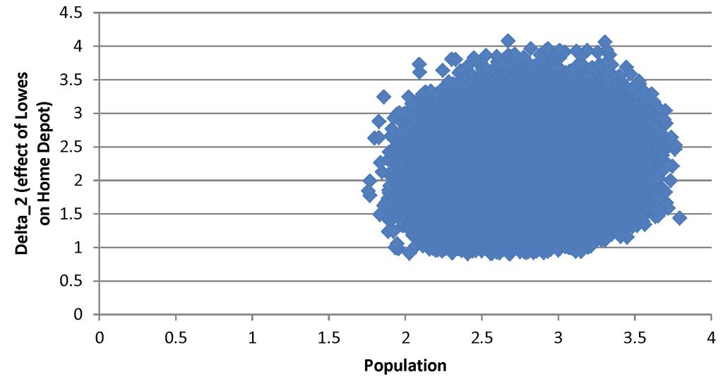
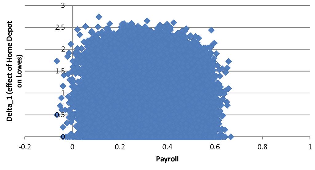
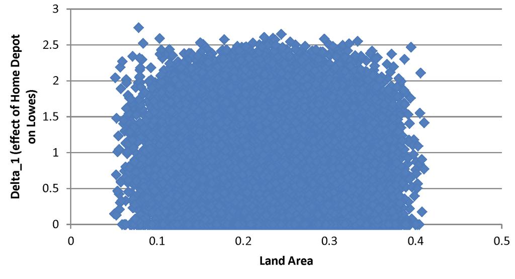
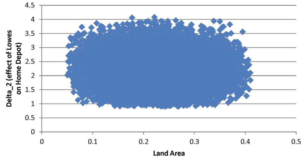
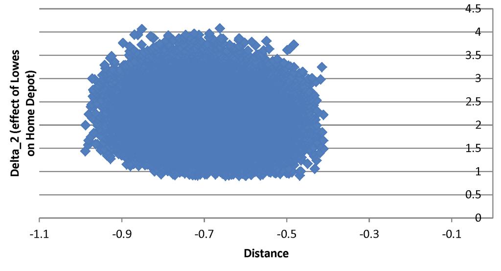
63 Figure 5: Joint 95% confidence region for strategic interaction coefficients and slope parameters 62

64 Figure 6: Confidence sets for estimated propensities of equilibrium selection (A) Equilibria with at most one store by each firm (B) Equilibria with a monopolist opening multiple stores (C) Equilibria where both firms enter with the same number of stores 63