Eulerian-Lagrangian Modeling of Particle Mixing in Gas Fluidized Beds

Transcription

1 Eulerian-Lagrangian Modeling of Particle Mixing in Gas Fluidized Beds Master of Science Thesis of Master Degree Program of Innovative & Sustainable Chemical Engineering AFARIDEH BABADOOST Department of Chemical & Biological Engineering Division of Chemical Reaction Engineering CHALMERS UNIVERSITY OF TECHNOLOGY Göteborg, Sweden, 2011

2

3 Eulerian-Lagrangian Modeling of Particle Mixing in Gas Fluidized Beds Master of Science Thesis of Master Degree Program of Innovative & Sustainable Chemical Engineering AFARIDEH BABADOOST Department of Chemical & Biological Engineering Division of Chemical Reaction Engineering CHALMERS UNIVERSITY OF TECHNOLOGY Göteborg, Sweden, 2011

4 MASTER S THESIS 2011 Eulerian-Lagrangian Modeling of Particle Mixing in Gas Fluidized Beds Master s Thesis in the Master s program of Innovative & Sustainable Chemical Engineering AFARIDEH BABADOOST Department of Chemical & Biological Engineering Division of Chemical Reaction Engineering CHALMERS UNIVERSITY of TECHNOLOGY Göteborg, Sweden, 2011

5 Eulerian-Lagrangian Modeling of Particle Mixing in Solids-gas Fluidized Beds Master s Thesis in the Master s program of Innovative & Sustainable Chemical Engineering AFARIDEH BABADOOST AFARIDEH BABADOOST, 2011 Master s Thesis 2011 Department of Chemical & Biological Engineering Division of Chemical Reaction Engineering CHALMERS UNIVERSITY of TECHNOLOGY Göteborg, Sweden, 2011 SE Göteborg Sweden Telephone: +46(0)

6 Eulerian-Lagrangian Modeling of Particle Mixing in Solids-gas Fluidized Beds Master s Thesis in the Master s Program Innovative & Sustainable Chemical Engineering AFARIDEH BABADOOST Department of Chemical and Biological Engineering Division of Chemical Reaction Engineering ABSTRACT The diploma work concerns Eulerian-Lagrangian modeling of particle mixing in gas-solid fluidized beds. That has a great influence on the performance of fluidized-bed combustors. Better horizontal and vertical mixing yields homogenous cross-sectional tracer distribution in the furnace and secures long enough contact time between oxygen and the tracer particles. To understand the motion of the two particulate phases (inert bed material) suspended in a fluid, the Lagrangian particle tracking technique is used. This study contains numerical modeling of mono disperse particles mixing in spouted beds and fluidized beds in different beds dimensions. Formulating a suitable statistical procedure for analyzing the results obtained and results were evaluated based on schematic comparison of tracer particles concentration and degree of mixing in specific regions of the bed; moreover, preferential position, which states about the general distribution and tendency of particles to move across the regions of bed during mixing time, velocity vector and horizontal dispersion patterns are obtained to investigate about the mixing in the beds. The numerical study is done in open source software for simulating fluid dynamics of fluidized beds (MFIX), The code was developed at the National Energy Technology Laboratory (NETL), USA. Key words: MFIX, Fluidized bed, Lagrangian simulation, Multiphase numerical modeling I

7 Table of Contents Preface... IV List of Figures... V List of Tables... IX Nomenclature... X 1 Chapter One Introduction Gas-solid flows Continuity & momentum equations Solid-phase, Discrete Element Method (DEM) Drag force Void fraction Solid-phase velocity calculation Pressure Force/Buoyancy Calculation Collision in Discrete Element Method Hard Sphere model Soft Sphere model Particle-wall interaction: Particle-neighborhood search N 2 search Quadtree and Octree search No-Binary search Verlet-Neighbor List Linked-Cell (LC) Linked-Linear List (LLL) Chapter two: Solution method Convection-Diffusion term discretization Scalar transport equation discretization Source term Solution algorithm summarize Chapter Three: Results and discussions II

8 3.1 Sampling method Particle concentration & Mixing Index Case1: Mixing process illustration Case 2: Effect of various spouting gas velocity at distribution of tracer particles concentration Case 3: Effect of different fluidization velocities on tracer particles distribution General pattern-influence of spouted gas velocity Preferential position & velocity vectors Horizontal Dispersion General pattern- Influence of fluidizing gas velocity Preferential position and velocity vectors Horizontal Dispersion: Coclusion References: III

9 Preface In this work, Eulerian- Lagrangian numerical modeling of mono dispersed mixing in fluidized beds is performed using MFIX open source software at Division of Fluid Mechanics at Department of Mechanical Engineering, Chalmers University of Technology, Sweden. The diploma work is carried out from beginning of 2010 to beginning of 2011 by supervision of researcher, Meisam Farzaneh and advisor, Professor Srdjan Sasic at Department of Mechanical Engineering. Professor Bengt Andersson at Department of Chemical & Biological Engineering was examiner of this Master s Thesis work. Finally, I would like to have special thanks to Prof. Srdjan Sasic and Meisam Farzaneh, PhD, for their useful comments and support of this work at Multiphase group in Division of Fluid Mechanics. I am so thankful of my lovely parents and family and my loved one whom supported me by all means during studies and granted me the best encouragement. Göteborg, Sweden, February 2011 Afarideh Babadoost IV

10 List of Figures Figure 1.1 Figure 1.2 Figure 1.3 Figure 1.4 Particle-particle collision in hard sphere approach Particle-particle interactions in soft sphere model and displacement of δ Spring dashpot model used in soft sphere model definition Particle-wall collision and corresponding velocities which related to coefficient of restitution Figure 1.5 Sample of particle gridding in quadtree method of particle neighborhood search Figure 1.6 Figure 1.7 No-Binary Search method in finding neighbor cells Comparison among N 2, NBS, Quadtree and Octree in 2D searching method for particle size more than 1000 Figure 1.8 Figure 1.9 Figure 1.10 Figure 1.11 Figure 2.1 Figure 3.1 Verlet circles (2D)/spheres (3D) Linked cell methods in particle searching neighborhood LLL bounding boxes contain various particles Particles projection on x-axis in LLL neighborhood approach Control volume and node locations in 1D, x-direction Simple schematic view of the flatted-bottom spouted bed and Fluidized bed used in the simulation Figure 3.2 Schematic view of sampling regions corresponding to the tracer areas in the bed Figure 3.3 Mixing procedure and variation of mean concentration of tracer particles with time in cells U, N, X Figure 3.4a Axial distribution of tracer particles concentration in spouted-bed with 11cm width at different spouting gas velocities Figure 3.4b Axial distribution of tracer particles concentration in V

11 spouted-bed with 15cm width at different spouting gas velocities Figure 3.4c Axial distribution of tracer particles concentration in a spouted-bed with 21cm width at different spouting gas velocities Figure 3.5a Radial distribution of tracer particles concentration with various spouting gas velocities in spouted-bed with width of 11 cm Figure 3.5b Radial distribution of tracer particles concentration with various spouting gas velocities in spouted-bed with width of 15 cm Figure 3.6a Mixing index in spouted-bed with width of 11 cm and various spouting gas velocities in radial and axial directions Figure 3.6b Mixing index in spouted-bed with width of 15 cm and various spouting gas velocities in radial and axial directions Figure 3.6c Mixing index in spouted-bed with width of 21 cm and various spouting gas velocities in radial and axial directions Figure 3.7a Axial tracer particles concentration distribution in various fluidizing gas velocities in given spouting gas velocity of U s /U ms = 1.1 in a fluidized bed with width of 11cm Figure 3.7b Axial tracer particles concentration distribution in various fluidizing gas velocities in given spouting gas velocity of U s /U ms = 1.1 in a fluidized bed with width of 15cm Figure 3.7c Axial tracer particles concentration distribution in various fluidizing gas velocities in given spouting gas velocity of U s /U ms = 1.1 in a fluidized bed with width of 21cm Figure 3.8a Radial distribution of tracer particles concentration in various fluidizing gas velocities and given spouting velocity of U s /U ms =1.1, in fluidized bed with width of 11cm VI

12 Figure 3.8b Figure 3.8c Radial distribution of tracer particles concentration in various fluidizing gas velocities and given spouting velocity of U s /U ms =1.1, in fluidized bed with width of 15cm Radial distribution of tracer particles concentration in various fluidizing gas velocities and given spouting velocity of U s /U ms =1.1, in fluidized bed with width of 21cm Figure 3.9a Mixing index at various fluidizing velocities and defined spouting gas velocity of U s /U ms =1.1, in fluidiezed bed with 11 cm width Figure 3.9b Mixing index at various fluidizing velocities and defined spouting gas velocity of U s /U ms =1.1, in fluidized bed with 15 cm width Figure 3.9c Mixing index at various fluidizing velocities and defined spouting gas velocity of U s /U ms =1.1, in fluidized bed with 21 cm width Figure 3.10 Figure 3.11 Figure 3.12 Figure 3.13 Figure 3.14 Figure 3.15 Effect of spouting gas velocity on preferential position of tracer particles in bed with width of 11 cm Velocity vector with increase in spouting gas velocity in fluidized bed with width of 11 cm Effect of spouting gas velocity on preferential position of tracer particles in bed with width of 15 cm Velocity vector with increase in spouting gas velocity in fluidized bed with width of 15 cm Effect of spouting gas velocity on preferential position of tracer particles in bed with width of 21 cm Velocity vector with increase in spouting gas velocity in fluidized bed with width of 21 cm VII

13 Figure 3.16 Figure 3.17 Figure 3.18 Figure 3.19 Figure 3.20 Figure 3.21 Figure 3.22 Figure 3.23 Figure 3.24 Figure 3.25 Horizontal dispersion with increase in spouting gas velocity in fluidized bed with width of 11 cm Horizontal dispersion with increase in spouting gas velocity in fluidized bed with width of 15 cm Horizontal dispersion with increase in spouting gas velocity in fluidized bed with width of 21 cm Effect of fluidization velocity with constant U s /U ms =1.1 on preferential position of tracer particles in bed with width of 11 cm Effect of fluidization velocity with constant U s /U ms =1.1 on velocity vector of tracer particles in bed with width of 11 cm Effect of fluidization velocity with constant U s /U ms =1.1 on preferential position of tracer particles in bed with width of 15 cm Effect of fluidization velocity with constant U s /U ms =1.1 on velocity vector of tracer particles in bed with width of 15 cm Effect of fluidization velocity with constant U s /U ms =1.1 on preferential position of tracer particles in bed with width of 21 cm Effect of fluidization velocity with constant U s /U ms =1.1 on velocity vector of tracer particles in bed with width of 21 cm Horizontal dispersion with constant U s /U ms =1.1 and increasing fluidizing velocity Figure 3.26 Horizontal dispersion with constant U s /U ms =1.1 and increasing fluidizing velocity in fluidized bed with width of 15 cm Figure 3.27 Horizontal dispersion with constant U s /U ms =1.1 VIII

14 and increasing fluidizing velocity in fluidized bed with width of 21 cm List of Tables Table 3.1 Table 3.2 Physical properties of solid bed materials set in MFIX simulation Dimension of fluidized beds with relevant number of particles and tracer particles IX

15 Nomenclature Roman Upper Case Letters C d F s F sml F gm Empirical Drag coefficient Solid drag force Drag coefficient between m th and l th solid phase Drag coefficient between gas and m th solid phase Inter-particle collision force Normal force Net sum of forces acting on the i th particle Total contact forces between particles Total drag force on i th particle belonging to the in k th cell and in the m th solid phase G 12 Relative velocity at particle centroids Interaction force of momentum transfer between gas and m th solid phases Interaction between m and l phases of solid (solid- solid momentum transfer) I (i) Momentum inertia of i th particle Impulsive force vector exerted on particle 1 Sliding collision Sticking collision Number of particles in phase mth solid N P jm Total number of particles in Lagrangian tracking Pressure of particle j in m th solid phase Particle Reynolds number Mass transfer interphase X

16 Mass transfer interphase R ml R 0m Mass transfer from m th to l th phases of solids Mass transfer from gas to the m th solid phase Gas phase stress tensor m th solid phase stress tensor Vvelocity of particle i of m th phase in cell j U smj V smj Volume averaged solid velocity of m th solid phase in cell j Total solid volume fraction of m th solid phase in cell j Volume fraction of a particle i of m-th size solid phase in fluid cell j V j V j V m Cell volume Particle volume Total particles volume in the cell Particle s linear velocity Particle s position Roman Lower Case Letters d (i) Particle i diameter Particle diameter e n Coefficient of normal restitution e t Coefficient of tangential restitution Internal porous surface force k n m (i) Stiffness factor Mass of particle i Normal velocity Unit normal between particle i to j XI

17 Tangential velocity Δt Computational time step Fluid velocity Greek Letters β Interphase momentum exchange coefficient δ Overlap displacement δ ij Overlap displacement between particles i and j ɛ g Volume fraction of fluid phase (Void fraction) ɛ sm Volume fraction of m th solid phase ɛ smj ɛ sj Volume fraction of particle i of m th size solid phase in fluid cell j Total volume fraction in the cell ɛ j Volume fraction in j th cell ɛ m Solid phase volume fraction η Damping coefficient f Coefficient of friction Fluid viscosity ρ g Fluid density ρ sm m th solid phase density ρ (i) υ p 1 Particle s density Particle velocity after collision with wall Fluid velocity m th solid phase velocity Relative velocity of particles i and j Particle s angular velocity XII

18 1 Chapter One 1.1 Introduction The purpose of this thesis is numerical modeling of Eulerian-Lagrangian solid particles mixing in fluidized bed with MFIX (Multiphase Flow with Interphase exchanges). MFIX is multipurpose software developed by National Energy Technology Laboratory (NETL), USA. MFIX is written in FORTRAN; it is a hydrodynamic modeling tool uses for chemical reaction and heat transfer modeling in various types of solid-fluid flows, dealing with energy and mass conservation, gives accurate time-dependant information on pressure, temperature, composition and velocity distribution of phases [1]. Stability, speed up calculation and accuracy in calculation are factors in high importance in every modeling. MFIX enhances two first factors by replacing old-iterating method with two modified extension of SIMPLE (semi-implicit scheme); first, to enhance the solid convergence when solids are poorly packed with help of equation of solids volume fraction correction instead of solids pressure correction. Second, uses automatic timestep alteration to enhance the highest speed executes. The latter factor, accuracy, discretization convection term is altered to the second-order upwind [2]. Gas-particle flow is a dominant concept on design and formulation of MFIX. Therefore, we review the governing solids-gas flow equations, particle and fluid tracking approach in Eulerian- Lagrangian framework, Discrete Element Simulation (DES), Drag force criteria, collision and etc. Following to that, computational method to solve practically formulations in designing and programming MFIX is discussed. 1.2 Gas-solid flows The controversial concept of gas-solid flows is described by strong coupling between fluid and particles. Fluid flows through voids formed by solid particles. A drag force exerted mutually from gas to solids and from solids equally and opposite to the gas. Therefore, pressure gradient arises that makes press forces on the particle phases. This phenomenon accompanied with different density of phases which causes buoyancy driving flows, makes energy and momentum exchange between two phases. 1

19 1.3 Continuity & momentum equations Hydrodynamic motions of gas -solid phases are defined by generalized spatially outlined Navier- Stokes equations for two-phase flow mixtures. Gas and solid continuity and momentum equations description categorized in two definite groups of Eulerian-Eulerian and Eulerian- Lagrangian approaches, which are briefly and respectively, are discussed. General gas continuity equation is: (ɛ g ρ g ) + ɛ g ρ g υ ) = (1.1) Solid continuity equation defined as for m th solid phase: (ɛ sm ρ sm ) + ɛ sm ρ sm υ ) = (1.2) The terms on the right side of equations (1.1) & (1.2) stand for mass transfer interphase due to chemical reaction and/or physical processes such as evaporation [3]. This term is zero in cases where there is no chemical process considered in the fluidized bed [4], [10]. Momentum equations used for gas phase in general form is: (1.3) (ɛ g ρ g υ ) + ɛ g ρ g υ υ ) = + ɛ g ρ g + represents gas phase stress tensor and is interaction force of momentum transfer between gas and m th solid phases, internal porous surface insert force of [3]. Momentum equation for solid phase (m th solid phase) is: 2

20 (1.4) (ɛ sm ρ sm ) + ɛ sm ρ sm υ υ ) = + ɛ smg ρ sm - + In momentum equation of m th solid phase, is result of interaction between m and l phases of solid (solid- solid momentum transfer) as described by: = F sml (υ υ ) + R ml [ ξ mlυ + mlυ ] (1.5) In equation (1.5), R ml is mass transfer from m th to l th phases of solids and so, where R ml, then ξ ml = 0 and where R ml < 0 ξ ml = 1. Moreover, lm = 1- ξ lm. The major interaction forces in fluidized beds are drag force, buoyancy and momentum transfer caused by mass transfer. Solid-fluid interaction force concluded as: = - ɛ g g F gm (υ υ ) R 0m [ ξ 0mυ + 0mυ ] (1.6) In equation (1.6) the first term on right side is buoyancy, second is drag force and third term describes momentum transfer due to mass transfer between gas and solid phases, where R 0m describes the mass transfer from gas to the m th solid phase which split when R 0m 0 then ξ 0m = 0, and when R 0m < 0 then ξ 0m = 1. Similarly, 0m = 1- ξ 0m. To close the above equation, solid stress tensor is required but the formulation of kinetic theory used in MFIX is replaced by DES so, there is no need for this closure. In favor of using DES, solids continuity equation and solids momentum equations are omitted. Continuum simulation is coupled with DES; so that, solids volume fraction and solids velocity are directly calculated in order to find the exact position and velocity of particles. As a result, particles should be located in each gas computational cell [3]. 1.4 Solid-phase, Discrete Element Method (DEM) 3

21 In DEM simulation, particles are tracked individually. Particles are categorized and packaged based on diameters and densities so that create various solid phases. For example, m th solid phase is individualized by N m spherical particles with each particle in diameter d m and density ρ sm. Summation total number of M solid phases gives the total number of particles, N, which represents Lagrangian approach: N = (1.7) At time t these N particles which stated are representative of Lagrangian framework are referenced by set of vectors as {,,, d (i), ρ (i), i = 1,, N}. These vectors denote respectively as particle s position, particle s linear velocity and particle s angular velocity, d (i) represents particle s diameter and ρ (i) is particle s density. In Lagrangian tracking, density and diameter of each particle is same as m th solid phase stated before. Following equations are used to describe the mass (m (i) ) and momentum inertia (I (i) )of the i th particle are respectively [10]: m (i) = ρ (i) π (d (i) ) 3 /6 (1.8) I (i) = m (i) (d (i) ) 2 /10 (1.9) Based on the MFIX documentation, following equations are defined to calculate linearly the position and angular velocities of i th particle, respectively [10]: = (1.10) m (i) = = m (i) + (1.11) I (i) = (1.12) Equation (1.11), is net sum of forces acting on the i th particle and consisted of gravity force, which is the total drag force, consists of pressure and viscose forces on i th particle 4

22 belonging to the in k th cell and in the m th solid phase; also, particles. is total contact forces between Two main forces which dominates gas-solid motion are interphase drag and pressure force or buoyancy. Although, other interactive forces, such as, Basset force, Magnus lift force etc. could be considered Drag force Drag force is a result of energy dissipation at the particle surface and corresponds to the fluid mean velocity related to that of the particle. Hoomans et al. and Kawaguchi et al. illustrate forces act on a single particle as [4], [6]: m p = m p + ( - ) - (1.13) In equation (1.13), the second term represents drag force and β stands for an interphase momentum exchange coefficient is obtained by Ergun equation. Drag force in high Reynolds number follows by empirical correlations and becomes non-linear function of related fluidparticle velocities [5]. Hoomans et al. state β, for ɛ < 0.80, is [3], [4], [9]: β = (1- ɛ ) - (1.14) For low volume fraction, Ergun equation is not sufficient; therefore, for ɛ 0.8, Wen and Yu presented the following equation for C d, which is an extension of Richardson and Zaki formulation [4]: C d = C d ρ g - ɛ (1.15) In empirical correlations, drag coefficient, C d is a function of Reynolds number [4], [5], [7]: C d = ( Re p ) Re p < Re p 1000 (1.16) And particle s Reynolds number calculated as [4], [5], [7]: 5

23 Re p = (1.17) Kuipers et al. suggested a correlation for drag force on a single particle in a particulate flow [3], [8]: F s = 1/8 C d π d p 2 ρ f (1.18) C d and Re in equation (1.18) calculated based on equation (1.16). Different suggestions are made for. Wen and Yu has suggested simple function of = ɛ - 4.7, Felice correlation which introduces parameter α in calculation of = ɛ α and α = exp [ - ] when 2 < Re < 500. Happel introduced another correlation, = [3]. In calculation of drag force utilized in MFIX, terminal velocity of the m th solid phase is used. In all above equations, term of volume fraction was used. Volume fraction of fluid continuum and solid phase needs to be calculated which is described later in Void Fraction section. Grag et al. has stated about numerical errors happen in obtaining accurate value for intephase momentum transfer. They believe it could be arise to particle locations by approximation of fluid velocity at grid nodes. As a result, different numerical schemes suggested and manipulated in order to improve numerical algorithm for computation interphase momentum transfer [16] Void fraction Domain of fluid continuum phase is meshed to computational cells. Each particle enters and exits from each cell and total value of all particles volume in each cell is solid volume fraction. Total solid volume fraction of m th solid phase in cell j represented by V smj is calculated by following equation: V smj = (1.19) While V pimj is volume fraction of particle i of m-th size solid phase in fluid cell j. When cell volume is V j = ΔxΔyΔz, corresponding volume fraction is: ɛ smj = (1.20) 6

24 V j components are width of the cell in x-cartesian direction, also in y and z directions. By summation each phase solid particle s volume fraction in the cell, the total volume fraction in the cell is obtained: ɛ sj = (1.21) In view of the fact that sum of various solid void fraction and fluid volume fraction is equal to one, volume fraction in j th cell obtained by: ɛ j = 1 - ɛ sj (1.22) Solid-phase velocity calculation In Lagrangian tracking approach, it is needed to calculate each particle size group velocity. This velocity is a factor in calculation drag force and should be computed in each fluid cell; therefore, at the end of solid time step, each particle s velocity in the cell is calculated and all averaged. In order to have representative of solid velocity in each cell, these velocities are averaged in each cell and stored in the cell center, and give volume averaged solid velocity of m th solid phase in cell j according to the following equation: U smj = (1.23), is a velocity of particle i of m th phase in cell j. This velocity as stated, stored at center of cell while numerical schemes use the face center value. Thus, the related neighbor cells center velocity should be weighted averaged crossed the face Pressure Force/Buoyancy Calculation At each fluid time step the fluid continuum equation is solved and fluid properties like pressure and velocity is obtained. This pressure exerted from fluid to each individual particle in the cell and stored in the cell center. For the particle j in m th solid phase P jm is given by: P jm = ɛ m P c (1.24) 7

25 Where, ɛ m = (1.25) In (1.24), V j is particle volume, V m is total particles volume in the cell and ɛ m is the solid phase volume fraction. 1.5 Collision in Discrete Element Method In DES approach, particle-particle interaction and particle-wall interaction is considerable and loss of kinetic energy due to inter-particle collision in non negligible. Two models Hard Sphere Model and Soft Sphere Model are two common approaches utilized. Hard sphere model is quasi-instantaneous binary collision based on event driven approach and soft sphere model is modeled with spring-dashpot model. DES is based on soft sphere model since it is more robust because of independence to the time step size from volume fraction. Energy released during collision affects coefficient of restitution while restored in elastic deformation connected with normal and tangential displacement of contact points corresponding to the sphere s center [11] Hard Sphere model Particle-particle collision in this approach is inelastic and time step is established based on minimum collision time between each two pairs of particles. This is analogous to mean free path. This approach is more suitable for dilute systems since the time step is much smaller than denser systems where particles collide with each in very short time scale. Due to inelasticity of this approach, energy will be re-supplied to the system. In hard sphere modeling, particles move in a defined path and trajectories till collision with other particles happen. Figure 1.1 can visualize hard sphere model. 8

26 Figure 1.1 Particle-particle collision in hard sphere approach [3] Hard sphere model is based on impulsive forces which are integration of forces acting on the particle versus time. Equations below can define modeling by hard sphere approach [9]. If two particles with velocities of υ 1 and υ 2 have relative velocity υ 12 at contact point, then this velocity is defined as: = ( ) ( r 1 r 2 ) (1.26) In equation (1.26), and are angular velocities and r 1, r 2 are radii of particle 1 and particle 2. Normal and tangential velocities, and are calculated by: = (1.27) = (1.28) Where subscription 0 points out state before collision and G 12 indicated relative velocity at particle centroids. Equations (1.29), (1.30), (1.31) and (1.32) are equations of motion for particles where I 1 and I 2 are introduced as moments of inertia and is impulsive force vector exerted on particle 1. Followed, various coefficients important in hard sphere modeling with related formulas are introduced. These coefficients are coefficient of normal restitution e n, coefficient of friction f and coefficient of tangential restitution e t. m 1 ( ) = (1.29) m 2 ( ) = (1.30) ( ) = (1.31) 9

27 ( ) = (1.32) I with indices 1 and 2 is I = (2/5) ma 2 [12]. Coefficient of restitution, e n calculates with equation (33): = m 1 m 2 (1+ e n ) (1.33) Coefficient of friction and coefficient of tangential restitution are representative of two collisions, sliding and sticking. Conditions, in which these collisions are valid, specified by following equations: = - f if f < (1.34) = - if f (1.35) Soft Sphere model In various studies the need of modeling collision with soft sphere model is discussed and numerical investigations in DEM modeling using soft sphere model validated with experimental modeling of particles behavior in gas fluidized beds. Rhodes et al. stated that soft sphere model consumes much CPU time when modeling large dense beds especially when simulating particles with large spring constants is performed [13]. Voigt model which models springs and dashpots that has ability to be used in contact point of several particles with one particle is investigated; while, integration time step should be particularly smaller than interactions of particles duration in this type of modeling [14]. Soft sphere modeling starts with calculation of contact force exerted on particle a, which is sum of all contact forces from contact list particles of this particle such as wall and all particles named b. = + ) (1.36) The right hand side parameters in equation (1.36) states, the normal and tangential forces respectively between particles a and b. The torque is dependent on tangential force and defined by equation (1.37) as below: = ) (1.37) 10

28 It is always tried to describe contact mechanism by a model which reduces the calculation time while provides the procedure with high accuracy; the simplest model originally suggested by Cundall abd Strack [7]. This model describes contact force by linear-spring and dashpot model shown in Figure 1.3. In this model, the normal contact force between particles a and b is described by combination of k n, normal spring stiffness, the normal unit vector, η n, the normal damping coefficient, the normal relative velocity and overlap, δ n. The contact force between two particles a and b is: k n δ n - η n (1.38) Figure 1.2 Particle-particle interactions in soft sphere model and displacement of δ [3] Figure 1.2 shows the concept of displacement, δ n, which is calculated as follows: δ n = (1.39) The normal relative velocity is calculates by equation (1.40): =(. (1.40) The normal damping factor acquired in calculation of normal contact force, is given by: η n = if e n and η n = 2 if e n = 0 (1.41) In equation (1.41), m ab =(1/m a + 1/m b ) -1 and coefficient of normal restitution, e n is defined as. = e n (. It is needed also to calculate the tangential force by its components of Coulomb-type friction law [7]: k t δ t - η t when μ μ when >μ (1.42) Tangential spring stiffness, tangential displacement and tangential damping coefficient is described respectively as follows: 11

29 η t = if, and η n = 2 if = 0 (1.43) In both components of equation (1.43), is the friction coefficient and its calculation is stated by Deen et al. (2007)[7]. The tangential displacement is described as: δ t = δ t,0 + dt if μ and δ t = if >μ (1.44) Components of δ t, such as is defined in research work by Deen et al. (2007)[7]. Normal Force Tangential Force Figure 1.3 Spring dashpot model used in soft sphere model definition [3] 1.6 Particle-wall interaction: Particle-wall interactions are considered as two particles interaction with some modifications added, therefore, particle j is replaced by wall and = 0. One idea is to assume a reflecting wall. So, particle s velocity which contacted wall is related to coefficient of restitution. Initial velocity of particle in absence of wall is υ p 0 and traveling distance of υ p 0 Δt after contact with wall and stay in domain. Δt 1 is time for particle travels to the wall and after collision will remain inside the domain after distance of υ p 0 (Δt - Δt 1 ). After contact, the velocity of particle is υ p 1 = υ p 0 e (1.45) And total distance particle traveled would be υ p 0 Δt 1 + υ p 1 (Δt - Δt 1 ). This idea is depicted in Figure

30 Figure 1.4 Particle-wall collision and corresponding velocities which related to coefficient of restitution [3] Other suggestions of a scheme for particle-wall interaction are considered such as replacing neighbor j with wall. Another idea is periodic boundaries in large particle systems. Studies give another option such as irregular bouncing based on impulse equations for particle-wall interaction and gives higher value for particle velocity fluctuations which meets the experimental results better while movement of smaller particles are less affected by type of particle-wall collision model chosen [17]. 1.7 Particle-neighborhood search Collision detection is a sophisticated algorithm to find neighbor particles especially for large systems with wide range of particle size distribution. Some methods will be introduced in this section such as N 2 search, Quad-tree and Octree, No Binary Search, also other alternatives such as Verlet-Neighbor List (VL), Linked Cell (LC) and Linked Linear List (LLL) will be discussed N 2 search This algorithm is the easiest way to search neighbors. The neighbors are found based on calculation the distance between particles, this approach utilizes O(N 2 ) that N is the number of particles. It is not suitable for large-scale simulations due to expensiveness and generally is not recommended any more while other accurate methods uses now. 13

31 1.7.2 Quadtree and Octree search This is hierarchical structure in 2D modeling and its 3D modeling concept is Octree. Recursively, Quadtree splits a cubic volume into four cubes which is eight in Octree procedure. These smaller cubes are called quadrants and Octants in 2D and 3D simulation respectively and divide until the decomposition norm achieved to get maximum resolution desired. Meshing method is producing equal size boxes to store the data. Using such grid method, unnecessary data will be stored but quadtree gives more promising results in storing data and operation. Figure 1.5 shows one sample of quadtree meshing of a particle which is separate from effect of other particles. quadtree method is used for meshing the objects and providing O(NlogN) algorithm in subjective point neighborhood search. In Octree method the query is arranging particles in quads which maximum of four particles could be allocated then searching for neighbors. This quad is known as parent quad. If fifth particle lies down in the quad then it divides to four sub-quads, called children quads and old particles allocate into new children quads. This procedure continues till a vacant position is found. Next step is finding the neighbor. Therefore, a search region generates around the particles in a shape that all neighbor particles of interest should fall into this region and consequence of quadtree should be passed through and eliminating all the particles lay out of this search region. Therefore, in a moment that a quad meets the search region, the particles in quads start searching for neighbors. 14

32 Figure 1.5 Sample of particle gridding in quadtree method of particle neighborhood search [ In completion quadtree and octree particle neighborhood search, other methods are introduced for large amount of nodes stored in these methods [20]. Diffusion-limited Aggregation is an algorithmic structure used to determine the distance with help of DLA clusters with ability of distance searching between 10 9 in 2D simulation and 10 8 particles in 3D modeling. DLA upgraded to PDLA, a fractal cluster with ability of neighbor search among and 10 9 particles in 2D and 3D simulation respectively. Algorithm in Diffusion-limited Aggregation is an iterative process that included of a seed particle in its origin in form of initial cluster. A particle far from the origin moves randomly toward the cluster, this particle is in distance usually called, birth radius, R bh. It becomes part of the cluster when its distance to the origin is in a specific area. If the particles locate in boundaries exceeding R dh then it is discarded. When certain number of particles established in the process, then it is ended. One challenge is that all particles in a cluster should be aware of other particles in the cluster and their distances [20]. 15

33 1.7.3 No-Binary search As per its name, No-binary Search is not engaged in any binary search and involved O (N) algorithm search. This algorithm is only suitable for systems of same-size particles [27]. The domain for neighbor searching first split in a cell which just one particle can fit into, then integrized into x, y and z zones and represented by ix, iy and iz coordinates. Only particles with integrized coordinate of ix-1, ix, ix+1, iy-1, iy, iy+1, iz-1, iz, iz+1 could be searched for neighborhood list. Any combination of these integrized points could be detected to find neighbor particles. Figure 1.6 shows a schematic overview of neighbor search in NBS method. Figure 1.6 No-Binary Search method in finding neighbor cells [3] Figure 1.7 shows a comparison between N 2 search algorithm, NBS, Quadtree and Octree neighbor search algorithms in 2D simulation for over 1000 particle size in logarithmic scale. Quadtree, octree and NBS are in some orders of magnitude quicker than N 2 searching method. While, NBS seems faster than quadtree and octree but since NBS is a searching method between particles of equal sized, in DES simulation quadtree and octree are more reliable for neighborhood searching. 16

34 Figure 1.7 Comparison among N 2, NBS, Quadtree and Octree in 2D searching method for particle size more than 1000 [3] Following to general-used algorithm discussed previously, other methods are also available for mostly large-scaled systems and preferably with different-sized particles that is discussed as follows [28] Verlet-Neighbor List In this method an imaginary sphere with radius of five times more than maximum particles radius drawn [21]. It is shown in Figure 1.8. Particles which fall in these spheres are considered as neighbor to the particle in the center of that sphere. Densities of the entire system in line with velocity of particles also, are key factors to determine the optimum extension of this zone. A list of neighbors created for each particle and particle of higher numbers than the body itself are tested regardless of their location inside or out of the sphere region. Therefore, n (n-1)/2 calculation steps are required and number of necessary 17

35 operation is still in order of O (n 2 ). The neighborhood list will not be updated and it depends on density of the system, sphere sizes and particles velocity [21][22]. Figure 1.8 Verlet circles (2D)/spheres (3D) [21] Linked-Cell (LC) The domain is splited in to lattices like m m m cubic (3D).Non cubic lattice is also available. Optimal size of the cells are similar to VL method, described before but the imaginary cells are not attached to the particles and not moving with them [21][23]. In LC one cell can be determined that contains three particles. So, particles which are allocated in a same cell based on their position at the specific time interact with each other. (3 d +1) /2 cells will be examined for neighborhood which d=2 in 2D and d=3 in 3D cases. Figure 1.9 shows LC method. Figure 1.9 Linked cell methods in particle searching neighborhood [21] 18

36 1.7.6 Linked-Linear List (LLL) Linked Linear List method is different from the last methods of VL and LC and it is a useful method to keep track of particles neighbors in large body systems. Each particle is located in a box that exactly fits in and the sides of bounding boxes are lined with axis as shown in Fig In each time step particles location are projected on the x axis according to the length of their bounding boxes. Figure 1.11 shows this projection for Figure 1.10 each time step this projection differs. It happens a lot that beginning or ending or the whole projection of some particles overlap with others and in all time steps the overlapping calculations should be updated [21][24]. Figure 1.10 LLL bounding boxes contain various particles [21] Time t Time t + Δt Figure 1.11 Particles projection on x-axis in LLL neighborhood approach [21] 19

37 Particles collision are determined based on the projection list and rules defined to identify the colliding particles when their projections interfere with each other and results of neighboring are stored in a sparse matrix where colliding bounding boxes are stored. Further studies has improved Verlet-List and inked-cell approaches and combined the advantages of both models to lower the computational time and iterations; also to reduce the construction of neighbor list.the result is an improved neighbor list in order of O (N); data sorting and algorithm of cell decomposition is arranged to reduce the time and maximize the speed and reducing the unnecessary operation in reconstruction the neighbor lists [25][26]. 20

38 2 Chapter two: Solution method This chapter describes the computational method used in MFIX 2.0, which is provided by MFIX Documentation Numerical Technique by Madhava Syamal (1998) [2]. To provide more stability and speed in computation, SIMPLE (SemiImplicit Method for Pressure Linked Equations) developed that utilizes automatic time-step adjustment for pressure-velocity coupling. Two major modifications done in new version of MFIX regarding use of SIMPLE method; first, when solids packed loosely, solid volume fraction correction equation helps convergence instead of solids pressure correction equation; moreover, in dense packed solids, this equation brings up with solids pressure. Second, the high speed performance guaranteed by automatic time-step modification. Second-order upwind scheme is added to MFIX in order develop the precision in discretizing convection terms and error reduction (e.g. in predicting rounded shape for bubbles). Finite volume is the numerical technique used in MFIX for the gas phase. The domain split to control volumes (CV) containing large number of particles that momentum, continuity equations, balance of energy and species exerted in CVs. MFIX utilizes structured mesh in 2D or 3D. Diffusion and convection terms solved by second-order upwind descritization scheme and various second-order limited method used for convection term. The value of all scalars is stored at cells centroid, in addition to the gas and solids pressure. Gas and solids velocity is stored at cell face [3]. 2.1 Convection-Diffusion term discretization Convection-diffusion term in transport equation in 1D condition is defined as: (2.1) Figure 2.1 shows control volume in x-direction. Integration this term over rectangular control volume gives: = [ ] A e - [ ] A w (2.2) Which second-order accuracy scheme uses to calculate the diffusive flux at the east face according to equation (2.3) = + O ( (2.3) 21

39 Figure 2.1 control volume and node locations in 1D, x-direction [3] Value of ϕ at convection term is written as in equation (2.4) at east face and at west face according to equation (2.5): = (ξ e + ) (2.4) = (ξ w + ) (2.5) ξ e is weighting factor, that = 1- ξ e, value for weighting factor differs when u e 0 then ξ e =0 and when u e < 0, ξ e =1 and consequently, = 1- ξ w when u w 0 then ξ w =0 and when u w < 0, ξ w = Scalar transport equation discretization Scalar ϕ in transport equation should be descritized and all terms, convection, diffusion and transient term in equation (2.6) should be integrated over control volume. + = + R ϕ (2.6) The complete integrated form of each term is described in literatures; such as, calculation of diffusive fluxes at east face and use set of a harmonic mean of values for cell center calculation [3]. 22

40 2.3 Source term Generally, source terms are nonlinear and become linear as in equation (2.7), in this equation for stability reason, R ϕ ' 0. R ϕ (2.7) - R ϕ ' Integration equation (2.7) over control volume gives equation (2.8) and further combination and rearrangement gives equation (2.9) for ϕ. ϕ ϕ (2.8) a P = + b (2.9) nb represents as E,W,S,N,T and B. Discretized continuity equation multiply by ϕ needed to be subtracted from equation (2.9); therefore, set of coefficients defined as below: a E =D e - ξ e (u m ) e A e (2.10) a W =D w + (u m ) w A w (2.11) a N =D n ξ n (υ m ) n A n (2.12) a S =D s + (υ m ) s A s (2.13) a T =D t ξ t (w m ) t A t (2.14) a B =D b + (w m ) b A b (2.15) a P = +a p 0 + ϕ (2.16) b = a p 0 + (2.17) a 0 p = Δ V (2.18) Therefore, the diffusion contribution achieves as D e = (2.19) Consequently, the concluding discretized form of diffusion is: a P = + b (2.20) 23

41 To increase stability in computation procedure, under-relaxation changes during iteration should be provided for field variables as described in equation (2.21): That, 0 < < 1. Set of linear equation solvers are suggested in MFIX; such as, conjugate gradient and GMRES solvers with preconditions [3]. 2.4 Solution algorithm summarize Nature of gas-solid is unstable. In most of the cases, the transient modeling and results are timeaveraged. If the time step is too large, the transient simulation diverges and too slow time step makes simulation slow. So, MFIX automatically adjusts the time step [2]. A computational technique outline is suggested for each fluid time step [3]: 1. At the start of time step, rates of reactions, physical properties and also, exchange coefficients should be computed 2. Based on current pressure field, u m *, w m *, υ m *, fluid velocity field should be computed 3. P ' g stands for fluid pressure correction calculated 4. Under relaxation applied to renew field pressure; P g = ω pg P ' g + P * g 5. In this step, using fluid pressure correction P ' g, fluid velocity field updates as: u m = u m * + u m ' 6. Numerous gas phase iteration is needed to fulfill the appropriate convergence criterion 7. Now, DES-sub stepping starts; multiple solid time steps is utilized for a single fluid time step. Then at each solid time step following procedure should be completed: a) Calculation of contact forces; particles-wall interaction and inter-particles interactions b) Gas drag force exerted on every single particles should be computed c) Calculation of pressure force on every particles completes d) For each particles, new position, new velocity and acceleration computes 8. Now, the DES-sub stepping is over; with the results, solids volume fraction and void fraction in each computational cell computed. Solids velocity also calculated and the obtained results should be fed into MFIX. 9. Drag force applied from solids on the fluid should be calculated through gas-phase source term in this step 10. By achieving simulation time step, simulation stops otherwise it starts over from Step 1. 24

42 Convection terms should be discretized accurately, stable and have less oscillation. In order to have higher accurate and fewer spurious oscillation, a limiter is added to the discretization scheme; such as, second order scheme, third order accurate scheme ultraquick, Smart, Superbee, Muscl, Van Leer, Minmod, FPFOI, etc. are added to MFIX[37][38]. Superbee is a higher order scheme chosen due to its ability to predict the rounded shape of bubbles but the CPU time requirement for Superbee is the highest among other limiters stated above specially has given better results than second order discretization scheme. 25

43 3 Chapter Three: Results and discussions In this work numerical investigation of mono dispersed systems of spherical particles, in a flatten-bottom spouted bed and then in a fluidized bed is performed. Tracer particles and bed materials have the same diameter but slightly different density. Numerical modeling of beds are two dimensional with different cross-sections of beds, 11 m, 15cm and 21cm with 0.50m height. The results are obtained by simulation with MFIX codes (Multiphase Flow with Interphase exchange). The results will be compared with the visual, experimental study on spouted bed by Jin et al[29]. Spouted bed is categorized as a nonconventional fluidized bed. Some important parameters in modeling a spouted bed are minimum spouting velocity, spouted diameter and ratio of nozzle-toparticle diameter (D i /d p ), etc. Also, Sphercity and internal angle of friction are influential parameters in particle size distribution [30]. Number of particles, position of particles and preferential arrangement of the particles in binary systems can improve the mixing efficiency of fluidized beds [31]. This work divided to four main parts; part one, sampling method, part two, particle concentration and mixing index, part three, general pattern-influence of spouting gas velocity, part four, general pattern-influence of fluidizing velocity. Figure 1.3 is a simple schematic view of the flatted-bottom spouted bed and fluidized bed used in the simulation. Figure 3.1 simple schematic view of the flatted-bottom spouted bed and fluidized bed used in the simulation 26

44 3.1 Sampling method The solid particles peculiarities manipulated as the bed material in the simulation are presented in the Table 3.1. Table3.1 Physical properties of solid bed materials set in MFIX simulation Diameter, d p (m) Density,ρ p (kg/m 3 ) Voidage, ɛ Restitution coefficient Boundary conditions set in the modeling divide the whole bed to six sections; Distribution flow inlet at bottom that divides to three parts (gas-distributor plate at left, central jet, gas-distributor plate at right), the left side wall and right side wall and the exit at the upside of the bed. The dimensions of the bed mentioned before will satisfy the boundaries and 1 cm is considered for the central jet size. Initially, in the state of no air flow, the bed consisted of two layers of particles. Boundary conditions at distributor flow inlet, central gas jet which is located at the bottom of the bed (see Figure 3.1) is Mass inflow, at exit where located at top of the bed is Pressure outflow and at walls are Free slip wall. For better understanding of the mixing behavior of particles with inspiration of the experimental sampling method in spouted-bed used by Jin et al [29], the numerical sampling method elaborated based on the location of each particles saved during the mixing process. Data of all particles location are available every one second. Tracer particles position is also saved every 0.01 second, then the particles Cartesian (x,y) location is ready to use in the formulations which could give the particles concentration in specific areas in the bed. Axial and radial tracer particles concentration investigated. Figure 3.2 can help to identify the locations where particles included bed materials and tracers were detected [29]. 27

45 Figure 3.2 Schematic view of sampling regions corresponding to the tracer areas in the bed Blocks which are marked with alphabetic characters are specified to detect the particles in. Each block has width and length of 0.01m 0.02m. The regions U, V, N, W, X is located horizontally. 3.2 Particle concentration & Mixing Index Two parameters are important to calculate the concentration of particles; one, concentration of local tracer particles (c li ) and second, concentration of tracer particles (c) [29]. According to Jin et al. (2009): c li (3.1) c (3.2) Which n i represents number of tracer particles in a sampling cell, n it shows total number of particles in a given sampling cell and n t gives total tracer particles in the whole bed [29]. The mixing index employed by Jin et al. [29] used to define the degree of mixing, is given in equation (3.3), although various mixing indices are defined for this purpose [33]. So that, mixing index, M is defined the ratio: M (3.3) Which, σ (c) represents standard deviation that is function of local tracer particles concentration, therefore defined as: 28

46 σ (c li ) (3.4) Where, m represents number of sampling cells in the desirable system. is average concentration of tracer particles in the bed. The amount obtained is approximately 0.1, which is observed in the plot of c l vs. time, Figure 3.2. Through the simulation, different gas velocities are applied and effect of increasing velocity on various bed dimensions and tracers distribution and other results investigated. These velocities are calculated based on minimum spouting gas velocity (U ms ) and minimum fluidization velocity (U mf ) in equations (3.5) and (3.6)[30]. for D<0.5 m (3.5) for Ar <1000 and Re mf = Ar (3.6) In equation (3.5), D stands for bed width and H is considered as unit height. In equation (3.6), Ar number calculates based on Ar = that in our simulation case is less than Case1: Mixing process illustration To have visual and mathematical observation of particles mixing and flow pattern of bed materials, especially tracer particles, which act an important role in mixing of bed materials and segregation, a modeling performed with specifications of U f = 0 m/s, U s =1.4 U ms, the data obtained from this simulation could help to evaluate the mixing pattern of tracers by plot of mean concentration of local tracer particles by time. The sampling is done in three regions referred as U, N, X (Figure 3.2). Figure 3.3 illustrates various stages in mixing particles. According to this plot, with respect to time, mixing process could be separated into three sections. 29

47 c l Time (s) Figure 3.3 Mixing procedure and variation of mean concentration of tracer particles with time in cells U, N, X With deeper notice, three sequential mixing stages could be distinguished. Macro-mixing, Micromixing and Stable-mixing stage [29]. Details of these stages are as following: 1. Macro-mixing stage, which the spouted jet gas begins to penetrate into the bed, mixing is limited to the region inside the jet (internal jet). From Figure 3.2, a rapid steep of mean concentration from the beginning of mixing to 0.1 mean concentration which is referred to the average point of the tracers mean concentration. After 2 s of mixing, sudden falling off mean concentration detected which is followed by more slight steeps and change of mean concentration, and continues till mixing time of 10 s. velocity of mixing is high in this stage. 2. Micro-mixing stage, in which large particles mix with the bed materials. Driving force for this stage is spouted gas which penetrates through the whole bed and forms continuous circulation of particles. Dynamic equilibrium is close to reach in the next stage after micro-mixing stage ends in 15 s of mixing so this stage took 5 s. 3. Stable-mixing, forms after 15 s of mixing and steady state mixing observes. Degree of mixing basically does not change with time as in Figure 3.2 the fluctuations after 15 s which are strong but around the average amount of mean concentration of local tracers. This figure shows the dynamical equilibrium reaches after 15 s. It is worthy to notice that these results evaluate MFIX ability in modeling a spouted bed which is studied by Jin et al.[29]. Their results show 6 s of Macro-mixing stage and 6 s duration of Micromixing stage and finally the bed reaches dynamical state after 12 s. 30

48 Mostoufi & Chauoki [31] discussed mixing mechanisms and diffusivity in gas-solid fluidized beds. They described mixing of solid particles is underlying different mechanisms; Global mixing of solids which is caused by bubble-induced mixing that solid circulation occur due to the rising and bursting gas bubbled. Local mixing that is caused by random movement of solid particles Case 2: Effect of various spouting gas velocity at distribution of tracer particles concentration The axial distribution of tracer particles concentration with different spouting gas velocities are shown in Figure 3.4a, Figure 3.4b, and Figure 3.4c. As shown, the results are obtained along the bed height in regions of L, M, N, O, P, Q, R, S, T in Figure 3.2; at vertical coordinate the concentration of tracer particles calculated based on equation (59). In this case, there is no fluidized gas velocity (u f = 0 (m/s)) and spouting gas velocities at Us/U ms = 1.2, Us/U ms = 1.4, Us/U ms = 1.6. This evaluation is done in different bed widths of 11cm, 15cm and 21cm. In the lowest spouting gas velocity equals to minimum spouting gas velocity, generally amount of tracers concentration is higher in annulus region rather than fountain region. L, M, N, O and P are annulus regions; A dense region where is surrounding the spout and particles fall down in this region [29]. The rest of the referred regions are in fountain region where particles concentration is very low. According to Figure 3.4a, when the gas velocity rises up to 1.4u ms, concentration decreases more in annulus region in compare with the lower velocity (U s =1.2U ms ) and as it goes to the upper region, the fountain area, where, concentration increases. As velocity goes to U s = 1.6U ms, this trend particularly becomes infirm. The range of c (statically is the difference between minimum and maximum of a value) for different velocities implies that increasing in spouting gas velocity does not necessarily make increase in promotion axial mixing and shows an optimum for amount of increasing in spouting gas velocity. In Figure 3.4a, the lowest velocity has the highest value of concentration and after that the highest velocity shows higher concentration in various areas of the bed, but the general pattern remains same through different velocities that closer to the bottom bed shows more averaged concentration and as the vortexes in the bed, which bring particles upward, develop upward through bed, the concentration of particles decreases. This pattern is also applicable for Figure 3.4b and Figure 3.4c. By increasing the bed width which means increasing bed material in Figure 3.4b, the highest average concentration decrease in compare with Figure 3.4a. It could be interpreted that as the bed dimension increases in the same velocities, less particles pass across the same region in bed because they have more area to move so the concentration in specific areas of bed decreases by increasing the bed width and bed material. This conclusion makes sense when the bed width 31

49 C (Averaged Concentration) C (Averaged concentration) increases further to 21 cm in Figure 3.4c, that at the same velocity, the average concentration in Figure 3.4c is less than Figure 3.4b and Figure 3.4a Us/Ums=1.2 Us/Ums=1.4 us/ums=1.6 0 L M N O P Q R S T Region Figure 3.4a Axial distribution of tracer particles concentration in spouted-bed with 11cm width at different spouting gas velocities L M N O P Q R S T Region Us/Ums=1.2 Us/Ums=1.4 Us/Ums=1.6 Figure 3.4b Axial distribution of tracer particles concentration in spouted-bed with 15cm width at different spouting gas velocities 32

50 C (Averaged Concentration) C (Averaged Concentration) Us/Ums=1.2 Us/Ums=1.4 Us/Ums=1.6 0 L M N O P Q R S T Region Figure 3.4c: Axial distribution of tracer particles concentration in a spouted-bed with 21cm width at different spouting gas velocities Radial distribution of tracer particles is another factor to better understand the behavior of spouted beds and fluidized beds beside axial distribution of tracer particles. Radial distribution of tracers concentration in specific areas of U, V,N, W and X (according to Figure 3.2) is presented in Figure 3.5a,3.5b and 3.5c Us/Ums=1.2 Us/Ums=1.4 Us/Ums=1.6 0 U V N W X Region Figure 3.5a Radial distribution of tracer particles concentration with various spouting gas velocities in spouted-bed with width of 11 cm 33

51 C (Averaged Concentration) As per of Figure 3.5a, it is expected to have more concentration in region V. Slight increase in the concentration of tracers distinguishable from region U to X in U s /U ms =1.2 that higher concentration is in region X, near wall. It is difficult to compare the results by axial and radial mixing, but obviousely increasing spouting bed, increases degree of mixing in spouted bed. According to Figure 3.5a, as the sampling region moves closer the wall side, the tracers concentration increases. The highest value of concentration in radial distribution is observed in highest spouting velocity. The mentioned pattern is also observable in Figure 3.5b, the concentration distribution is less uniform than Figure 3.5a, and the highest value is this case is less than in Figure 3.5a. It may due to the fact that by increasing bed width, fewer particles may move across specific sampling areas in the bed, so the concentration of tracer particles decreases by increasing the bed width. As the velocity increases, more uniform tracer concentration distribution is observed in the bed. It makes sense in Figure 3.5c as well that by increasing bed width, the average concentration decreases in sampling regions. More uniform distribution of tracers concentration is observed as the bed width more increased to 21 cm in Figure 3.5c. As the spouting velocity increases, less averaged concentration got in the sampling regions more close to the bottom bed because higher velocity spreads the particles more upward and juts in the beginning of vortex formation and after descending vortexes, particles meet bottom bed regions. Still higher values of averaged concentration are observed in regions V and N U V N W X Region Us/Ums=1.2 Us/Ums=1.4 Us/Ums=1.6 Figure 3.5b Radial distribution of tracer particles concentration with various spouting gas velocities in spouted-bed with width of 15 cm 34

52 C (Averaged Concentration) Us/Ums=1.2 Us/Ums=1.4 Us/Ums=1.6 0 U V N W X Region Figure 3.5c Radial distribution of tracer particles concentration with various spouting gas velocities in spouted-bed with width of 21 cm Due to the importance of understanding degree of mixing in both axial and radial direction and comparing qualitative results, Figure 3.6a shows M (mixing index) vs. U s /U ms. Five regions in axial and radial directions are representative for degree of mixing. Mixing index are calculated accordimng to equations (3.3) & (3.4). In 2D simulation of spouting gas velocities, highest degree of mixing index in radial direction is more than axial direction. It is valid for all spouting gas velocities examined and presented in Figure 3.6a for a spouted bed with width of 11 cm. Forces on the particles can describe the reason. Both have same declining trend of mixing index by increasing spouting gas velocity. Greater value of radial mixing could be discussed that in spout region, around the center axis where particles move upward with higher velocity, the drag force due to spouting gas velocity on particle is more than inherent gravity so braodly developes axial mixing and give uniform mixing. In Figure 3.6a both axial and radial mixing decreses with increasing spouting gas velocity. That indicated increasing gas velocity enhances particle mixing in this examined bed. Further incerasing bed width to 15 cm, gives mixing index diagram of Figure 3.6b. In Figure 3.6b instable mixing index is observed that the axial mixing is dominant on radial mixing in lower velocities and then axial and radial indexes catch a same value when U s /U ms =1.4 and then by increasing velocity radial mixing takes higher value than axial mixing index and gives uniformity to the axial mixing. Increasing bed width to 21 cm in Figure 3.6c, gives interesting feature that shows radial mixing has more values than axial mixing, this pattern indicates that axial mixing has more uniformity. 35

53 M (Mixing Index) M(Mixing Index) 0.12 Axial Sample region: L,M,N,O,P Radial sample region: U,V,N,W,X radial axial Us/Ums Figure 3.6a Mixing index in spouted-bed with width of 11 cm and various spouting gas velocities in radial and axial directions 0.25 Axial sample region:l,m,n,o,p Radial sample region:u,v,n,w,x radial axial Us/Ums Figure 3.6b Mixing index in spouted-bed with width of 15 cm and various spouting gas velocities in radial and axial directions 36

54 M (Mixing Index) Axial sample region: L,M,N,O,P Radial sample region:u,v,n,w,x Us/Ums radial axial Figure 3.6c Mixing index in spouted-bed with width of 21 cm and various spouting gas velocities in radial and axial directions Case 3: Effect of different fluidization velocities on tracer particles distribution Changing spouting gas velocity to the fluidizing gas velocity will change the void fraction and particles velocity. Also, change of mixing pattern is expecting. So that, Figure3.7a, 3.7b and 3.7c can show the results of axial distribution of particles concentration in the same regions as Figure 3.4a,3.4b and 3.4c used in given spouting gas velocity of U s /U ms = 1.1 and diverse fluidizing velocities. Figure 3.7a general pattern on concentration distribution of particles is that high concentration observed at the bottom of bed and decreases to the higher regions. This pattern is common in all examined fluidizing velocities. Totally, incresing fluidizing gas velocities, increases axial mixing. Comparing axial mixing due to the fluidizing velocities in Figure 3.7a shows greater values for particles concentration in compare with axial mixing due to spouting gas velocity with the same bed in Figure 3.4a. This matter can aslo show the ability of MFIX software to model beds with fluidizing gas velocity conditions rather than spouting gas velocities. Higher values of tracers concentration happens by increasing the fluidizing velocity. Increasing bed width to 15 cm show less averaged concentartion of tracer particles in compare with smalerr bed due to the reason described for the same condition happens in spouting bed. In Figure 3.7b, the concentration decreases as the particles reach higher regions of bed but increasing velocity enhances particles concentration at the bed higher areas. 37

55 C (Averaged Concentration) C (Averaged concentration) Us/Ums=1.1 uf/umf=0.88 uf/umf=1.15 uf/umf= L M N O P Q R S Region Figure 3.7a Axial tracer particles concentration distribution in various fluidizing gas velocities in given spouting gas velocity of U s /U ms = 1.1 in a fluidized bed with width of 11cm L M N O P Q R S T Region Us/Ums=1.1 Uf/Umf=0.88 Uf/Umf=1.15 Uf/Umf=1.33 Figure 3.7b Axial tracer particles concentration distribution in various fluidizing gas velocities in given spouting gas velocity of U s /U ms = 1.1 in a fluidized bed with width of 15cm 38

56 C (Averaged Concentration) Us/Ums=1.1 Uf/umf=0.88 Uf/Umf=1.15 Uf/Umf= L M N O P Q R S T Region Figure 3.7c Axial tracer particles concentration distribution in various fluidizing gas velocities in given spouting gas velocity of U s /U ms = 1.1 in a fluidized bed with width of 21cm Figure 3.7c shows similar pattern of particles distribution in bed. As discussed the higher value of averaged concentration is less than previous cases. As fluidizing velocity increases through the bed, concentration decreases in the lower parts of the bed and increase close to the fountain region. Radial distribution with different fluidizing gas velocities is shown in Figure 3.8a, 3.8b and 3.8c. In Figure 3.8a, by increasing fluidizing velocity, the averaged value of concentration increases in radial coordinate. Particles concentration spreads more uniform by increasing velocity when scattered from center of bed to the wall, in region V and N degree of concentration is considerable. Increase in fluidization velocity makes rapid tracer particles movement and enhances higher diffusion of particles especially in annular area. In Figure 3.8b, the bed width is increased to 15 cm and average concentration value decreases in compare with Figure 3.8a. In lower fluidizing velocity higher concentration is observed in the centerline as particles and this pattern does not change significantly by moving to the wall. Increasing in the fluidizing velocity has reverse effect on the radial movement in compare with Figure 3.8a and leads particles to have more concentration in the centerline and near wall. By increasing bed width to 21 cm in Figure 3.8c, this pattern improves that more averaged concentration is found in close to the centerline of the bed and as the sampling region location moves to the wall side, the concentration decreases. Increasing fluidizing velocity decreases the highest value of concentration in radial coordinate. 39

57 C (Averaged Concentration) C (Averaged concemtration) Us/Ums=1.1 uf/umf=0.88 uf/umf=1.15 uf/umf= U V N W X Region Figure 3.8a Radial distribution of tracer particles concentration in various fluidizing gas velocities and given spouting velocity of U s /U ms =1.1, in fluidized bed with width of 11cm U V N W X Region Us/Ums=1.1 Uf/Umf=0.88 Uf/Umf=1.15 Uf/Umf=1.33 Figure 3.8b Radial distribution of tracer particles concentration in various fluidizing gas velocities and given spouting velocity of U s /U ms =1.1, in fluidized bed with width of 15cm 40

58 C(Averaged Concentration) Us/Ums=1.1 Uf/Umf=0.88 Uf/Umf=1.15 Uf/Umf= U V N W X Region Figure 3.8c Radial distribution of tracer particles concentration in various fluidizing gas velocities and given spouting velocity of U s /U ms =1.1, in fluidized bed with width of 21cm As comparison between axial and radial mixing features is complicated, mixing index is considered as a factor that leads to better understanding of the mixing phenomena throughout the bed. Mixing index related to bed width of 11 cm in depicted in Figure 3.9a. Just like the cases which only spouting gas velocity was present in the bed(figure 3.6a), in this bed radial mixing have higher value than axial mixing which indicates axial mixing gas advantage over radial mixing in bed with such condition in Figure 3.9a but the mixing index increases with increasing velocity. Figure 3.9b, is very similar to Figure 3.6b that uniformity is not observed in the bed. This bed with width of 15cm shows in lower fluidizing velocities, axial mixing is more dominant in the bed than radial mixing and this procedure reverses after radial and axial mixing meet the same value in the bed and afterward, the fluidizing velocity increases. Figure 3.9c shows bed mixing index with width of 21 cm; in contrast with results in Figure 3.9a and 3.9b, axial mixing is dominant than radial mixing in the bed. It concluded that radial mixing is more uniform than axial mixing; moreover, fluidizing velocity increases radial movement in annulus area which helps reaching uniformity consequently. By increasing velocity, radial mixing in a small range gets higher value than axial mixing and makes axial mixing more uniform and favorable in the bed. 41

59 M(Mixing Index) M (Mixing Index) Axial sample region: L,M,N,O,P Radial sample region: U,V,N,W,X Uf/Umf Radial Axial Figure 3.9a Mixing index at various fluidizing velocities and defined spouting gas velocity of U s /U ms =1.1, in fluidiezed bed with 11 cm width Axial sample region:l,m,n,o,p Radial sample region:u,v,n,w,x Uf/Umf axial radial Figure 3.9b Mixing index at various fluidizing velocities and defined spouting gas velocity of U s /U ms =1.1, in fluidized bed with 15 cm width 42

60 M (Mixing Index) Axial sample region: L,M,N,O,P Radial sample region:u,v,n,w,x Uf/Umf axial radial Figure 3.9c Mixing index at various fluidizing velocities and defined spouting gas velocity of U s /U ms =1.1, in fluidized bed with 21 cm width 43

61 3.3 General pattern-influence of spouted gas velocity Preferential position & velocity vectors This part related to statistical investigation on effect of different spouting gas velocities and different bed dimensions on velocity vectors and preferential position of tracer particles, in two dimensional beds with various width of 11 cm, 15 cm, and 21 cm which number of total particles and tracer particles vary in each cases. In chapters, 3.3 and 3.4, a statistical analysis procedure is defined in MFIX to obtain results of preferential position; this statistical analysis method is described as follows: 1. The computational domain is discretized into quadrangular parts 2. Information of tracer particles stored 3. Number of times that particles move into each element is calculated 4. Particles mean velocity in each cell calculates Table 3.2 shows number of total particles and tracer particles in each bed. Table 3.2 Dimension of fluidized beds with relevant number of particles and tracer particles Fluidized bed dimension Number of total particles Number of tracer particles (cm cm) Bi-dispersed modeling with inert bed materials of d p,inert = m and ρ p.inert = 900 kg/m 3, with particles treated as tracers in mixing with d p,inert = m, ρ p.inert = 905 kg/m 3 are used. This statistical analysis is done based on 50 seconds of bed performance. Figure 3.10 illustrates preferential position of tracer particles in a bed with dimension of 11cm 50 cm (10 cm bed material height). Effect of various spouting gas velocities of 1.2 U ms, 1.4 U ms and 1.6 U ms is investigated. Figure 3.10, Figure 3.12 and Figure 3.14, show general distribution and tendency of tracer particles to move across regions of the beds during mixing time. Although tracer particles move all around the bed but the regions where particles most of the time move through, are in areas with highest value if normalized concentration and as goes from top to bottom of legend of normalized concentration with attention to the legend, and lowest value indicates, the probability of moving tracer particles to those regions decreases [33]. Figure 3.10 shows effect of different spouting gas velocities on tracer particles preferential position. To describe the general pattern, as velocity increases, the height of the bed increases and in lower velocity red spots at the bottom corner of the bed illustrates intention of tracer particles to move to these areas which the red 44

62 spots eliminate by increasing velocity and gives more uniform concentration of tracer particles in the bed and less preferred zone is observed. (a) U s = 1.2 U ms (b)u s =1.4 U ms (c)u s = 1.6 U ms Figure 3.10 Effect of spouting gas velocity on preferential position of tracer particles in bed with width of 11 cm In Figure 3.10 the regions with less tracer particle concentration are more observant when the velocity increases in bed and ascending velocities of the tracer particles by matching with Figure In Figure 3.11(a), with the lowes velocity, one bubble path and two vortexes are indentified as vetrical channels and have lower tracer concentration and upward, higher velocities and velocity vector patterns also seen to have one main bubble path and two votexes as velocty incerase to Figure 3.11(b) and (c). 45

63 (a)u s = 1.2 U ms (b)u s =1.4 U ms (c)u s = 1.6 U ms Figure 3.11 Velocity vector with increase in spouting gas velocity in fluidized bed with width of 11 cm In Figure 3.11(a), highest concentration of fule particles is clear in rotational centerpoints in the created vortexes, which is close to the bottom bed surface. This pattern is eliminating as spouting gas velocity increases. In Figure 3.11(c), the regions with highest tracers concentration is suppressed and less major than Figure 3.11(a). The same general pattern described for Figure 3.9 and 3.10, could be observed for Figure 3.12, 3.13, 3.14 and In Figure 3.12 and 3.14, with increase in velocity the bed develops but comparing these two figures with Figure 3.10, dense bed gradually with increase the bed size and bed velocity eliminates. The flow regime shows dilute core and denser regions close to the walls, which is more sever in Figure 3.14(c). In the central part of this regime, solid and gas flow directed upward and make solid dense enough to throw the tracers upward, therefore the tracer region moves upward in the central region and moving downward in the denser region of the walls. Increasing the bed width means increase in the total number of particles which is bed material included tracer particles. 46

64 (a) U s = 1.2 U ms (b)u s =1.4 U ms (c) U s = 1.6 U ms Figure 3.12 Effect of spouting gas velocity on preferential position of tracer particles in bed with width of 15 cm In Figure 3.11, Figure 3.13 Figure 3.15,one main bubble path and two vortexes were created.it could conclude that number of vortexes and bubbles paths depend on amount of bed material and not to the fluidizing regime, in addition, the amount of bed material effects concentration and velocity field of tracer particles [34]. Figure 3.12 and Figure 3.14 shows that by increasing the bed width which in our cases means increasing amount of bed material consequently, the highest particle concentration value decreases. In Figure 3.12(c), and Figure 3.14(c), in compare with Figure 3.10(c) the core part of bed shows very low concentration of tracer particles in general and populates the tracers particles more at the bottom of the bed rather than central and upper parts. Tracking Figure 3.12 and Figure 3.14, individually, we notice that by increasing velocity, the tracer particles concentration decrease in central and upper parts and more concentration is observed at the bottom bed, but the highest value of concentration decreases by increasing the velocity, these results are more severe in Figure 3.14 with bigger width of bed of 21 cm and more bed inert materials. Also, considering Figure 3.13 and Figure 3.15, individually, it is seen that in all the figures, one main bubble path and two vortexes are observable even in lower 47

65 (a)u s = 1.2 U ms (b)u s =1.4 U ms (c)u s = 1.6 U ms Figure 3.13 Velocity vector with increase in spouting gas velocity in fluidized bed with width of 15 cm velocities and by increasing velocity, tracer particles enter a splash zone and spread up with higher velocity vectors. Again, these phenomena are more severe in Figure 3.14 and very strong mixing with highest velocity vectors happen in a bigger bed with width of 21 cm and U s /U ms = 1.6. In Figure 3.14 the concentration of tracer particles has higher value at the bottom of the bed, indicates that the tracer particles have more tendency to pass through this area and may segregate. Increasing in bed inert material leads to increase in velocity of tracer particles. Comparison in Figure 3.11 with Figure 3.13 and 3.15 even if in (a) cases in each figure, we conclude that velocity fields has higher value in bigger beds and even in same velocities in each case, the velocity fields in bigger beds, distributes in higher regions in the bed (note the change in scales). 48

66 (a)u s = 1.2 U ms (b)u s =1.4 U ms (c)u s = 1.6 U ms Figure 3.14 Effect of spouting gas velocity on preferential position of tracer particles in bed with width of 21 cm (a) U s = 1.2 U ms (b)u s =1.4 U ms (c)u s = 1.6 U ms Figure 3.15 Velocity vector with increase in spouting gas velocity in fluidized bed with width of 21 cm 49

67 3.3.2 Horizontal Dispersion Mixing of particles plays a great role in the performance of spouted and fluidized beds. Gas-solid mixing in beds caused by different mechanisms; such as, global mixing and local mixing of particles. The former causes due to the net circulation of solids in the bed because of gas-bubbles rising up and bring the solids to the surface; bubbles burst and disperse the particles then descent to the bottom of the bed in form of emulsion, this mechanism called bubble-induced mixing which is illustrated by the bubbles movement. Parallel to the global mixing, local mixing of solids happen when the bubbles rise and between emulsion. This mixing is characterized by the random movement of solid particles. Both the mechanisms could be described by Fick s law within diffusion with different diffusion coefficients know as dispersion coefficient for the global mixing and particle diffusivity for the local mixing [34]. Local mixing and particle diffusivity described by Brownian movement, wall interaction and appraised by the random walk theory based on Lagrangian coordinates on set of particles [35-37]. Johansson et al. (2006) suggested a method to calculate local dispersion coefficient through experimental work. They implemented equation (3.7) to calculate local solid dispersion coefficient, as [34]: D k,n = (3.7) With k=x, y and for n= 1,..., N. Δt n is calculated based on the shutter time of the video camera which is stated generally in order of 10-2 seconds or lower. And Δl k,n is the change of displacement from one video frame to another. High values of Δt n increase the risk of underestimation of dispersion coefficient [34]. Figure 3.16 shows horizontal dispersion for bed with width of 11 cm. Figure 3.16(b) and 3.16(c) are similar in respect of general pattern of local dispersion and the lowest and highest value for dispersion in the bed. Highest value of dispersion should match with areas where bubbles burst. Figure 3.16(a), showed one main bubble paths and two vortexes, the highest dispersion value in the middle of this picture and some spots in the surface of the bed is observable. Bubbles lead the particles to the surface and when burst and erupt, spread the particles around and make the locations when maximum of horizontal dispersion happens. In Figure 3.16, the more noticeable dispersion locations are close to the sidewalls, where then particles were pushed to the middle of the bed which is the region where one main path are recognized and have less dispersion and more concentration of particles. Increasing the spouting gas velocity in Figure 3.16, approves a great effect of velocity on horizontal dispersion that make more uniform bed in this aspect and change the highest value of horizontal dispersion from Figure 3.16(a) to (b) and (c). 50

68 The pattern of horizontal dispersion which described for Figure 3.16 is observable in Figure 3.17, with increase in value of horizontal dispersion. It indicates that by increasing bed material even in the same velocity, the horizontal dispersion increases extensively. Particles are more uniformly spread in the bed in Figure 3.17(a), (b) and (c). Moreover, as the velocity increases, the height of bed basically increases. Still the regions with maximum amount of dispersion are close to sidewalls, where the vortexes and particles descend and circulate to form the new vortex in the bed. Figure 3.18 is a bed with width of 21 cm that the bed material is more than the last case. Generally, the highest value of dispersion is more increases in compare with cases in Figures 3.16 and Figure Notice to the change of scale shows that dispersion happens in higher regions in the bed. The pattern for horizontal dispersion considered close to the feature to the previous cases that more value of horizontal dispersion is observable in the sidewalls where the vortexes and particles descend. Special pattern is observed when velocity increases; more formation of bubbles happen in Figure 3.18(b) and (c) so the vortexes rise and speed up more than other cases and move particles upward then spread more to the sidewalls as seen in Figure 3.18(c) severely. Note that value of horizontal dispersion is much more than other cases. To conclude, by increasing the amount of bed material, dispersion coefficient value increases generally and severely along the sidewalls. Along center of the bed where the vortexes move upward and share a path together, horizontal dispersion is noticeable. By increasing the velocity, horizontal dispersion increases. 51

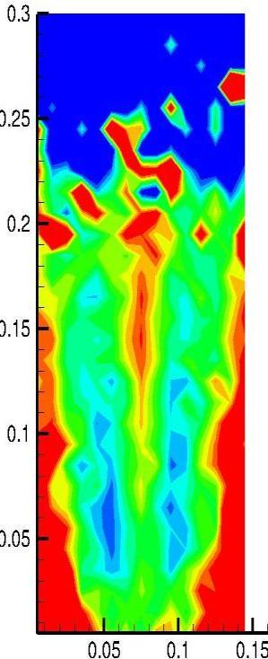
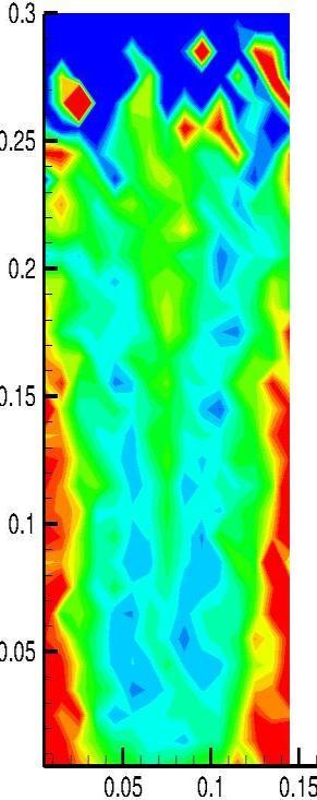
69 (a)u s = 1.2 U ms (b) U s =1.4 U ms (c)u s = 1.6 U ms Figure 3.16 Horizontal dispersion with increase in spouting gas velocity in fluidized bed with width of 11 cm (a)u s = 1.2 U ms (b)u s =1.4 U ms (c)u s = 1.6 U ms Figure 3.17 Horizontal dispersion with increase in spouting gas velocity in fluidized bed with width of 15 cm 52

70 (a)u s = 1.2 U ms (b)u s =1.4 U ms (c)u s = 1.6 U ms Figure 3.18 Horizontal dispersion with increase in spouting gas velocity in fluidized bed with width of 21 cm 53

71 3.4 General pattern- Influence of fluidizing gas velocity Preferential position and velocity vectors Preferential position in Figure 3.19 shows the tendency of tracer particles to move more across those areas during circulation. In Figure 3.19(a), (b) and (c) the highest value of tracers concentration are observed in close to the bottom bed and sidewalls, which decreases with increasing velocity; these areas are parts which vortexes descend and particles settle down to start a new circulation of vortex. More uniform concentration of particles is appeared in bed with increasing velocity. In Figure 3.21, this pattern is distinguished but the highest value of normalized concentration decreases; in Figure 3.21(a), highest value of concentration is observable at the bottom of the bed and by increasing the velocity this pattern changes and distribution of tracer particles shape more uniform in the bed with less value of concentration. Increasing the bed width to 21 cm in Figure 3.23, shows more change in the tracer particles change of pattern that in Figure 3.23(a) like Figure 3.19(a) and Figure 3.21(a) highest value of concentration is seen that these areas eliminates gradually by increasing velocity. But with increasing the bed material and bed dimension, more bubbles rise upward and burst so it changes the circulation of tracer particles in bed; careful look at the Figure 3.23 shows the regions where tracer particles have less attended are more observable and these regions show where bubbles are present. In conclusion, by increasing the bed material, more bubbles form in even same velocities with increasing velocity, more uniform pattern of tracer particles distribution is observed and consequently, the bed height has increased considerably, but the highest value of concentration decreases. Considering velocity vectors which show bubbles formation in the bed that move particles upward and then descending particles with ending up the vortexes circulation; in Figure 3.20, four vortexes with two main paths is seen and by increasing velocity it gets clear shape to the one mail bubble path and two vortexes. In Figure 3.22 this pattern improves even in lower velocities and it shows by increasing the bed materials we can improve the velocity vector pattern in the bed and better mixing happen. By increasing velocity better mixing of tracer particles in bed is observable through two vortexes and one main path for bubble eruption and dispersing tracer particles to the wall side then particles move down with ending up the vortexes and segregate at the bottom bed to start new circulation of vortex. Increasing more the bed material with bed width of 21 cm in Figure 3.24 clears out more the effect of amount of bed material on the formation of bubbles, expansion and eruption of bubbles that simultaneously moves up particles and causes better mixing in the bed. Even in lower velocities, a clear main path and two vortexes are observable while increasing fluidizing velocity gradually gives more uniform and clear cut of vortexes that in different heights throw the tracer particles up and develop the mixing. 54

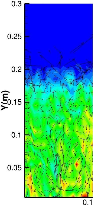
72 (a)u f = 0.88 U mf (b)u f =1.15 U mf (c)u f = 1.33 U mf Figure 3.19 Effect of fluidization velocity with constant U s /U ms =1.1 on preferential position of tracer particles in bed with width of 11 cm (a)u f = 0.88 U mf (b)u f =1.15 U mf (c)u f = 1.33 U mf Figure 3.20 Effect of fluidization velocity with constant U s /U ms =1.1 on velocity vector of tracer particles in bed with width of 11 cm 55

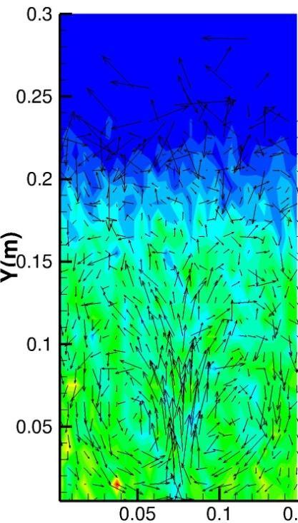
73 (a)u f = 0.88 U mf (b)u f =1.15 U mf (c)u f = 1.33 U mf Figure 3.21 Effect of fluidization velocity with constant U s /U ms =1.1 on preferential position of tracer particles in bed with width of 15 cm (a)u f = 0.88 U mf (b)u f =1.15 U mf (c)u f = 1.33 U mf Figure 3.22 Effect of fluidization velocity with constant U s /U ms =1.1 on velocity vector of tracer particles in bed with width of 15 cm 56

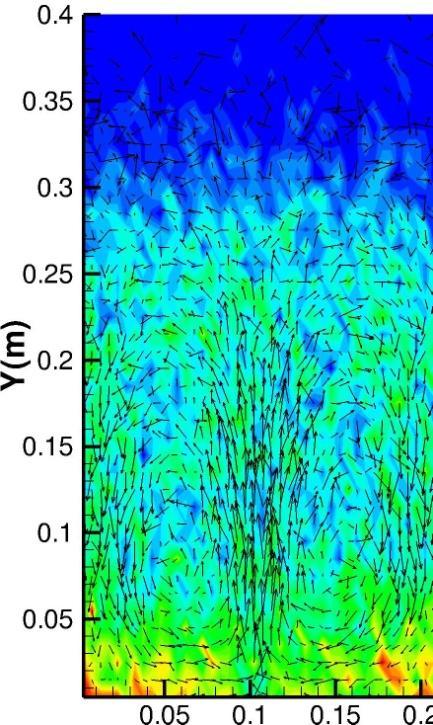
74 (a)u f = 0.88 U mf (b)u f =1.15 U mf (c)u f = 1.33 U mf Figure 3.23 Effect of fluidization velocity with constant U s /U ms =1.1 on preferential position of tracer particles in bed with width of 21 cm (a)u f = 0.88 U mf (b)u f =1.15 U mf (c)u f = 1.33 U mf Figure 3.24 Effect of fluidization velocity with constant U s /U ms =1.1 on velocity vector of tracer particles in bed with width of 21 cm 57

75 Comparing preferential position features and velocity vectors in figures with just spouting gas velocity and the others with presence of fluidizing velocity does not show large difference and the general pattern remains same in both cases, which may indicate that the most important parameter is bed material and superficial velocity of gas that spreads through the bed Horizontal Dispersion: Horizontal disperision as discussed before via the formulas suggested in litreature, indicates the tendency of particles to spread horizontally in the specific areas of the bed. In Figure 3.25, at lower fluidizing velocity, higher horizontal dispersion happens all along the wall. And less dispersion along the center line of the bed; by increasing fluidizing velocity, a v path appears and shows horizontal dispersion at the bottom corners and to some extend on the bed surface where vortexes descend and start to fall down. The dispersion regions are noticeably decreases with increasing fluidizing velocity in bed with width of 11 cm but the highest value of horizontal disperion increases gradually. In Figure 3.25(a) this pattern remains as more horzontal dispersion is observed in the surface and close to the walls at bottom bed. By increasing velocity, highest value for horizontal dispersion decreases. And gradually increasing the fluidizing velocity in Figure 3.25, shows increase in the regions of bed where tracers intend to disperse horizontally through the same pattern that close to the walls and in the center line tracer particles intend to disperse more. Increasing bed material to the bed with width of 21 cm shows increase in horizontal dispersion while particles gather more at the centerline of the bed and make less values of horizontal dispersion along the center line and more values of dispersion are observable at the wall sides, bottom bed and surface of the bed. This structure remains by increasing fluidizing velocity. Average value for horizontal dispersion increases but the large region assigned to less value of dispersion in Figure 3.25 (c). Average horizontal dispersion value is remained constant when comparing the results by just effect of spouting gas velocity with the cases with effect of fluidizing velocity. By increasing the ed length and fluidization velocity more uniform pattern of horizontal dispersion acheives. 58

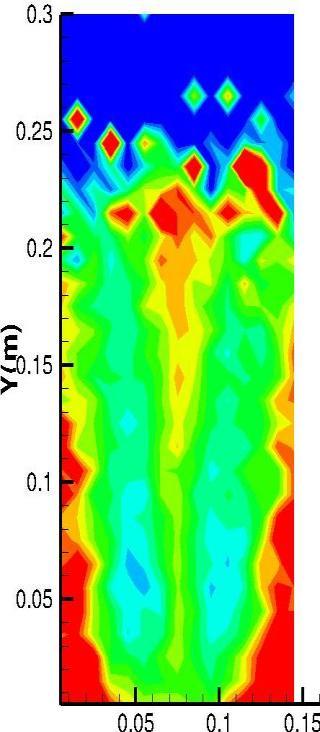
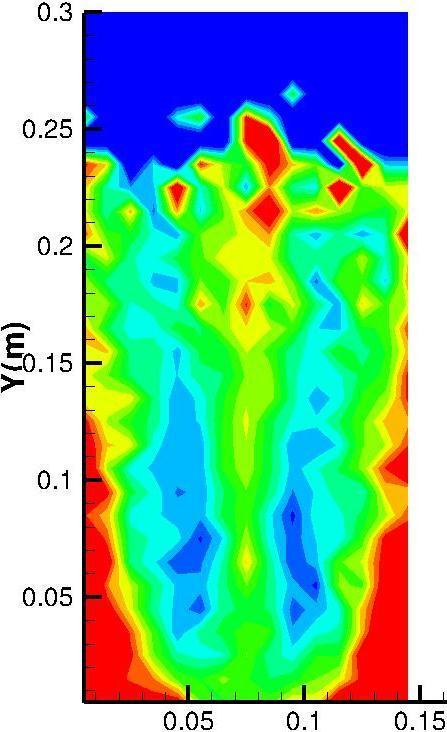
76 (a)u f = 0.88 U mf (b)u f =1.15 U mf (c)u f = 1.33 U mf Figure 3.25 Horizontal dispersion with constant U s /U ms =1.1 and increasing fluidizing velocity in fluidized bed with width of 11 cm (a)u f = 0.88 U mf (b)u f =1.15 U mf (c)u f = 1.33 U mf Figure 3.26 Horizontal dispersion with constant U s /U ms =1.1 and increasing fluidizing velocity in fluidized bed with width of 15 cm 59

77 (a)u f = 0.88 U mf (b)u f =1.15 U mf (c)u f = 1.33 U mf Figure 3.27 Horizontal dispersion with constant U s /U ms =1.1 and increasing fluidizing velocity in fluidized bed with width of 21 cm 60