Mean field coupling of expanding circle maps

Transcription

1 Department of Stochastics, TU Budapest October 2, 205.

2 Motivation José Koiller and Lai-Sang Young. Coupled map networks. Nonlinearity, 23(5):2, 200. Bastien Fernandez. Breaking of ergodicity in expanding systems of globally coupled piecewise affine circle maps. Journal of Statistical Physics, 54(4): , 204.

3 The coupled map system Phase space: T Dynamics: F µ = d Φ µ, where Φ µ (x) = x + ε 0 g(y x) dµ(y) mod (coupling) d(x) = 2x mod (site dynamics) 2 g(u) u

4 ( F µ (x) = 2 x + ε 0 ) g(y x) dµ(y) mod 0 ε Consider the system (F µ0, T). Let µ = (F µ0 ) µ 0. Then consider (F µ, T), and let µ 2 = (F µ ) µ... Question. lim t µ t =? Question 2. lim T T T t=0 µ t =? Question 3. "long-time behaviour of µ "?

5 Singular initial measure Initial measure: µ 0 = N δ xi. N i= Dynamics: ( ) F µ0 (x) = 2 x + ε N g(x i x) N i= mod. The pushforward of µ 0 : µ = (F µ0 ) µ 0 = N N δ Fµ0 (x i ). i=

6 A dynamical system on T N Consider the map ( (F ε,n (x)) s = 2 x s + ε N ) N g(x r x s ), s {,..., N}, r= x = (x s ) N s= T N. Piecewise affine map of T N. Expanding if ε < 2. finite number of ergodic acims (µ F ) with basin almost all of T N with densities in BV, see for example B. Saussol. Absolutely continuous invariant measures for multidimensional expanding maps. Israel Journal of Mathematics, 6(): , or D. Thomine. A spectral gap for transer operators of piecewise expanding maps, 200.

7 Each circle (x,..., x N ) + (t,..., t) mod is mapped onto another such circle (y,..., y N ) + (t,..., t) mod by stretching to twice its size then covering it twice. Ergodic components contain full such circles. The invariant density is actually constant on such circles. From this we can get, that the marginals of µ F have constant density, hence they are Lebesgue.

8 A(T ) = T (δ x,...,x N + + δ F T ε,n (x,...,x N ) ) µ F Because the marginals of µ F are Lebesgue (denoted by λ). A(T ) i = T (δ x i + + δ F T (x i )) λ. T µ t = T T t=0 T t=0 + N ( N N i= N δ xi + N δ N F (xi ) +... i= i= ) = N A(T ) i λ N δ F T (x i ) for Lebesgue a. e. x = (x i ) N i= TN. i=

9 Ergodic properties of (F ε,n, T N ) F 0,N is ergodic and mixing w. r. t. λ λ, F ε,n : a perturbation of F 0,N, F ε,n has a unique ergodic and mixing invariant measure if ε < ε 0 (N), for some small ε 0 (N), see G. Keller C. Liverani. Uniqueness of the SRB measure for piecewise expanding weakly coupled map lattices in any dimension. Communications in Mathemathical Physics, 262()33 50, Question: Is it true that there exists some ε (N), such that for ε > ε (N) the system fails to be ergodic (mixing)?

10 Breaking of ergodicity is only visible in the perpendicular direction to the main diagonal of the hypercube. New coordinates: u = N x s mod, s= u i+ = x i x i+ mod, i =,..., N We get a factor of the original system: G ε,n (u ) = 2 n (F ε,n (x)) s = 2u mod s= G ε,n (u i+ ) = (F ε,n (x)) i (F ε,n (x)) i+ mod, i =,..., N

11 { x, x + N,..., x + N } N share the same u-coordinates. G ε,n u : doubling map, invariant measure is Lebesgue G ε,n u2,...,u N : piecewise affine map of T N, expanding if ε < 2 : finite number of ergodic acims with basin almost all of T N with densities in BV, see again Saussol, Thomine. Acims of (G ε,n, T N ): µ G = λ ν

12 N=2, expanding case: 0 < ε < 2 F ε,2 (x, y) = (2x + εg(y x), 2y + εg(x y)) mod, x, y T. Notice: u = x + y 2(x + y) mod, u 2 = x y 2(x y) 2εg(x y) mod. Factor dynamical system: (x, y) ( x + 2, y + 2 G ε,2 (u, u 2 ) = (2u, 2u 2 2εg(u 2 )) mod, u, u 2 T. )

13 H(u 2 ) = 2u 2 2εg(u 2 ) mod The map H is conjugate with a linear Lorenz map of slope 2( ε). H(u 2 ) L(u 2 ) ε ε ε ε u 2 u 2

14 Theorem (Glendinning-Sparrow, 993) If a Lorenz map is not renormalizable, then it admits a unique mixing acim with support [0, ]. Theorem (W. Parry, 979) Let 2n+ 2 < 2( ε) < 2 n 2. A Lorenz map L with slope 2( ε) is n times renormalizable, R k L = L 2k Jk, 0 k < n, and the renormalizalion intervals form a nested sequence around 2 : 2 J k J k J J 0 = [0, ].

15 Corollary The Lorenz map L admits an ergodic acim and its attractor A = i=0 Li ([0, ]) is the union of 2 n mixing components if for the slope 2n+ 2 < 2( ε) < 2 n 2 holds. Ergodic invariant measure of H: µ H (mixing if ε < the attractor is the union of 2 n mixing components if 2 2 n < ε < 2 2 (n+) holds. Ergodic invariant measure of G ε,2 : µ G = λ µ H. Proposition F ε,2 admits an ergodic acim ( it is mixing if ε < attractor is the union of 2 n mixing components if 2 2 n < ε < 2 2 (n+) holds. ) 2 2, the ) 2 2,

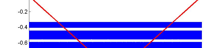
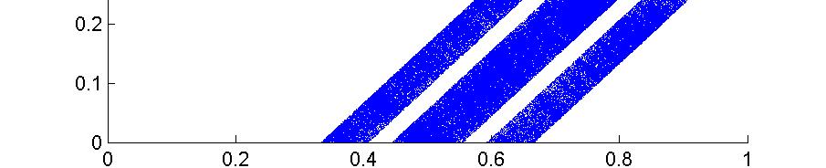
16 Example: ε = 3 Figure : G /3,2 and tiling. Figure 2 : F /3,2.

17 N=3, expanding case: 0 < ε < 2 Factor map: F ε,3 (x, y, z) = (2x + 2ε (g(y x) + g(z x)), 3 2y + 2ε (g(x y) + g(z y)), 3 2z + 2ε (g(z x) + g(y z))), 3 mod, x, y, z T. u x + y + z; u 2, u 3 x y, y z (x, y, z) ( x + 3, y + 3, z + ( 3) x + 2 3, y + 2 3, z + 2 ) 3 G ε,3 (u, u 2, u 3 ) = (G ε,3(u ), G 2 ε,3(u 2, u 3 )).

18 G ε,3 (u ) = 2u mod, u T, G 2 ε,3(u 2, u 3 ) = (2u + 2ε 3 (g(u 2) g(u + u 2 ) 2g(u ), 2u 2 + 2ε 3 (g(u ) g(u + u 2 ) 2g(u 2 ))) mod, u, u 2 T v u Figure 3 : Phase space of G 2 ε,3.

19 u=ε /3 v=δ u+v=σ v= ε /3 u= δ u+v=+ε /3 u+v= ε /3 u=δ v=ε /3 u+v=2 σ v= δ u= ε /3 u=v (VIb) (Vb2) (VIb) v= u/2+ (Ib2) (Ib) (Vb) (IIb2) (IIb) (IVb) (IIIb) v= 2u+ (IVb2) (IIIb2) v= 2u+2 (VIa2) (Ia2) (VIa) (Ia) (Va) (Va2) v= u/2+/2 (IIa) (IVa) (IVa2) (IIIa) (IIa2) (IIIa2) Figure 4 : The attractor and the invariant sets.

20 I = x=a,b k=,2 (Ixk),..., VI = x=a,b k=,2 (VIxk) Proposition If ε , then the sets I, II,..., VI are invariant with respect to the map G 2 ε,3. Corollary If ε 4 0 2, the dynamical system governed by the map F ε,3 does not have a unique ergodic acim, it has at least six ergodic components.

21 Figure 5 : ε = 0.2

22 Figure 6 : ε = 0.42

23 Let d be the quasimetric on T such that d(x, y) is the length of the counterclockwise arc from x to y. The invariant components correspond to the following type of states: I : II : III : IV : V : VI : {x, y, z S : d(x, y) < d(z, x) < d(y, z)}, {x, y, z S : d(x, y) < d(y, z) < d(z, x)}, {x, y, z S : d(y, z) < d(x, y) < d(z, x)}, {x, y, z S : d(y, z) < d(z, x) < d(x, y)}, {x, y, z S : d(z, x) < d(y, z) < d(x, y)}, {x, y, z S : d(z, x) < d(x, y) < d(y, z)}. Switch to the other hexagon: reverse the order of x, y, z on T N d(x, y), d(y, z), d(z, x) > ε 3

24 Contracting case: 2 < ε < N = 2: Gε,2 2 : 0 attracts every trajectory, F ε,2 : the diagonal x = y attracts every trajectory, and the map acts as the doubling map on it: the two sites synchronize N = 3: G 2 ε,3 : (0, 0) fixed point, ( 3, 3) ( 2 3, 2 3) periodic cycle attracts every trajectory. F ε,3 : an invariant circle, and two other circles mapped to each other give the attractor: either every site synchronizes, or the sites will be evenly placed on T and change order in each step.

25 N > 3 A T (x) = T (N ) T t=0 N ((Gε,N 2 )t+t 0 (x)) s? s= N = 4 and N = 5: A T A T ε ε Conjecture. There exists a threshold value ε(n) < 2, such that the system (F ε,n, T N ), ε(n) < ε < 2 has multiple ergodic components. These are related to the order of the distances between the sites: there are N! of them.

26 Absolutely continuous initial measure Let dµ = f dλ. Then ( F f (x) = 2 x + ε 0 ) g(y x)f (y) dy mod Let L Ff = L f. Then L f f (x) = y F (x) f f (y) F f (y). Let dµ 0 = f 0 dλ. Consider the system (F f0, T). Let f = L f0 f 0. Then let dµ = f dλ. Consider (F f, T), and let f 2 (x) = L f f... Question. lim t f t =? Question 2. "long-time behaviour of f "?

27 Let f C(T), dµ = f dλ. Facts about F f : F f C (T), Monotone increasing, Degree 2 covering map of T it has two invertible branches (the inverses of the branches will be denoted by y ( ), y 2 ( ))

28 The case of small ε Let f. Then F (x) = 2x mod and L f f (x) = ( ( x ) ( )) x + f + f = ( + ) = for all x T Theorem Let f 0 C (T) be a density such that f 0 TV δ. Assume that ε > 0 is such that ε < + 2δ. Then the density f of the pushforward measure (F µ0 ) µ 0 is in C (T) and has total variation for some c <. f TV c f 0 TV

29 Sketch of the proof: d L f f TV = 0 dx f (y)f f (y (x))y (x) (F f (y (x))) 2 Use that y F (x) f f (y) F f (y) + f (y 2 (x))y 2 (x) F f (y 2(x)) dx = f (y (x))y (x) 0 F f (y (x)) f (y)f f (y 2(x))y 2 (x) (F f (y 2(x))) 2 dx ( F f (x) = 2εf x ± ) 2 L f f TV + ε 2( εδ) 2 0 f (t) dt = + ε 2( εδ) 2 f TV

30 Case of large ε: strong coupling First we want to understand the sole effect of the coupling better. The coupling dynamics: Φ f (x) = x + ε 0 g(y x)f (y) d(y) mod. Let L Φf = L f be the associated transfer operator. We now calculate f = L f0 f 0, f 2 = L f f... Facts about Φ f : If f C(T), then it is a diffeomorphism of T, Monotone increasing.

31 Some limit behaviours Suppose f is supported on an interval of length 2 of mass if suppf [b, b 2 ]: on T. Center M(f ) = if suppf [0, b 2 ] [b, ]: M(f ) = b2 0 b2 b yf 0 (y) dy. (y + )f 0 (y) dy + yf 0 (y) dy b mod,

32 b M b 2 M b 2 b M + b 2 +

33 Let d be the quasimetric such that d(x, y) is the length of the clockwise arc from b to b 2. Proposition Let f 0 C(T) such that suppf 0 [b, b 2 ] or suppf 0 [0, b 2 ] [b, ], such that d(b, b 2 ) 2. The density f = L f f 0 is in C(T) and has support contained suppf [b, b 2 ], or suppf [0, b 2 ] [b, ], such that d(b, b 2 ) = ( ε)d(b, b 2 ), sup f = sup f 0 ε, M(f ) = M(f 0 )

34 sup f 0 ε sup f 0 f f 0 b b b 2 b 2

35 Proposition Let f 0 C(T) be 2 -periodic such that 0 xf 0(x) dx = 2. Then f C(T) is also 2 -periodic such that 0 xf (x) dx = 2, and f = ( ε) f 0, where denotes the constant function on T. 2

36 Back to F f and strong coupling Proposition Let f 0 C(T) such that suppf 0 [b, b 2 ] or suppf 0 [0, b 2 ] [b, ], such that d(b, b 2 ) 2. The density f = L f0 f 0 is in C(T) and has support contained suppf [b, b 2 ], or suppf [0, b 2 ] [b, ], such that d(b, b 2 ) = 2( ε)d(b, b 2 ), sup f = sup f 0 2( ε), M(f ) = 2M(f 0 ) mod

37 Note: 2( ε) if ε 2. sup f 0 2( ε) f sup f 0 f 0 b If ε = 2, then f is a translation of f 0 (on T). 2 b 2

38 Proposition Let 0 b < b 2 such that 2 < b 2 b < and let f 0 C(T) suppf 0 [b, b 2 ]. Let us assume that Let C = b2 2 0 f 0 (y) dy + f 0 (y) dy <. (T ) b (b 2 b ) 4 (b 2 b ) C ε <. The density f = L f0 f 0 C(T) has support contained in some interval [0, b 2 ] [b, 0] such that d(b, b 2 ) 2.

39 b b 2 b 2 2 b + 2

40 Summary of the absolutely continuous case Coupling dynamics (Φ f ): A well-concentrated initial distribution converges to a point measure supported on the center of mass. Certain symmetries in the initial distribution cause fast convergence to uniform distribution. Coupled dynamics (F f ): The density f is always invariant, other invariant densities exist when ε = 2. If ε is sufficiently small, the distribution converges the uniform. If ε is sufficiently large and the initial- distribution is well concentrated, the support of the distribution shrinks to a single point, while the center of mass shifts as the doubling map.

41 Thank you for your attention!

42 Coupling map: convergence to point mass when support is large Proposition Let f 0 C(T). Assume that f 0 (x) dx = xf 0 (x) dx = 2, 2 f 0 (x) dx = 2 The properties (S) and (S2) also hold for f = L f0 f 0. (S) (S2)

43 Proposition Let f 0 C(T) be such that f 0 (x) = f 0 ( x) for all x T. (S3) Then f = L f0 f 0 C(T) and also has property (S3).

44 Unimodal maps (P) f C (T), satisfies (S3) or (S) & (S2). (P2) f (0) = 0, f ( 2) = c(f ) > 0. (P3) f (0, 2) > 0, f (,) < 0. 2 If f 0 satisfies (P) (P3), then f = L f0 f 0 also satisfies (P) (P3). c(f ) = c(f 0) ε > c(f 0). 2 +δ f 0 (x) dx < 2 δ 2 +δ f (x) dx for all δ 2 δ ( 0, 2).