The comparison of stochastic frontier analysis with panel data models

Transcription

1 Loughborough University Institutional Repository The comparison of stochastic frontier analysis with panel data models This item was submitted to Loughborough University's Institutional Repository by the/an author. Additional Information: A Doctoral Thesis. Submitted in partial fulfillment of the requirements for the award of Doctor of Philosophy of Loughborough University. Metadata Record: Publisher: c Miao Zhang Please cite the published version.

2 This item was submitted to Loughborough s Institutional Repository ( by the author and is made available under the following Creative Commons Licence conditions. For the full text of this licence, please go to:

3 The Comparison of Stochastic Frontier Analysis with Panel Data Models By Miao Zhang A Doctoral Thesis Submitted in Partial Fulfilment of the Requirements for the Award of Doctor of Philosophy School of Business and Economics Loughborough University March 2012 Miao Zhang, 2012

4 Dedication This thesis is dedicated to my father and mother. Thank you for all the unconditional love and support that you have always given me. i

5 Acknowledgements I am greatly indebted to my first supervisor, Professor Tom Weyman-Jones, for all the valuable discussion, wise guidance, constant encouragement and support. His wide knowledge has been of great value for me. I would like to express my gratitude to my second supervisor, Dr Hailin Liao, who addresses useful advice on my research, and also provides many useful materials for me. I would also like to thank Dr Paul M. Turner for his great patient with my questions for both academic and the approach of finishing PhD. I would also like to gratefully acknowledge the financial support from the School of Business and Economics at Loughborough University. My deepest gratitude goes to my parents for their constant support and love. Thanks for their encouragement and understanding. ii

6 Abstract From the idea of efficiency raised by Koopmans in 1951, and the panel data first introduced into the efficiency analysis by Pitt and Lee (1981) and Schmidt and Sickles (1984), the techniques of stochastic frontier analysis are fast developed and the applications of stochastic frontier are widely used in different areas, such as education, industry and hospital. But most researchers focus on only one aspect, either the development of new models or empirical applications. This thesis attempts to fill the gap to get a general idea of the properties of different panel data stochastic frontier models, on both statistical aspects and economic aspects, by the comparison of different models applied to different production applications. The thesis is also attempt to shed light on whether particular panel data stochastic frontier models are better suited to different data sets. The models selected capture the simplest situation, with no heterogeneity or heteroscedasticity, and complicated ones, with exogenous variables included in the models. Not only the classical models, such as the Pitt and Lee (1981) and Battese and Coelli ( ), but also the new developed models, such as the latent class model and fixed management model are detected in the thesis. On the economic aspect, the data selected captures both microeconomic and macroeconomic, with the application to the World GDP and the Italian manufacturing industry. The results show that: the panel data stochastic frontier models perform better on the microeconomic level than on the macroeconomic level; the classical models perform better than the new developed ones; some panel data stochastic frontier models make ideal assumptions but the requirements to the dataset are hard to achieve; that the influence from the exogenous variables is quite strong. Key words: production efficiency, panel data, stochastic frontier analysis, comparison, heteroscedasticity, heterogeneity iii

7 Table of Contents Abstract... iii List of Tables... vii List of Figures... ix List of Abbreviations... x Chapter 1 Introduction Background Motivation and choice of topic Contribution to knowledge Structure of this thesis... 6 Chapter 2 Literature Review Production Theory Production Function Distance function Output distance function Input distance function Stochastic Frontier Analysis Technical Efficiency Deterministic Frontier Analysis (DFA) Stochastic Frontier Analysis Economic Efficiency Panel Data Models Some Basic Knowledge Panel Data and Pooled Data Time-invariant and time-varying models Fixed-effects model and random-effects model The advantages of panel data The development of stochastic frontier analysis for panel data For details Time-invariant model Time-varying model Conclusion Chapter 3 International Panel on GDP Production iv

8 3.1 Introduction Productivity Theory Growth and Development Theory The Main Variables in Production theory Return to Scale Purchasing Power Parity (PPP) Perpetual Inventory Method (PIM) Model Specification Homoscedasticity and Homogeneity Function Forms and Properties Expected Models Results and Discussion Full Sample Result Subsample Result Conclusion Chapter 4 The World GDP with Heterogeneity and Heteroscedasticity Introduction Literature Review Heterogeneity Heteroscedasticity Other Inputs Specification Model Specification Data and Variables Data information Expectation of variables Results and Discussion Separated vs. non-separated Two Inputs Models Three Inputs Models Conclusion Chapter 5 Models applied to Italian Manufacturing Industries Introduction Italian Manufacturing An Overview of Italian Manufacturing Industry v

9 5.2.2 Variables and Data Information The Models and Results The organization of model comparison Cobb-Douglas function VS. Translog function Models without heterogeneity and heteroscedasticity Models with heterogeneity Models with heterogeneity and heteroscedasticity Conclusion Chapter 6 Conclusions Introduction The findings Limitations of the Thesis and Further Work Bibliography Appendix Appendix Appendix vi

10 List of Tables Table 2.1 Function Forms Table 3.1 The share of consumption, government expenditure and investment on GDP Table 3.2 Model specification Table 3.3 Means of data of the 32 countries Table 3.4 Descriptive statistics for variables, 448 observations Table 3.5 Full sample size Table 3.6 Developed countries and regions rank Table 3.7 Emerging and developing countries and regions rank Table 4.1 Model specification Table 4.2 Country summary Table 4.3 Test for separated form and non-separated form Table 4.4 Correlation and rank correlation Table 4.5 Results without heterogeneity in function as regressors (without energy) 91 Table 4.6 With heterogeneity in the function as regressors Table 4.7 Returns to scale Table 4.8 Comparison (heterogeneity in the function form) Table 4.9 Correlation (heterogeneity in the function form) Table 4.10 Comparison (Heterogeneity in the mean of u ) Table 4.11 Correlation (heterogeneity in the mean of) Table 4.12 Comparison (heteroscedasticity in uit) Table 4.13 Correlation (heteroscedasticity in uit) Table 4.14 Comparison (Heteroscedasticity in vit) Table 4.15 Correlation (Heteroscedasticity in vit) Table 4.16 Comparison (True FE vs. True RE) Table 4.17 Correlation (True FE vs. True RE) Table 4.18 Results without heterogeneity in function as regressors (with Energy). 115 Table 4.19 Results with heterogeneity in function as regressors (with energy) Table 4.20 Returns to scale (with energy) Table 4.21 Technical efficiency (average scores over the period ) Table 5.1 Data information Table 5.2 Comparison of Cobb-Douglas function and translog function vii

11 Table 5.3 The estimation results Table 5.4 Returns to Scale Table 5.5 The technical efficiency correlations between the four models Table 5.6 Compare the rank between the four models Table 5.7 The statistic of technical inefficiency Table 5.8 The results of models with heterogeneity Table 5.9 Returns to Scale Table 5.10 Rank correlations Table 5.11 The latent class model with heterogeneity Table 5.12 Results with heterogeneity and heteroscedasticity Table 5.13 Latent Class Model Table 5.14 The first order coefficients on labour and capital Table 5.15 The first order coefficients on labour and capital in latent class model. 153 viii

12 List of Figures Figure 2.1 The graph of production function (M=1, N=1) Figure 2.2 Efficiency (single input, single output) Figure 2.3 Output Distance Function (single input and single output) Figure 2.4 Output Distance Function (two outputs) Figure 2.5 Input distance function (single input and single output) Figure 2.6 Input Distance Function (two inputs) Figure 2.7 The relationship between TEi and ui Figure 2.8 The relationship between TEi and ui Figure 2.9 MOLS Figure 2.10 Cost efficiency Figure 3.1 Three types of returns to scale Figure 4.1 Rank correlation Figure 4.2 Efficiency correlation Figure 4.3 Kernel Density (heterogeneity in function form) Figure 4.4 scatter plots of ranks and efficiency (heterogeneity in function form) Figure 4.5 Kernel Density (heterogeneity in the mean of u ) Figure 4.6 Scatter plots of ranks efficiency (heterogeneity in the mean of u) Figure 4.7 Kernel Density (heteroscedasticity in uit) Figure 4.8 Scatter plots of ranks and efficiency (heteroscedasticity in uit) Figure 4.9 Kernel density (Heteroscedasticity in vit) Figure 4.10 Scatter plots of ranks and efficiency (Heteroscedasticity in vit) Figure 4.11 Kernel Density (True FE vs. True RE ) Figure 4.12 Scatter plots of ranks and efficiency (True FE vs. True RE) Figure 5.1 The rank correlation of Cobb-Douglas function and translog function Figure 5.2 the rank correlations Figure 5.3 The kernel densty Figure 5.4 The problem with SS (1984) Figure 5.5 The plots of rank correlation Figure 5.6 the plot of rank correlation of BC (1995) and PL ix

13 List of Abbreviations CGDP GDP per Capital COLS Corrected Ordinary Least Squares CRS Constant Returns to Scale DEA Data Envelopment Analysis DFA Deterministic Frontier Analysis DRS Decreasing Returns to Scale FAO Food and Agriculture Organization FIAT Fabbrica Italiana Automobili Torino GDP Gross Domestic Product GLS Generalized Least Squares ICP International Comparison Program IRS Increasing Returns to Scale ISIM Indagine Sulle Imprese Manifatturiere KLEMS Capital Labour Energy Materials and Services MLE Maximum Likelihood Estimation MOLS Modified Ordinary Least Squares OECD Organization for Economic Co-operation and Development OLS Ordinary Least Squares ONS UK Office for National Statistics PLC Public Limited Company PPPs Purchasing Power Parities PWT Penn World Table RTS Returns to Scale SFA Stochastic Frontier Analysis x

14 Chapter 1 Introduction 1.1 Background The foundation stone of modern production economics is optimization. The optimization theory assumes that the aim of producers is to maximize the output given the technology in place and the input resources level, minimizing the cost given the technology in place and the prices of inputs, or maximizing the profit given the technology in place and the prices of inputs and outputs. The early production economics followed this theory and lots of techniques are developed, and most of them are least squares based regression. However this theory was challenged first by Hicks (1935) and other economists followed. Some of these viewpoints still admit that producers attempt to optimize, but they do not always succeed because of either internal problems or external problems, which could not be explained by the random error term. Some of these viewpoints even challenge the profit optimization assumption, like Alchian and Kessel (1962) and Williamson (1964) arguing the monopolistic firms aim to maximize the utility but not wealth. Thus inefficiency is defined and frontier 1

15 techniques are developed to deal with performance measurement of producers who do not obtain the maximum output, minimum cost or maximum profit. In the new theory the maximum output, minimum cost and maximum profit are reformulated to frontiers respectively. The efficient producers lie on the frontier, while the inefficient producers lie beneath the production frontier or profit frontier (or above the cost frontier). The concept of Technical efficiency is first defined by Koopmans (1951): A producer is technical efficient if, and only if, it is impossible to produce more of any output without producing less of other output or using more of some input. The output-oriented distance function and input-oriented distance function are introduced by Debreu (1951) and Shephard (1953), separately, to measure the multi output technical inefficiency. Farrell (1957) first introduced how to measure the cost inefficiency and how to decompose cost inefficiency into two components: technical inefficiency and allocative inefficiency. Lots of measurements of inefficiency are developed afterwards, such as linear programming techniques, used by Farrell (1957), and the Data Envelopment Analysis (DEA), a mathematical programming approach. But what I am concerned about in the thesis is an econometric method, Stochastic Frontier Analysis (SFA). SFA is first proposed by Meeusen and van den Broeck (MB) (1977), and Aigner, Lovell, and Schmidt (ALS) (1977), who stated the tradition of specifying a one-sided error distribution for the inefficiency. After them, the researches of SFA were developed by Greene (1980a,b), who developed the distribution ideas, Stevenson (1980), who allowed the mode of inefficiency to be positive, and Jondrow, Lovell, Materov and Schmidt (1982) who found an estimator for the level of inefficiency. But all these researches are based on the cross-sectional datasets, which have some original shortcomings. Thus the panel data is introduced into stochastic frontier analysis. Pitt and Lee (1981) and Schmidt and Sickles (1984) concluded the disadvantages of estimating the production frontier by other data and raised the advantages of using panel data to estimate production frontier, such as less assumptions required, consistent technical inefficiency estimates, and richer behavior of producers over time provided by panel data. The use of panel data makes the researchers think about whether inefficiency represented by the one-sided part of the 2

16 error term varies through time or is constant through time. Therefore, this thesis concentrates on the SFA with panel data. The history of panel data stochastic frontier approaches goes back to the work done by Pitt and Lee (1981) and Schmidt and Sickles (1984), who first applied panel data to frontier analysis by empirical illustrations on Indonesian weaving establishments and the U.S. domestic airline industry. They assumed that the technical inefficiency is time-invariant, and both fixed-effects model and random-effects model are discussed. Cornwell, Schmidt, and Sickles (1990), Kumbhakar (1990), and Lee and Schmidt (1993) relaxed the strong time-invariant assumption, allowing the technical inefficiency to be time varying. After them, Lee and Schmidt (1993) and Battese and Coelli (1995) also introduced other models to estimate the time varying panel data stochastic frontier and technical inefficiency. Greene (2005) pointed out the shortcomings of traditional panel data models when dealing with time-invariant heterogeneity, and suggested the true fixed-effects model and true random effects model. Therefore Greene introduced the idea that stochastic frontier analysis should model the unmeasured heterogeneity among producers and inefficiency in producers separately. Alvarez, Amsler, Orea and Schmidt (2006) discussed the scaling property panel data model, which developed the idea by considering the desirable properties of inefficiency estimators that allow for varying mean and variance term. 1.2 Motivation and choice of topic During the recent 30 years, the theory of efficiency with panel data developed quite fast. Some of the researches focus on the development of new models, while some researchers focus on the empirical applications of these models. For the latter, they always choose one or two models from the massive range of models, without cautious model selection. Although there are some works comparing different panel data stochastic frontier models, most of them are absorbed in theoretical methodology analysis, without enough empirical applications. Therefore, the motivation of this thesis is to fill this gap, and try to find out whether particular panel data stochastic frontier panel data models perform better than others in a particular data set. To simplify the analysis, only production theory is analyzed in this thesis, 3

17 thus this thesis focuses on the review and comparison of the major panel data models of technical inefficiency stochastic frontier analysis from both economic and statistical aspects, by applying production function estimation consistently to 3 different data sets. On the economic aspect, the panel data stochastic frontier models are applied to both macroeconomic level and microeconomic level. The production of the world GDP at country level is considered as the macroeconomic aspect. The production of a country s GDP is treated as output variable since it is the basic measurement of a country s economic performance. As the traditional economic theory, the major inputs are labour and capital. Other reasonable input variables are also included, such as arable land, government expenditure and trade openness. For the microeconomic level, I use a large panel dataset, the Italian manufacturing dataset, as the empirical application. The output is indicated by the deflated Net Sales as a single output. Two traditional inputs, labour and capital are applied into the function as independent variables. Market share, location of the firm, export, legal form of the firm, age of the firm and sectors are selected as extra variables. Different expectations of the coefficients of variables and technical inefficiency are investigated in the economic aspect. For example, the constant returns to scale is expected at the international country level production, while in the microeconomic level, a decreasing returns to scale is expected. When extra variables are introduced into the function, it may affect the production or the technical inefficiency, either positively or negatively. These effects should have reasonable explanations at the economic theory. For instance the impact of openness on GDP is dual in its effects. On the one hand, the greater trade openness can activate the market by reallocating the resources between the export intensive products and the input intensive products. Thus the country GDP increases by gaining more from export. On the other hand, the greater trade openness implies the higher risk. The effects from international markets are more serious, especially during the economic crisis period. While when it comes to the microeconomic level, the influence of export also depends on the type of the industry. In my data set, since Italian manufacturing is export-oriented, the obvious effects on coefficients and inefficiency are expected. But for other industries, the export could be an unimportant variable, such as the service sector. 4

18 On the statistical aspect, I analyze the classical and new developed panel data stochastic frontier models from the simplest situation to the complicated situations. In the first application, strict restrictions are added. The data set is designed as a balanced panel data, and only homogeneity and homoscedastic panel data stochastic frontier models are allowed. In the second application, these restrictions are relaxed, both heterogeneity and heteroscedasticity are permitted, but only classic panel data stochastic frontier models are applied here, and the macroeconomic level data set is held. In the last application, both classical and new developed panel data stochastic frontier models are investigated at the microeconomic level. In order to make these models comparable, the models with heterogeneity and heteroscedasticity are divided into different categories by introducing extra variables into the different position of the function, such as the function itself, the random error term and the technical inefficiency error term. To compare the statistical characteristics among these models, the distribution of the random error terms and technical inefficiency error terms are analyzed and properties of the estimates are investigated. The influence of the function forms, and the position of the extra variables when they are introduced into the function as heterogeneity are also discussed in different applications. 1.3 Contribution to knowledge There are 4 main contributions in this thesis. First of all, this thesis fills the gap between the economic empirical applications of panel data stochastic frontier models and the theoretical methodological analysis of panel data stochastic frontier models by reviewing and comparing all the major panel data models of stochastic frontier analysis applied consistently to 3 different data sets. Secondly, the objective of this thesis is to check the sensitivity of efficiency and productivity analysis scores to different error term specification. All the models are organized by homogeneity and homoscedasticity or heterogeneity and heteroscedasticity by including extra variables in different positions, instead of the traditional classifications according to the time-varying or time-invariant 5

19 specification. This assortment provides a new direction of choice of the suitable model. Third, this thesis does not only find out the differences of the results, but also checks how and why the differences have occurred. Is it because of the different error term specifications, the assumption of time varying or time invariant inefficiency, the different estimation approaches, such as the MLE or GLS? Finally, by applying a large panel data stochastic frontier models to 3 different empirical data sets, this thesis concludes how the knowledge of production frontiers has been affected by panel data stochastic frontier analysis. Since most of the models are estimated by the software LIMDEP, the programs of almost all major panel data stochastic frontier models applied to different types of data sets are the by-products of this thesis. 1.4 Structure of this thesis The thesis is organized as follows. Chapter 2 provides the details of literature review about economic inefficiency theory and production function theory. Section 2.1 describes how the performance measurement of technical inefficiency came out from the traditional production theory. Different production function forms are also reviewed in this section. Section 2.2 is a review of stochastic frontier analysis, which provides the details of different types of performance measurements, such as technical inefficiency, cost inefficiency and economic inefficiency. All the discussions are in the cross-sectional framework in this section. In section 2.3, the major origin and recent panel data models of stochastic frontier analysis are discussed in two groups, time-varying models and time invariant models. Chapter 3 applies the two pooled data models and the simplest 5 panel data models to a macroeconomic country level balanced panel data set. The pooled models are selected as the comparison group here and the differences between pooled data and panel data are also illustrated. All these models assume homogeneity and 6

20 homoscedasticity, without heterogeneity or heteroscedasticity. The data is a balanced panel of 32 countries or territories observed over 14 years from 1990 to 2003, 448 observations together. GDP is regressed on labour and capital in the basic model. The time variable is also included in the function. The five classical stochastic frontier panel models compared here are Pitt and Lee model (P&L), Pitt and Lee and Stevenson model (PL&S), Battese and Coelli model (B&C), the True Fixed Effects model (True FE) and the True Random Effects model (True RE). Chapter 4 relaxes the homogeneity and homoscedasticity restrictions, allowing the heterogeneity and heteroscedasticity in the models. The heterogeneity and heteroscedasticity are divided into 3 groups by introducing the extra variables into different positions of the function. When the extra variables are included in the function as independent variables, heterogeneity appears in the model; while when the extra variables are included in the mean or variance of the random error term or inefficiency error term or both, it is named as heteroscedasticity. The data set in this chapter is also a macroeconomic country level panel data, but focuses on the developed countries, besides the main independent variables, labour and capital, other reasonable inputs also included as extra variables, such as arable land, government expenditure and trade openness. According to position of extra variables, 16 models are presented. Separable and non-separable function forms are tested in this section. In Chapter 3 and Chapter 4, all the stochastic frontier models are applied to the macroeconomic level datasets, while in Chapter 5, the comparison of panel data stochastic frontier models are applied to a microeconomic level dataset. The production of Italian manufacturing is investigated, with an unbalanced panel data with 4021 firms from 1998 to The main variables include output, labour and capital. Market share, sector, legal form, the behaviour of export, the age of firms and the location are selected as the exogenous variables. Unlike the case where only classical models are applied in the previous two chapters, some new developed panel data stochastic frontier models are also detected, such as the fixed management model and the latent class model. Chapter 6 concludes this thesis and points out the possible direction of future research. 7

21 Chapter 2 Literature Review 2.1 Production Theory In the conventional foundation of economic analysis, one of the most important postulates is that producers are treated as successful optimizers. Producers aim at maximizing outputs, minimizing cost, or maximizing profit, given the technology in place and other data requirements. And producers are assumed that they can obtain the maximum output, minimum cost or maximum profit. The early econometric practice followed this theory and developed least squares-based regression techniques, such as the ordinary least square method and two-stage least square method. The common characteristic among these techniques is that all differences between the actual value and potential value are attributed to random noise, which is assumed to be symmetrically distributed with zero mean and constant variance. However, in practice we find that not all producers can or are willing to obtain the optimization. The earliest challenge to the successful optimizer assumption was observed by Hicks (1935), who find that the monopolistic firms are not bothering too much about getting quite close to the position of maximum profit, compared with attaining a quiet life. Other observations are followed, such as Alchian and Kessel 8

22 (1962) and Williamson (1964). Alchian and Kessel argue that the assumption of pecuniary wealth maximization is inappropriate any more for monopolistic firms and suggest an assumption of utility maximization. Williamson assert that the objective of firms is merely to indicate in what respects managers may be motivated to attend to other-than profit goals, and also developed a theory based on this argument. Some other findings observe that different performance also occurs in different firms with different ownership forms. In short words, private producers are inherently more efficient than public producers. Thus, the assumption that all producers are successful optimizers is not appropriate. Efficiency is defined and frontier techniques are developed to deal with performance measurement of producers who do not obtain the maximum output, minimum cost or maximum profit. Technical Efficient was first defined by Koopmans (1951): A producer is technical efficient if, and only if, it is impossible to produce more of any output without producing less of other output or using more of some input. Debreu (1951) introduces the output-oriented distance function and Shephard (1953) introduced the input-oriented distance function to measure the multi-output technique efficiency. Farrell (1957) first introduced how to measure the cost inefficiency and how to decomposed cost inefficiency into two components: technical inefficiency and allocative inefficiency. There are lots of methods to measure efficiency, such as linear programming technique, used by Farrell (1957), and the Data Envelopment Analysis (DEA), a mathematical programming approach. But what I concern about in the thesis is an econometric method, Stochastic Frontier Analysis (SFA). Before going to the review of stochastic frontier analysis, I would like to make a review of some details of the conventional production analysis Production Function A producer is defined as an economic agent that converts inputs into outputs. Just like a wine-make company uses labour, machines, materials and technology to produce wine. Here, output does not only mean the physical production, but also can 9

23 be service. Thus, production can be considered as the process of transforming inputs into the economically useful outputs (Greene (2008)). In order to show the production, production function is introduced, which shows the relation between inputs and outputs. Suppose a producer uses N inputs to produce M outputs, the production function is defined as y = f(x) (2.1) where y is a vector of outputs, y = (y 1,, y m ), representing the M outputs, and x is the vector of input, x = (x 1,, x n ), denoting the N inputs. This production function indicates that the producer uses N inputs to produce M outputs. The production function with single input and single output is graphed as Figure 2.1. y f(x) x Figure 2.1 The graph of production function (M=1, N=1) where the curve is the production function. For each input x, there is a corresponding output y. The properties of production function are concluded by Chambers (1988) as following: 1. (a) if x x, then f(x ) f(x) (monotonicity) (b) if x > x, then f(x ) > f(x) (strict monotonicity) 2. (a) V(y) = {x: f(x) y}is a convex set (quasi-concavity) (b) f(θx 0 + (1 θ)x ) θf(x 0 ) + (1 θ)f(x ) for 0 θ 1(concavity) 3. (a) f(0 n ) = 0, where 0 n is the null vector (weak essentiality) (b) f(x 1,, x i 1, 0, x i+1,, x n ) = 0 for all x i (Strict essentiality) 10

24 4. the set V(y) is closed and nonempty for all y > 0 5. f(x) is finite, nonnegative, real valued, and single valued for all nonnegative and finite x 6. (a) f(x) is everywhere continuous (b) f(x) is everywhere twice-continuously differentiable. where x is the input vector, f(x) is the production function and V(y) is defined as the input requirements set, which implies all the combinations of inputs that can produce the output y. There are two important function forms of production function, Leontief function and Cobb-Douglas function. We also have other function forms not only used in the production function, but also cost function, profit function and revenue function. A summary of function forms is shown in the Table

25 Table 2.1 Function Forms Linear N y = β 0 + β n x n n=1 Cobb-Douglas N β y = β 0 x n n=1 Quadratic N N N y = β 0 + β n x n β nmx n x m n=1 n=1 m=1 Normalized quadratic Translog Generalised Leontief N 1 y = β 0 + β n x n + 1 x N 2 β nm x n x n x N x M n=1 N N 1 N 1 n=1 m=1 y = exp β 0 + β n lnx n β nmlnx n lnx m n=1 N 1 N 1 N N n=1 m=1 y = β nm (x n x m ) 1 2 n=1 m=1 Constant Elasticity of Substitution (CES) N r y = β 0 β n x n n=1 1 r Leontief function is written as f(x) = min{a 1 x 1,, a n x n } (2.2) where a i x i implies all the possible sets of inputs to produce output. The production function takes the minimum combination of the inputs, just as one assumption in the traditional production theory: producers always choose the optimal option, either maximize the output, profit or revenue for the same inputs, or minimize the inputs or cost for the same level of output. The general form of Cobb-Douglas function is f(x) = β 0 N β x n n=1 n (2.3) 12

26 It is often taken the logarithmic form, written as where β 0 = log (β 0 ). f(x) = β 0 + N n=1 β n x n (2.4) Different from the Leontief function, which minimizes the inputs for a given output, the Cobb-Douglas function maximizes the output for all the different combinations of inputs. The production function implies that the producers maximize the output according to the inputs. It does not consider one element in the real world, which is the price of input. If producers include the prices of inputs in their consideration, to obtain the optimization, one of the behaviours they will do is to minimize the cost. Thus we have the cost function in the production analysis. In general words, the cost function is the minimum cost respect to a given output level, expressed as a function of input prices and output. The input prices are exogenous to producers in perfect competitive markets. The cost function is defined as c(w, y) = min{w x: xεv(y)} (2.5) where w implies the input prices, y is output, and w x is the inner product of input prices and inputs, w x = i w i x i. Robert G. Chambers (1988) concluded the properties of cost function as 1. c(w, y) > 0 for w > 0 and y > 0 (nonnegativity) 2. If w > w, then c(w, y) c(w, y) (nondecreasing in w ) 3. Concave and continuous in w. 4. c(tw, y) = tc(w, y), t > 0 (positively linearly homogeneous) 5. If y y then c(w, y) c(w. y ) (nondecreasing in y) 6. c(w, 0) = 0 (no fixed cost) 7. If the cost function is differentiable in w, then there exits a unique vector of costminimizing demands that is equal to the gradient of c(w, y) in w. That is, if x i (w, y) is the ith, unique, cost-minimizing demand, the x i (w, y) = c(w, y)/ w i. (Shephard s lemma) 13

27 Here, the property 4 is illustrated as that if only the input prices change proportionately, the cost-minimizing choice of inputs will not vary. The profit function and revenue function are discussed in a short word. Both of these two functions include the output prices in consideration, thus the producers optimal object becomes to profit maximization or revenue maximization. Profit is defined as the difference between revenue and cost. As we know, the revenue is the sum of products of the output prices and the outputs p n y n, denoted as py, and cost is the sum of products of input prices and inputs w i y i, denoted as w x. The definition of profit function is (p. w) = max x 0 {pf(x) w x} = max y 0 {py c(w, y)} (2.6) where p is the output price, which is also exogenous for producers as the input price. One important property for the production analysis is the duality between cost function and production function. The core of the idea is summarized by Varian (1992) as: Given a convex and monotonic technology, the associated cost function can be used to reconstruct completely the original technology. All the points discussed above are about the traditional production theory. When it comes to the technique of dealing with these functions, the economists developed least squares-based regression techniques. In these techniques, all differences between the actual value and potential value are attributed to the random noise, which is assumed to be symmetrically distributed with zero mean and constant variance. However, from the earliest challenge to the optimization assumption, raised by Hicks (1935; 8), economists realized that in the real world, producers do not always produce at the optimal level. The concept of efficiency is introduced to describe this situation. In the following paragraph, I will review the definitions of productivity and efficiency, the implication of distance function and the techniques of technical efficiency, which includes both Deterministic Frontier Analysis (DFA) and Stochastic Frontier Analysis (SFA). The latter one is what concerned in this thesis. 14

28 In general, productivity is the ratio of output to input, and efficiency is the distance between the observed value (or the actual value) and potential value, which is the maximum value of output in production function and the minimum value of input in cost function. Producers are defined as technical efficient if the output is the maximum output they can produce under the given inputs and technology level, otherwise, they are technical inefficient. Take single input single output production function as an example, productivity and efficiency are shown by Figure 2.2. y f(x 0 ) y 0 f(x) Efficiency x 0 x Figure 2.2 Efficiency (single input, single output) where x 0 is the observed input, and y 0 represents the observed output, which is the actual output produced by x 0. f(x 0 ) represents the maximum output which can be produced by x 0. Thus productivity is defined as the ratio of output to input, y 0 x 0, and efficiency is defined as the ratio of actual output to potential output, which is the distance between the outputs, y 0 f(x 0 ), which is always smaller than or equal to 1. The change in productivity is always measured in practice, but I will focus on the analysis of efficiency Distance function The notion of a distance function is introduced by Shephard (1953) and Malmquist (1953). The basic idea of distance function is radial contractions and expansions in defining these functions. The distance functions are used when multi-input and multi-output are applied. There are two types of distance function, one is input 15

29 distance function, which characterizes input sets with given outputs, and the other one is output distance function, which characterizes output sets with given inputs Output distance function The output distance function is defined on the output set P(x), as D 0 (x, y) = min{μ: y/μεp(x)}, μ 1 (2.7) An output distance function is an output-expansion, which is used to measure the distance between the frontier and observed value. By given the inputs, the output distance function gives the minimum amount by which the output can be deflated. In other words, it measures the degree to which output falls short of what can be produced with a given input. Figure 2.3 shows the output distance function with single-input and single output. y P(x) y μ GR y x x Figure 2.3 Output Distance Function (single input and single output) In Figure 2.3, GR is the output sets of the production technology. The input x is given, and the producer uses x to produce the observed output y, but in fact, under the given technology level, the producer can use x to produce the maximum output y μ by minimizing μ, which is smaller than 1 if the producer is inefficient, and equals to 1 if the producer is efficient. The output distance function also can be shown by output isoquants. In Figure 2.4, Isoq P(x) describes all the maximum combination of outputs y 1 and y 2 that can be produced by given input x. 16

30 y 2 Isoq P(x) y μ y y 1 Figure 2.4 Output Distance Function (two outputs) Input distance function The input distance function is defined on the input set L(y), as D I (y, x) = max{λ: x/λ L(y)}, λ 1 (2.8) An input distance function is an input-conservation, which is also used to measure the distance between the frontier and observed value. Given the outputs, the input distance function gives the maximum amount by which the input can be radially contracted. Figure 2.5 shows the input distance function with single-input and single output. 17

31 y GR y x λ x L(y) x Figure 2.5 Input distance function (single input and single output) In Figure 2.5, the output y is given, and the producer uses observed x to produce output y, but in fact, under the given technology level, the producer can use the minimum input x λ to produce output y by maximizing yλ, which is larger than 1 if the producer is inefficient, and equals to 1 if the producer is efficient. In other words, it describes the degree to which x exceeds the input requirement for production y. The input distance function also can be shown by input isoquants. In Figure 2.6, Isoq L(y) describes all the minimum combination of inputs x 1 and x 2 that can produce the given output y. x 2 Isoq L(y) x λ x x 1 Figure 2.6 Input Distance Function (two inputs) 18

32 2.2 Stochastic Frontier Analysis As a measurement of performance, frontier analysis has been widely used not only in commercial firms, but also in many other economic areas, such as electricity, education, hospital, and public transportations. All producers are assumed to attempt to obtain the optimum outputs, but not all of them can obtain the optimum result. Thus the frontier describes the optimum result that producers want to and can produce given the technology level, and efficiency is described by the distance between the frontier and the observed result producers actually get. Amongst the first economists to suggest reasons for under-performance was Leibenstein (1966), where agency problems arising from asymmetric information are cited as being major reasons why producers may show a lack of constraint concern. According to Kumbhakar and Lovell (2000), when analyzing the producers performance, the first step is to specify the producers objective, and then quantify their degrees of success. According to the producers objective, efficiency is classified as two types, which are technical efficiency and economic efficiency. The former treats waste avoidance as the objective. Given the production technology, producers look for the minimum inputs or maximum outputs, no price information or behavioural assumption is needed here. The latter one is more complicated and more information is required. There are three types of economic efficiency, which are cost efficiency, describing the production of given outputs at minimum cost, revenue efficiency, describing the utilization of given inputs to maximize revenue, and profit efficiency, describing the allocation of inputs and outputs to obtain maximum profit. This chapter will concentrate on talking about technical efficiency and cost efficiency, because revenue efficiency and profit efficiency are similar to cost efficiency, and cost efficiency is used more widely than the other two forms of efficiency in empirical works. The normal process of obtaining efficiency is this: first, the function is defined, either as production function or cost function, with Cobb-Douglas or translog functional form; second, using regression approaches to estimate the parameters describing the structure of the function; third, obtain the inefficient error term; thus, the efficiency is worked out. 19

33 2.2.1 Technical Efficiency The definition of technical efficiency is first defined by Koopmans (1951): An output-input vector (y, x ) GR is technically efficient if, and only if, (y, x) GR for (y, x ) (y, x), where GR is the output set of production technology as above. This definition is precise, but it is too difficult to measure in practice, thus other two other less precise definitions are introduced by Debreu (1951) and Farrell (1957), which fix either outputs or inputs, and then look for the feasible inputs or outputs. An input vector x L(y) is technical efficient if, and only if, x L(y) for x < x or, equivalently, x EffL(y). An output vector y P(x) is technically efficient if, and only if, y P(x) for y y or, equivalently, y EffP(x). Two approaches are introduced to measure technical efficiency, one is Deterministic Frontier Analysis (DFA) and the other one is Stochastic Frontier Analysis. The primary difference between them is what the variation describes. In DFA, variation is all due to inefficiency, but in SFA, variation is due to both the inefficiency and the random error Deterministic Frontier Analysis (DFA) y i = f(x i ; β) TE i TE i = y i f(x i ; β), 0 < TE i 1 (2.9) where y i is the scalar of observed output, x i is the vector of N inputs, f(x i ; β) is the production frontier, which is the maximum feasible outputs, TE i is the technical efficiency for each producer, and β is the vector of parameters to be estimated. For the convenience of estimation, we convert TE i to the function of e. Since TE i is between 0 and 1, u i is at least as large as 0. And the larger the u i is, the lower the 20

34 technical efficiency is. We call u i technical inefficiency. The relationship between TE i and u i is shown as Figure TE i TE i 0 u i Figure 2.7 The relationship between TE i and u i When the Cobb-Douglas logarithm form is applied, the function converts to lny i = β 0 + n β n lnx ni u i (2.10) As discussed above, in order to get the technical efficiency TE i, the aim becomes to obtain the estimates of the parameters β and the error term u i. Three methods are introduced, goal programming, by Aigner and Chu (1968), corrected ordinary least squares (COLS), by Winsten (1957), and modified ordinary least squares (MOLS), by Afriat (1972) and Richmond (1974). The first method will not be discussed here since it is a mathematical programming approach. For both the other two methods, the parameters are estimated by OLS in the first step. But the problem is that although we obtain consistent and unbiased estimates of the slope parameters, the intercept parameter is consistent but biased. Thus the second step is to adjust the intercept parameter. In the COLS procedure, intercept parameter β 0 is shift up and the estimated frontier bounds all the data from above. While in the MOLS, a one-sided distribution assumption of the error term is made, and then the intercept parameter β 0 is shifted up by the mean of the assumed distribution. The two procedures are shown as Figure 2.8 and Figure

35 output COLS inefficiency largest output observation COLS max{ u ˆ i } OLS Regression input Figure 2.8 The relationship between TE i and u i β 0 = β 0 + max{u i } u i = u i max{u i } TE i = exp ( u i ) (2.11) output MOLS MOLS inefficiency OLS Regression E(u i ) input Figure 2.9 MOLS β 0 = β 0 + E{u i } u i = u i E{u i } TE i = exp ( u i ) (2.12) 22

36 The primary drawback of COLS and MOLS is that they only change the estimation of intercept parameter, thus the frontier line is parallel to the OLS regression line, which leads to these two lines have the same structure. As a result, the frontier does not obtain the aim that bounds the data above as closely as possible. In MOLS procedure, it is even possible to obtain the inefficiency smaller than 0, above the frontier in the Figure Stochastic Frontier Analysis In the deterministic frontier analysis, the random error is ignored in the model. But actually, these stochastic effects exist. The stochastic frontier analysis is developed to deal with this problem. SFA is first introduced by Meeusen and van den Broeck (MB) (1977), Aigner, Lovell, and Schmidt (ALS) (1977). The error term is composed with two parts: one is random error term v i, which captures all the random effects, such as the measurement error, the sampling error, and the specification error, and the other one is inefficient error term u i, which is used to measure the producers efficiency. Thus, the function is re-written as following lny i = β 0 + n β n lnx ni + v i u i (2.13) where v i is assumed to be independent and identically and symmetric distributed. It is invariably assumed to be normally distributed with zero mean and constant variance, v i ~N(0, σ v 2 ) for i = 1,, n. u i is a one-sided component and is nonnegative. v i and u i are distributed independently of each other, and of the regressors. The error term then is shown as ε i = v i u i. It is negative skewed because u i is one-sided and nonnegative. We can test the presence of technical efficiency and measure its contribution to the residuals in stochastic frontier analysis. To test the presence of technical efficiency, two methods are introduced. Schmidt and Lin (1984) proposed the test statistic (b 1 ) 1 2 = m 3 (m 2 ) 3 2, and Coelli(1995) proposed the another test statistic m 3 (6m 3 2 /I) 1/2. Both of them are based on OLS residuals and the focal point is to test the degree of skewness. If there is no technical 23

37 inefficiency, u i = 0, then ε i = v i, the error is symmetric with no skewness. If there is evidence of technical inefficiency, u i 0, then ε i = v i u i is negatively skewed. Besides the two OLS based tests, there is a third test, which is based on MLE. To measure the technical efficiency in stochastic frontier analysis, two methods are introduced, maximum likelihood method (MLE) and stochastic distance functions. The discussion is based on cross-sectional data and panel data, separately. The application of panel data will be discussed in the next section. The maximum likelihood method is presented first. The technical efficiency is estimated under the assumption of single output. The single output assumption means that producers produce only one output, or their multiple outputs can be aggregated into a single-output index. As was discussed in deterministic frontier analysis, by using OLS, the estimations of parameters except the intercept parameter are consistent and unbiased, thus the objective is to obtain the consistent and unbiased estimation of the intercept parameter. It is different from the deterministic frontier analysis that the error term here is a composed error. In the maximum likelihood approach, distribution assumptions are included. The random error termv i keeps the properties as in the ordinary least square estimation, which is normally distributed. The point is on the distribution assumptions of the inefficient error term u i. Since u i is assumed to be one-sided error term with a non-zero mean, a specific distribution should be assumed. The common distribution assumptions are exponential distribution, half-normal distribution, truncated normal distribution, and gamma distribution, which are introduced by Greene (1980a, b) and Stevenson (1980), and extended by Greene (1990). An important requirement for MLE is that the sample size must be big enough, otherwise, the estimates of parameters will not be consistent. The purpose of MLE is to find formulae for the estimators that maximize the joint probability of observing the current sample given the assumed error distribution. The steps of MLE is concluded as (Weyman-Jones(2005)) 1. Write down the pdf of the individual error terms: f(ε i ), i = 1,, n 24

38 n 2. Write down the sum of the logs of the pdf: lnl = i=1 lnf(ε i ) 3. Maximize lnl with respect to the parameters to be estimated 4. The first order conditions provide the formulae for the MLE I will illustrate the normal-half normal model in details, and show normalexponential model and normal-gamma model in general. Normal-Half Normal Model This model was obtained by Aigner, Lovell and Schmidt (1977).They assumed the inefficient error term u i to be nonnegative half normally distributed, u i ~iidn + (0, σ 2 u ). The density function of v i is f(v) = 1 exp v2 2πσ v 2σ v 2. And the density function of u i is similar to the density function of v i but it is one-sided. Because v i and u i are independent, the joint density function of ε i = v i u i is the product of these two density functions. Obviously, f(ε i ) is asymmetrically distributed. Aigner, Lovell and Schmidt (1977) parameterised the log-likelihood function as lnl = 1 ln πσ lnφ ε iλ σ 1 2σ 2 ε i 2 i i (2.14) where the first term on the right is a constant. By maximizing this log likelihood function with respect to the parameters, the maximum likelihood estimates of all parameters are obtained. The ultimate aim of stochastic frontier analysis here is to obtain the technical efficiency of each producer, but until now we only get the estimate of ε i other than u i. Although we can judge the existence possibility of technical efficient of a producer by the value of ε i. When ε i < 0, the producer is most likely technical inefficient, when ε i is close to zero, it has a high possibility that there s no technical efficiency. Whereas if ε i > 0, it is possible that the function is mis-specified. To separate the inefficiency error term from the composed error term, we can obtain the conditional distribution of u i given ε i. As Jondrow et al. (JLMS) (1982) showed, if u i ~N + (0, σ 2 u ), the conditional distribution of u i given ε i is 25

39 f(u ε) = 1 2πσ exp (u μ ) 2 2σ 2 1 φ μ σ (2.15) where μ = ε(σ 2 u σ 2 ) and σ 2 = σ 2 u σ 2 v σ 2. Because f(u ε)~n μ, σ 2, a point estimator of u i can be obtained by either the mode or the mean of the distribution f(u ε). They are shown as following: M(u i ε i ) = ε i(σ 2 u σ 2 ) if ε i 0 0 otherwise (2.16) and E(u i ε i ) = μ i + σ φ( μ i σ ) 1 Φ( μ i σ ) = φ(ε i λ σ) σ 1 Φ(ε i λ σ) ε iλ σ (2.17) After obtaining the point estimator of u i, the technical efficiency TE i can be estimated by TE i = exp{ u i }. The problem here is that the estimation of technical efficiency is not consistent because of the dependence of f(u ε) and i, which cannot be solved by the crosssectional data Other models obtain the point estimator of u i by following the same steps, and then obtain the technical efficiency. The differences among them are the distribution of u i.thus the question is whether the distribution assumptions do matter. Most of empirical evidences show that the choice of distribution form does not influence the result of estimation. But it is not for sure. Now we come to the multiple-output case. Since in practice technical efficiency is always measured as the maximum output with given input, the output distance function is accepted. The stochastic distance function is defined as D o (x i, y i ; β) = exp{v i u i } (2.18) This distance function can be written as following 26

40 1 = D o (x i, y i ; β) exp{v i u i } (2.19) To estimate the stochastic distance function, many approaches are introduced. The basic idea is to convert the function into an estimable regression model. Kumbhakar and Lovell (2000) suggested the regression model y i 1 = D o x i, y i y i ; β exp{u i v i } (2.20) where the reciprocal of the norm of output vector is treated as dependent variable, and the regressors are the inputs and the normalized outputs. Other authors suggested to use y i y i or y i y mi as the dependent variables. The problem caused by stochastic distance function is that some variables are treated as exogenous but in fact they are not. To deal with this problem, a dual economic stochastic frontier is required. We will talk about it later. Heteroscedasticity One important problem may appear in the technical efficiency by stochastic production frontier analysis with cross-sectional data is heteroscedasticity, which can exist in either error component or both. The result of heteroscedasticity is the misestimation of the parameters in the sense that the estimated variance of estimators such as σ u 2 is wrongly calculated, and then, the technical efficiency is mis-estimated. Heteroscedasticity may be caused if the error variance is correlated with size-related characteristics of observations. When heteroscedasticity is caused by the symmetric noise error termv i, except the intercept parameter, which is downward-biased, all the estimates of parameters are unbiased. To correct the biased estimator β 0, the variance of the noise error term for 2 each producer σ vi is expressed as a function of a vector of producer specific sizerelated variables. When heteroscedasticity is caused by the technical inefficiency error term u i, all the 2 estimates of parameters are not estimated correctly. σ ui is expressed by different functions to deal with this problem, and only MLE can be used to solve this problem. 27

41 When heteroscedasticity is caused by both of the error terms, the influence may be small, because the influence of the bias is of adverse direction. As in the case technical inefficiency error term, only MLE can be used to deal with the problem Economic Efficiency As the preceding discussion shows, when more information is added, such as the price and behaviour assumptions, the economic efficiency can be measured. The data requirements for economic efficiency and technical efficiency are different. When measuring the technical efficiency, only input and output data are required by a given technology. In the cost efficiency, a given bundle of outputs, the given input prices and the given technology are required. In the revenue efficiency, a given bundle of inputs, the given output prices and the given technology are required. While in the profit efficiency analysis, the prices of inputs and outputs, and the given technology are required. (An alternative profit function efficiency is sometimes specified in the presence of market power using the same explanatory variables as the cost function.) The behaviour assumptions on each of the economic efficiencies are minimizing cost, maximizing revenue and maximizing profit. Different from technical efficiency, economic efficiency has a dual property. The inefficiency is not all caused by technical efficiency; it also can be caused by misallocation of inputs or outputs. When the economic efficiency is measured by the similar approach of technical efficiency, only the total inefficiency is obtained, thus, it is necessary to decompose the total economic inefficiency into technical inefficiency and allocative inefficiency. The cost frontier analysis is discussed here. The producers objective is assumed to minimize the cost of production. In a competitive environment, both input prices and output are treated as exogenous, and an input-oriented approach is applied, unlike the output-oriented approach used in technical efficiency. The general form of cost frontier model is written as c i c(y, w; β) exp{v i } (2.21) 28

42 where y is the given output vector, and w is the vector of inputs price. c i is the observed cost of producer i. c(y, w; β) is the cost frontier function which describes the minimum cost needed to produce the given out y. It is non-decreasing, linearly homogeneous and concave in prices. v i is the random noise error term as before. Cost efficiency is written as CE i = c(y, w; β) exp{v i} c i (2.22) It is the ratio of the minimum feasible cost to observed cost. The cost frontier theory suggests that the observed cost of a producer is always greater or equal to the minimum cost. It follows that CE i is smaller or equal to 1. The simplest case is single-output cost frontier analysis. Only input prices and output is required here. The log-linear Cobb-Douglas functional form is written as lnc i = β 0 + β y lny + n β n lnw ni + v i + u i (2.23) and CE i = exp{ u i } as before. Because v i is symmetric distributed and u i > 0, the ε i = v i + u i is positive skewed. As we discussed in the technical efficiency, the next step is to obtain the structural parameters of the cost frontier function we choose, either maximum likelihood estimation or the methods of moments estimation can be used to get the estimates of parameters. Distribution assumptions are also necessary for the MLE. After the estimation of parameters, we obtain ε i. To get the cost inefficiency u i, JLMS is applied to decompose the random error term and the cost inefficiency from ε i. Finally, cost efficiency is obtained by CE i = exp{ u i }. Another widely used function form is translog function. A single-output translog cost frontier function is written as lnc i = β 0 + α m lny mi + β n lnw ni α mjlny mi ln m n m j β nklnw ni ln w ki + γ nm lnw ni ln n k n m y ji y mi + v i + u i (2.24) 29

43 The Cobb-Douglas function form is simple to understand and estimate, but it cannot accommodate multiple outputs without violating the requisite curvature properties in output space (Hasenkmp (1976)), since the aggregate outputs term m α m lny mi is not convex as required on the theoretical ground, and it will mis-specify the function if the real structure of the function is complex. Although the translog function can solve these problems with Cobb-Douglas function form, it also has some drawbacks. When we defined too many variables, either M or N is large, the size of sample must large enough for the estimation. Another problem is imprecise estimation caused by multicollinearity among the regressors. When more information is given, such as input quantities or input cost shares, it is possible to decompose the cost inefficiency into input-oriented technical inefficiency and allocative inefficiency. As Figure 2.10 shows, cost efficiency is the ratio of cost at x E to the cost at x A. The technical efficiency is the ratio of cost at (θ A x A ) to the cost at x A, thus the remaining portion of cost efficiency is the ratio of cost at x E to the cost at (θ A x A ). We defined this part of cost efficiency as allocative efficiency, because it is attributed to the influence of misallocation of inputs with given input prices. We can show the relationship among cost efficiency CE i, input-oriented technical efficiency TE i and allocative efficiency AE i as CE i = TE i + AE i. x 2 L(y A ) x E (θ A x A ) x A w AT x A x B w AT x E w AT (θ A x A ) x 1 Figure 2.10 Cost efficiency 30

44 Different approaches to decomposed cost efficiency were introduced, such as the early research by Farrell (1957) and estimating a production frontier together with a subset of the first-order conditions for cost minimization by Schmidt and Lovell (1979). Quasi-fixed inputs Until now, all we discussed about the cost efficiency assume that all inputs are variable, but in practice, it is possible that some inputs are fixed or quasi-fixed respect to the given outputs. Thus the variable cost frontier function is defined as vc(y, w, z) exp{v i + u i }, where z is a vector of quasi-fixed inputs, and u i describes the cost inefficiency caused by variable inputs. The estimation of variable cost frontier function is similar to the estimation of cost frontier function. When MLE is applied, it is necessary to make independent assumptions and distribution assumptions. The variable cost frontier has an additional useful property; to quote Berndt (1991) A distinguishing feature of the variable cost function is that it permits one to calculate the shadow value of the fixed inputs. All the Literature reviews we have done now are cross sectional data. There are disadvantages in using cross section data. After Pitt and Lee (1981) and Schmidt and Sickles (1984) first applied panel data to frontier analysis, the panel data is widely used in frontier analysis. We will make a review of stochastic frontier analysis with panel data in the following paragraphs. 2.3 Panel Data Models Some Basic Knowledge Panel Data and Pooled Data Panel data is the data set which contains repeated observations on the same producer observed for several time periods. If it contains a large number of producers and a relative small time period, it is a short panel, and if it contains a small number of producers and a relative large time periods, it is a long panel. When all the producers observed in every time period, it is named balanced panel data. Otherwise, it is called unbalanced panel data. For instance, if a data set contains nine producers, and 31

45 all observations are from 1990 to 1999, it is a balanced panel. If one of the nine producers is observed from 1990 to 1997, which is short of two observations, comparing with other producers, the data set is an unbalanced data. Another type of data set, which is similar to panel data, is pooled data. Pooled data also includes the observations of producers for several time periods. The primary difference between panel data and pooled data is the independence of errors. Both of the data sets generating processes assume that the error terms are identically distributed: u it ~d(μ, σ 2 u ) in the homoscedastic case. However, under pooled data generating processes, an independence assumption is added: u it ~iid(μ, σ 2 u ), where iid indicates independently and identically distributed. In particular, this independence does not change over time. So that u it and u is are independently distributed. This permits time varying inefficiency since u it and u is are independent realization of the inefficiency component of the random error. Under a panel data generating process, the inefficiency component is assumed to be correlated over time; then this is applied to the inefficiency component, it results in one of two general forms. 1. u i1 = u i2 = = u it = u i Time invariant inefficiency 2. u i1 = u i f(1),, u it = u i f(t) i.e. u it = u i f(t) Time varying inefficiency Time-invariant and time-varying models According to the relationship between the technical inefficiency and time, panel data is separated as two types, one is time-invariant model, which assumes that the technical inefficiency is constant through time, without any technical change over time, labelled as u i. The other one is time-varying model, which allows the technical inefficiency to change over time, labelled as u it. (see notes above) Fixed-effects model and random-effects model According to the assumption on the relation between technical inefficiency and individual producer, panel data is classified as fixed-effects model and random- 32

46 effects model. In fixed-effects model, the technical inefficiency is time independent for each producer. Fixed effects model provides consistent estimates of producerspecific technical efficiency, but the fixed effects u i capture all phenomena that vary across producers but that are time invariant for each producer, not only the technical inefficiency we supposed. In random-effects model, the technical inefficiency is assumed to be randomly distributed with constant mean and variance, and uncorrelated with the regressors and with the stochastic noise The advantages of panel data Panel data provides more information than cross-sectional and time-series data. Pitt and Lee (1981) and Schmidt and Sickles (1984) concluded the disadvantages of estimating the production frontier by cross-section data and raised the advantages of using panel data to estimate production frontier. First, strong assumptions are not necessary for panel data. When using cross-sectional data, especially for the maximum likelihood method, distribution assumptions on each error component are necessary in order to separate the technical inefficiency from statistical noise, and MLE also requires the technical inefficiency to be independent of the regressors. These assumptions are not realistic. Second, the technical inefficiency for each producer can be estimated consistently by panel data. Although it is possible to estimate the technical inefficiency for particular producer in cross-sectional data, the estimation is not consistent. Third, panel data provides more information on the behaviour of producers over time, which cannot be investigated by cross-sectional data. Such as the structure change, time invariant or time varying, and fixed effects or random effects. In the cross-section model y i = α + β x i + v i u i (2.25) The realization of inefficiency u i must be independent of each of the x i observations. However this may be unrealistic. For example in regulated industries there may be an incentive to over invest in capital input and such over investment can be expected 33

47 to correlated with inefficiency, u i. Such a possibility cannot be modelled by cross section models of SFA using MLE The development of stochastic frontier analysis for panel data I will summarize the models first and give the details following this summary. Pitt and Lee (1981) and Schmidt and Sickles (1984) first applied panel data to frontier analysis. They assumed that the technical inefficiency is time-invariant, and both fixed-effects model and random-effects model are discussed. y it = α + β x it + v it u i (2.26) where i indexes individual producers and t indexes time periods. The methods of within estimator, generalized least squares estimation, Hausman- Taylor estimator and MLE were introduced to estimation. Particularly, the MLE requires the one-sided distribution assumptions, which makes the estimation more precise. A Hausman-Wu specification test is applied to test the null hypothesis that the technical inefficiency is uncorrelated with the regressors. Schmidt and Sickles (1984) is a simple variation on classical fixed effect and random effect panel data estimation. This suggestion is to interpret the time invariant heterogeneity effect reflecting differences among firms as relative inefficiency. The least squares with dummy variables (LSDV) is used for the FE model and the Feasible Generalised Least Squares (FGLS) estimation is used for the RE model. The assumption that technical inefficiency is time-invariant is very strong, and sometimes, it may be proved to be unrealistic. Cornwell, Schmidt, and Sickles (1990), Kumbhakar (1990), and Lee and Schmidt (1993) relaxed this assumption. In their models, named as time-varying model, the technical inefficiency error term also changes over time, denoted as u it y it = α it + β x it + v it where α it = α i u it (2.27) 34

48 The basic idea of their models is to consider α it as a flexibly parameterized function of time, with parameters varying over time. Cornwell, Schmidt and Sickles(1990) specify a production frontier model in which α it = W it δ i y it = β x it +W it δ i + v it (2.28) The function form chosen in their paper could be for example a quadratic function: α it = θ i1 + θ i2 t + θ i3 t 2 (2.29) thus, w it = [1, t, t 2 ] and δ i = [θ i1, θ i2, θ i3 ].Then the time-varying firm productivity and efficiency level and technical change can be derived from the residuals based on the within, GLS, and efficient instrumental variables estimators. Kumbhakar (1990) specifies a cost frontier model in which α it = γ(t)δ i and suggests the particular function γ(t) = [1 + exp(bt ct 2 )] 1. He also discusses the technical inefficiency and allocative inefficiency in the cost frontier model with panel data. In this paper, the MLE method is developed to estimate the parameters, thus the distribution assumption on technical inefficiency is necessary and restrictive. Lee and Schmidt (1993) consider a production frontier model in which α it = θ i δ i and the specification require normalization and a relatively small time period. They assume that the temporal pattern of technical inefficiency is the same for all individuals. The estimation is based on weighted averages on residuals, and in order to separate inefficiency from noise caused by small time-series dimension of the data, the assumption on technical inefficiency is considered. Battese and Coelli (1995) consider the stochastic frontier production function for panel data y it = exp(β x it + v it u it ) (2.30) u it is assumed to be independently distributed and obtained by truncation (at zero) of the normal distribution with mean Z it δ, and variance σ 2. It is specified as u it = Z it δ + W it. The parameters are estimated by the method of maximum likelihood estimation. 35

49 Greene (2005) pointed that in the papers before had two shortcomings. First, they assume that the technical or cost inefficiency is time invariant. Second, the fixed and random effects estimators neglect the possibility of other time invariant, unmeasured heterogeneity, but force it into the effects error term. He also suggests the fixed effects model is estimable even in the large panel. Alvarez, Amsler, Orea and Schmidt (2006) discussed the scaling property. In this paper, z is assumed to be a set of variables that affect u, and write u as u(z, δ) to reflect its dependence on z and some parameters δ. And then u(z, δ) is written as a scaling function h(z, δ) times a random variable u, which is independent of z. That is the scaling property, which implies the changes in z affect the scale but not the shape of u(z, δ). Alvarez, Arias and Greene (2006) proposed the fixed management model, which introduces an unobservable as well as time invariant variable into the model, labeled management in their paper. Another new developed SFA model is latent class model, which separates the observations into different unknown, time-invariant classes, and the parameters are the same in each class For details Time-invariant model Fixed-effects model In the time-invariant, fixe effects model, no distribution assumption is assumed on u i and u i is allowed to correlated with the regressors and with the v it y it = α + β x it + v it u i let α i = α u i y it = α i + β x it + v it (2.31) 36

50 where α i are producer-specific intercepts. The estimation is similar to the COLS model based on cross-sectional data. The parameters are estimated by the OLS. The estimation of technical inefficiency is obtained as following: α = max{α i } u i = α α i (2.32) The estimates of β are consistent as either N or T. The consistency of the estimates of u it requires both N and. Random-effects model In random-effects model, the u i are assumed to be randomly distributed with constant mean and variance and to be uncorrelated with the regressors and with the v it. y it = α + β x it + v it u i let α = α E(u i ) and u i = u i E(u i ) y it = α + β x it + v it u i (2.33) Two-step generalized least squares (GLS) method is used to estimate the model. In the first step, α and β are estimated by feasible GLS. In the second step, u i is estimated from either the residuals or the best linear unbiased predictor (BLUP) u i = 1 T y it α β x it or the BLUP of u i then u i = max{u i } u i (2.34) σ u 2 u i = Tσ 2 u + σ 2 y it α β x it v t then u = max{u i } u i (2.35) Both of the estimations above are consistent when N and T. 37

51 Although one of the advantages of panel data is that the distribution assumption is not necessary, it will be more precise if such assumptions on distribution and independence are tenable. Maximum likelihood estimation (MLE) is applicable when the distribution assumption is added. As the discussion in the cross-sectional data analysis section, unconditional heteroscedastic panel data model may also cause some problems when different estimation methods are applied. As Kumbahakar and Lovell (2000) suggested, when v is heteroscedastic, the consistency of estimates of parameters and of the technical inefficiency are preserved under both time-invariant fixed-effects and random-effects approaches, but the maximum likelihood method is impractical unless T is large relative to N. When u is heteroscedastic, none of the fixed-effects, random-effects, or maximum likelihood approaches is applicable. When both v and u are heteroscedastic, neither the fixed-effects nor random-effects approaches is applicable. Although the maximum likelihood method is feasible, there are too many parameters to be estimated to be empirically practically. Fortunately, a method of moments approach is empirically feasible when any of v, u and both of them are heteroscedastic. Conditional heteroscedastic models are discussed separately later Time-varying model Unlike time-invariant model, time-varying model allows the technical inefficiency error term to vary through time. The basic production function time-varying model is as following: y it = α t + β x it + v it u it let α it = α t u it y it = α it + β x it + v it (2.36) As we discussed in the second part, Cornwell, Schmidt, and Sickles (1990), Kumbhakar (1990), and Lee and Schmidt (1993) considered α it as different flexibly 38

52 parameterized functions of time, with parameters varying over time, both in randomeffects and fixed-effects model. When distribution and independence assumptions are tenable, MLE is used, as Battese and Coelli (1995) suggested. Heteroscedastic problems also exist in time-varying model. As Kumbahakar and Lovell (2000) suggested, when v is heteroscedastic, the approaches developed by Cornwell, Schmidt, and Sickles (1990), Kumbhakar (1990), and Lee and Schmidt (1993) can be corrected to solve the imprecise estimation, but the MLE is not impractical if either T or N is large. When u is heteroscedastic, only random-effects model is considered, because it is not possible for u it to be heteroscedastic if the u i are fixed effects. When both v and u are heteroscedastic, only the method of moments approach is feasible. Conditional heteroscedastic models are summarized and compared by Alvarez et.al (2006) and make use of generalized forms of the Wang (2002) specification for pooled data, where μ ita is the mean for Alvarez et al (2006), and μ itw is the mean for Wang (2002). u it ~iidn + (μ it, σ 2 uit ) μ ita = μ exp(z it δ) ( μ itw = Z it δ) and σ uit = σ exp(z it δ) (2.37) in the Alvarez et al (2006) approach no general panel data approaches exist for these models. The scaling model suggests the same parameters for the mean and variance of the technical inefficiency error term, δ = γ. The fixed management model is actually a random parameters model with random constant term and first order terms, and nonrandom second order terms in a translog model. All the parameters are the function of the same random effects, w i, which is time invariant and normal ditributed with variance 1. α i = α + θ α w i + θ αα ( 1 2 w i 2 ) 39

53 β k,i = β k + λ k w i w i ~ N[0.1] v it ~ N[0, σ 2 v ] u it ~ N[0, σ 2 u ] (2.38) The basic idea of latent class model is that there is unobserved heterogeneity in the distribution of y it, and that this heterogeneity is assumed to influence the density in a random effect form. The distribution of this heterogeneity is continuous, but it is estimated approximately by estimating the location of a finite number of points of support and the probability within each interval. Thes intervals are defined as class, which are unknown, time invarianct, and the number of points of support is chosen by the analyst according to the emipical condition. y it j = β j x it + v it u it v i j = N[0, σ 2 vj ] u i j = N[0, σ 2 uj ] (2.39) 2.4 Conclusion In this chapter, it follows the clue of development of stochastic frontier analysis to display the basic idea of production theory, the origin of inefficiency and the details of this technique. The concept of inefficiency is a challenge to the traditional production theory based on the optimization assumption. The frontier analysis allows the producer to produce under the output frontier, which indicates the maximum output. To measure the inefficiency, distance functions, Data Envelopment Analysis, Determined Frontier Analysis and Stochastic Frontier Analysis are introduced. Since the aim of this thesis is to compare the different panel data frontier models, I focus on the details of stochastic frontier models, especially the panel data stochastic frontier models. 40

54 After the literature review in this chapter, these different panel data stochastic frontier models are applied to different data sets to compare the performance of these models from both statistical and economic aspects in next chapters. 41

55 Chapter 3 International Panel on GDP Production 3.1 Introduction The purpose of the thesis is to compare the performance of different panel data stochastic frontier models by applying these models to different samples and case studies. The simplest situation is presented in this chapter, with no heterogeneity or heteroscedasticity, but assuming instead homogeneity among producing units and homoscedasticity of both error components. The main empirical data is selected from the Penn World Table (PWT), constructing a country level international panel on GDP production. The pooled data models are also included in this chapter as a reference group to distinguish the characteristics of panel data stochastic frontier models. Both the most popular production function forms, Cobb-Douglas production function and translog production function, are applied to these models, and all the results report that the translog production performs better than Cobb-Douglas production function in both parameter estimation and inefficiency estimation. Five classical stochastic frontier panel models are compared here, which are Pitt and Lee 42

56 model (P&L), Pitt and Lee and Stevenson model (PL&S), Battese and Coelli model (B&C), the True Fixed Effects model (True FE) and the True Random Effects model (True RE). The surprising finding is that the widely used stochastic frontier panel model developed by Battese and Coelli (1992) reports very unpractical parameter estimation, although the model reports the obvious inefficiency estimation. Among the many differences between these two functional forms, one difference that is fundamental is the issue of disposability. That was the chief reason for the initial development of the translog function as described by Berndt (1990). The translog functional form assumes only a weakly disposable production technology which allows for the existence of an uneconomic region of the production function. This is different from the Cobb-Douglas functional form which imposes the assumption of strong disposability without uneconomic region. This chapter is organized as follows. A brief review of productivity theory and reference concepts and methodology are discussed in Section 2. Different panel data models are described in the third section. Section 4 presents the data information. The empirical results and discussion of these results are presented in the section 5. Conclusion is summarized in the last Section Productivity Theory Growth and Development Theory In the macroeconomic theory, the macroeconomic performance is measured by three features: growth of potential GDP, inflation, and business cycle. The first two are long-term trends, while the last one is a short-term fluctuation. The economy is changing continually. When the quality of labour increases, capital is accumulated and the technology advances over time, the potential GDP increases, resulting in economic growth. In the United States, it was very strong in the 1960s and again in the 1990s. The concept of growth in economics is an increase in activity in an economy. It is often measured as the rate of change of gross domestic product (GDP). 43

57 Development is different from growth. It refers to change in the way goods and services are produced; positive economic development involves the introduction of more efficient or productive technologies or forms of social organization The Main Variables in Production theory The main variables in the aggregate production theory are GDP, labour and capital, where GDP is output, and labour and capital are treated as primary inputs in the sense of Leontief (1951). Some other inputs can also be considered in the production, such as human capital and export, but they will not be included in this chapter. The three variables are detailed as following. GDP GDP is a basic measure of a country s economic performance, which is the market value of total output of goods and services made in a given country within the borders of a national year. It refers only to the quantity of goods and services produced, but nothing about the way in which they are produced. GDP also represents the quantity of income earned by those contributing to domestic output. There are three approaches to measure GDP, which are the product approach, the expenditure approach and the income approach. The most common approach to calculate GDP is the expenditure method, which is broken down into four parts, which are consumer expenditure, private investment, government expenditure and net export. The expression of GDP is GDP = C + I + G + (X M) (3.1) where C is the consumer expenditure, I is the private investment, G indicates the government expenditure, X is the exports and M indicates the imports. X-M is the net export. Consumption is the largest component in the expenditure, and also is important to support the GDP growth especially when the export and investments decrease sharply because of the financial crisis. Table 3.1 is an example of importance of the 44

58 consumption, showing the share of different types of expenditures in different countries in year 2001 Table 3.1 The share of consumption, government expenditure and investment on GDP Country C/GDP G/GDP I/GDP China France Korea, Republic of Laos Switzerland Togo Turkey United Kingdom United States The real GDP can also be explained by both the aggregate supply and the aggregate demand. On the aggregate supply side, the quality of real GDP (Y)depends on the quality of labour (L), the quality of capital (K) and the state of technology (T). The technology change is always indicated by the time variable. This is expressed as the aggregate production function: Y = F(K, L, T) (3.2) On the aggregate demand side, the real GDP is total amount of final goods and services produced in a given country within a national year, but not the intermediate goods and serves, the same as the definition of GDP. These final goods and services are demand of the national people, the business, the government and the foreigners. Capital Capital is different from the definition of a flow variable in economics, which are expressed as a rate per unit time, capital stock is the quantity of plants, equipment, housing, and inventories in existence in an economy at a point in time. The UK Office for National Statistics (ONS) measures the capital stock as gross capital stock and net capital stock. The first calculates the cost of replacement of the 45

59 stock of capital as if new. The second measures the wealth of capital but also taking account the loss of value due to depreciation. But these approaches are not suitable when the productivity is measured, since it is hard to conceptualize and quantify the flow of input from the capital stock into production. To measure the capital stock in the productivity analysis, the Perpetual Inventory Method (PIM) is often applied, which estimates the capital stock by accumulating past purchases of assets over their estimated service lives. The details of PIM will be described in a latter paragraph. Labour Labour force is the sum of employed people and unemployed people, which is defined as the number of individuals who age or over 16 years old. The labour force includes the persons who are working or looking for the job, but does not include the individuals who are not looking for jobs, the individuals who serve in the army, and the individuals who are institutionalized, such as children and prisoners. The persons not included in the labour force are named as non labour force. The employment is the number of the labour force who are employed, including selfemployed persons. The unemployment is defined as the difference between labour force and employment. The employment rate is the number of employees divided by the labour force, which is a stock variable. The unemployment rate is the level of unemployment divided by the labour force. The analysis of macroeconomics always concentrates on the unemployment. Four staple types of unemployment are frictional unemployment, structural unemployment, natural rate of unemployment and demand deficient unemployment Return to Scale Returns to scale is a technical property of the production function, which examines the changes of output caused by a proportional change of all inputs. If the inputs are all increased by a proportion, the output could be increased by the same proportion, by more proportion or by less proportion, known as constant returns to scale, increasing returns to scale and decreasing returns to scale. 46

60 The relative concept of returns to scale was first used by Marshall (1890). He used this concept to describe that the firms may face to either the economies of scale or diseconomies of scale. Different from the concept of returns to scale, which is the change of output, these two concepts examine the change of cost when all input factors are increased by some proportion. When the cost increases by the same proportion, there are no economies of scale. When the cost increases by a greater proportion, it is named as diseconomies of scale. When the cost increases by a smaller proportion, there are economies of scale. These concepts lead to the ideal firm size theory. The concept of returns to scale is further developed by further discussed and clarified by Knut Wicksell (1900, 1901, 1902), P.H. Wicksteed (1910), Piero Sraffa (1926), Austin Robinson (1932) and John Hicks (1932, 1936) after Marshall (1890). Three types of returns to scale are introduced: constant returns to scale (CRS), increasing returns to scale (IRS), and decreasing returns to scale (DRS). They are defined by the responses of output to the increase in inputs. These three types of returns to scale are shown in the Figure 3.1: y y 3 y 2 y 1 x 1 x 2 x 3 x Figure 3.1 Three types of returns to scale This is a single input and single output graph, where y is output and x is input. CRS occurs when output increases by the same proportional change as inputs change. It is 47

61 the intersection of x 2 and y 2, where the tangent slope equals slope of ray from original. IRS often occurs at a low level of output, like the x 1 and y 1, where the curve is convex. DRS sometimes appear at a very high level of output, where the curve is concave. Technically speaking, only constant and increasing returns can make sense in the long run; decreasing returns are harder to accept. IRS is associated with barriers to entry and monopolistic production. CRS is compatible with the long run equilibrium of a competitive economy or industry DRS may be associated with declining extractive industries where firm will be on the verge of exiting the industry if possible. When a firm is at a small scale level, it may face to the increasing returns to scale. One of the explanations is that the labour and skills can be specialized to improve the efficiency of production. The widely used Cobb-Douglas production function follows the constant returns to scale if the sum of all the coefficients is equal to Purchasing Power Parity (PPP) The Purchasing Power Parities (PPPs) are widely used in the International comparisons as one of the most important debated issues. They are relative to the volumes for each country, thus cannot be calculated for a single country. The applications of PPPs are used by decision or policy makers of many exchange rate market participants, such as central banks and multinational companies. The concept of purchasing power parities is first introduced by Gustav Cassel in It is based on the law of one price, which states that in ideally efficient market, all identical goods must have only one price. The law is related to the free trade and globalization. The efficient market means there are no trade barriers, like tariff, or prohibitively high shipping rates. According to the definition from OECD, purchasing power parities (PPPs) are currency conversion rates that both convert to a common currency and equalise the 48

62 purchasing power of different currencies. In other words, they eliminate the differences in price level between countries in the process of conversion. In the simplest form, PPPs are simply price relatives which show the ratio of the prices in national currencies of the same good or service or the same collection of goods and services in different countries. The basic formula of PPPs exchange rate is P 1 P 2, where P 1 is the number of currency units in country 1, which can purchase the basket of goods, and P 2 is the number of currency units in country 2, which can purchase the same basket of goods. PPPs are calculated by three steps: - first for individual products, - then for groups of products or basic headings and, - finally, for groups of basic headings or aggregates The International Comparison Program (ICP) is calculated from the PPP by the following steps: (see details in Diewert (2008)) - construct basic heading PPPs for the countries within a region - link the basic heading PPPs across the regions - construct aggregate price and volume comparisons across countries with a region - link the price level and volumes for each country within a region across the regions in a way that preserves the regional relative price and volume measures Unlike the market exchange rates, which do not reflect the real economic situation of countries, PPPs are adjusted to the relative cost of living and price level. The market exchange rate could be very strong if the country is government controlled, or could be quite weak if influenced by the black market. Since PPPs are measured by the purchasing power of the comparable baskets of goods; the selection of the basket of goods is very important. Different baskets of goods or different qualities of goods may lead to a higher or lower estimate of PPPs. For instance, the goods are grouped as two categories: one includes the local, nontradable goods and services, which are produced and sold domestically; the other category contains the tradable goods and service, which can be sold on the international market. Consider two extreme situations, all goods in the PPPs basket fall into the first category, or all fall into the second one. For the first situation, the 49

63 PPP exchange rate will be far from the market exchange rate, while for the second one, the PPP exchange rate will be close to the market exchange rate. Thus the selection of the basket of goods must be careful and reasonable. Many international institutions provide the PPPs and relative results in numbers of countries. All these estimates are based on the national statistics of GDP and its components, population counts and average exchange rates according to the uniform standards. The World Bank released the PPPs for 146 economies in 2008 with the reference year The Structured Product Descriptions (SPDs) includes approximately 1000 products, which are grouped into 155 basic heading categories. The OECD conducted the PPPs of 46 countries for The Penn World Table (PWT) is expected to release the better PPP conversions for 2005 in the PWT Perpetual Inventory Method (PIM) Capital stock is an important explanatory variable in many economic models, such as the productivity models and growth models. According to Ferreira, Issie and Pessoa (2003), capital explains 49% of growth when it is considered in the ample sense and 21% when its indirect effect on productivity is not considered. But it is hard to obtain the capital stock directly from the data information available in general. One of the widely used approaches to estimate the capital stock is Perpetual Inventory Method (PIM), which generates the estimate of capital stock by accumulating past purchases of assets over their estimated service lives. Or it can be implied by the weighted sum of past investment flows. The PIM is currently used by the OECD countries to estimate their capital stock, and many other countries, like the countries in Latin America, also start to apply this method to estimate their capital stocks. The identical approach used makes it is more appropriate in an international comparison. The standard process of the application of PIM in practice follows four steps. First, the Gross Fixed Capital Formation (GFCF) at current prices are converted to the constant prices by the asset price indices available. Second, PIM is applied to obtain the gross capital stock and consumption of fixed capital at constant prices. The third step is to obtain the constant price net capital stock by subtracting the 50

64 accumulated consumption of fixed capital from the gross capital stock. In the last step, the constant price net capital stock is converted to the current price net capital stock. To apply the PIM, there are some basic requirements: the initial benchmark estimate of the capital stock, the gross fixed capital formation, the asset price indices, the service lives of assets and the mortality function. If the capital stock series is provided as long as the longest-lived asset, it is possible to estimate the capital stock without having an initial benchmark estimate. But the longest-lived asset may be more than 100 years, thus most of the countries need to start their PIM with a benchmark estimate. The direct measurement of the benchmark capital stock is from five sources: the population censuses, the fire insurance records, the company records, the share valuations, and the administrative property. None of these sources is accurate sufficiently. For example, the company accounts only can be obtained from the corporate sector, and the fire insurance records are not intact, since some big enterprises or governments may prefer to afford the risks by themselves. But the importance of errors introduced into the stock figure will diminish over time as the base period is left further behind. Another method to estimate the initial capital stock is to accumulate the past investment and deduct scrapped assets. The latter method requires a long time-period back from the initial years, but for not a few countries, it is hard to obtain these data. Therefore, another equation is introduced: K 0 = I 0 (g + δ) (3.3) where, K 0 is the capital in the initial year, I 0 is the investment in the initial year, g is the investment growth rate and δ is the depreciation rate on the stock. According to the United Nations classification (United Nations, 1968), the gross fixed capital formation is defined as outlays, by industries, producers of government services and producers of private non-profit services to households, for new durable goods less net sales of similar second-hand and scrapped goods. In the study of PIM, the gross fixed capital formation is divided into several groups. Hofman (2000) separates the capital formation into three asset groups residential structures, nonresidential structures, and machinery and equipment, while Meine, Verbiest and 51

65 Wolf (1998) introduce seven types of capital: industrial buildings, civil engineering, external transport equipment, internal transport equipment, computers, machinery and equipment, and other tangible fixed assets. In the PIM, the gross capital stock is calculated by the sum of past investment still in the scraping process. Service lives of assets and the mortality patterns are different for different type of assets. For example, Hofman (2000) assumes 50 years working life for residential structures, 40 years of working life for non-residential structures and 15 years for machinery and equipment. The service lives of assets are normally from the following sources: tax authorities, company accounts, statistical surveys, expert advice and administrative records.. In the simplest case, it is assumed that the total investment of a particular asset does not deteriorate during the expected service life of that asset and is discarded as a whole after that period of time. That is, denoting the expected service life of an asset by I, asset lasts exactly I years. The mortality pattern describes how assets are retired around the average service lives, thus it is also named as discard pattern or retirement pattern. There are several types of mortality patterns. The simplest one is the linear pattern, assuming that the total investment of a particular asset does not deteriorate during the expected service life of that asset and is discarded as a whole after that period of time. Other mortality patterns are simultaneous exit, delayed linear, and bell-shaped. Winfrey (1935) suggested 18 Winfrey curves, which allows for the options for skewness and kurtosis. When the PIM is used in practice, different countries choose different PIM versions, with different mortality patterns, different service lives for different gross fixed capital formations. Most OECD countries assume the lognormal mortality function and the straight-line depreciation, while Singapore assumes the simultaneous mortality pattern and also the straight-line depreciation. 3.3 Model Specification Homoscedasticity and Homogeneity The stochastic frontier production model is written as 52

66 y it = α + β x it + v it u it (3.4) where y it is the output and x it is the vector of inputs. The random error term is assumed to be normal distributed with zero mean and constant variance, v it ~N(0, σ 2 v ), and the inefficiency error term is assumed to be a one-sided distribution with a constant mean μ and constant variance σ 2 u. These characteristics can be interpreted as that the technology and inefficiency distributions across time and individuals are homogeneous and homoscedastic. In other words, homogeneity is the characteristic of constant mean of the variable and homoscedasticity is the characteristic of constant variance of the variable. The details of heterogeneity and heteroscedasticity are discussed in next chapter Function Forms and Properties Expected As an important tool of economic analysis, the production function is developed for more than one century. Some suggest that the relationship between output and input are first formulated by Philip Wicksteed (1894), while others suggest Johann Von Thunen first formulate the function in 1880 s. During the development of the production function, a large number of production function forms were introduced, such as the most famous one, Cobb-Douglas production function, which is introduced by Paul Douglas and Charles W. Cobb (1928), the quadratic production function, which is introduced by Ricardo, the exponential production function, which is introduced by Johann Von Thunen, the Leontief production function, which is formulated by Jevons, Menger and Leon Walras, the generalized production function, which is introduced by Revankar and Zellner, and the translog production function, introduced by Griliches and Ringstad. In the models of economic growth and development, the output is always assumed to be generated by two primary inputs. In our study, we specify the two inputs as capital and labour. We specify GDP as the measure of output although this is strictly a measure of value added instead of gross output, and to be precise, we have to interpret returns to scale carefully. Since the measurement of production efficiency is relative to the estimated production frontier, it is quite important to specify the function form appropriately. 53

67 The production function forms I chose to use in the analysis are two popular function forms, which are Cobb-Douglas production function and translog production function. Cobb-Douglas production function specifies the two inputs as physical capital and labour or human capital adjusted labour. It is specified as Y = AK β 1L β 2 (3.5) where Y is the aggregate production, K is the capital, L is the labour and A is total factor productivity, and β 1 and β 2 are the output elasticities of capital and labour, respectively. Taking the logarithm form, the Cobb-Douglas function becomes to y = α + β 1 k + β 2 l (3.6) where y = log (Y) and α = log (A). The Cobb-Douglas production function has two properties, one is the linear homogeneity, and the other one is the constant elasticity of substitution (CES). The constant elasticity of substitution means the production has a constant percentage change in factor, proportions due to a percentage change in marginal rate of technical substitution. The translog production function is a generalization of the Cobb-Douglas production function, which takes the logarithm of output and inputs from the Cobb-Douglas function, and also includes the cross terms and squared values of inputs. The translog production function is specified as y = α + β 1 k + β 2 l + β 11 2 k2 + β 22 2 l2 + β 12 2 kl + β 21 2 lk (3.7) when β 12 kl = β 21 lk, the function is written as 2 2 y = α + β 1 k + β 2 l + β 11 2 k2 + β 22 2 l2 + β 12 kl (3.8) 54

68 The translog production function has variable elasticities of substitution, which is different from the constant elasticity of substitution in the Cobb-Douglas production function. But since it includes the cross term and squared values, the estimation may suffer from multicollinearity problem. In our research, the output is defined as GDP, and inputs are labour and capital. The time variable is also included in the function. According to the economic theory, we expect the function has two properties, positive marginal product and concavity of the function. The marginal product is the output produced by one more unit of given input. The positive marginal product indicates that if the input increase, the output will increase as well. In other words, the first order derivatives of the function respective to each input should be positive. The concavity of the function indicates the diminishing marginal returns, which means with each additional input, the output increases, but in a decreasing amount. The stochastic frontier model is written as y it = f(x 1it, x 2it,, x nit ) + v it u it (3.9) where i indexes individual producers and t indexes time periods. f( ) denotes the theoretical production function. n is the number of independent variables. v it is the random error, which is assumed to be independent and identically and symmetrically distributed and can be either positive or negative. u it represents the inefficient error term, and must be nonnegative. The error term is shown as ε it = v it u it. It is negative skewed since u it is nonnegative one-sided. The stochastic time-varying Cobb-Douglas production function in our sample is specified in the logarithm form as y = α + β 1 k + β 2 l + δ 1 t + δ 2 2 t2 + η 1 tk + η 2 tl + ε (3.10) where k is capital input, l is the labour input, and t is time variable, which captures the technology change during the time period. ε = v u. To fit the properties, the expectations are shown as 0 < β 1 < 1 and 0 < β 2 < 1. This function form allows for non-neutral technical progress since 55

69 y t = δ 1 + δ 2 t + η 1 k + η 2 l (3.11) The stochastic frontier translog function form in the sample is specified as y = α + β 1 k + β 2 l + β 11 2 k2 + β 22 2 l2 + β 12 kl + δ 1 t + δ 2 2 t2 + η 1 tk + η 2 tl + ε (3.12) To fit the first property, we expect the first order derivatives with respect to capital and labour are greater than zero. y k = β 1 + β 11 k + β 12 l + η 1 t > 0 y l = β 2 + β 22 l + β 12 k + η 2 t > 0 (3.13) To fit the second property, diminishing marginal returns, the second order derivatives to each input is expected to be negative, indicated as 2 y k 2 = β 11 < 0 2 y l 2 = β 22 < 0 (3.14) The positive second order derivative with respect to t and k indicates the rate of technical progress rises as capital input rises, and the positive second order derivative with respect to t and l indicates the rate of technical progress rises as labour input rises, shown as 2 y t k = η 1 > 0 2 y t l = η 2 > 0 (3.15) 56

70 3.3.3 Models The GDP production frontier is estimated by 7 homoscedastic models. They are divided into 2 groups, pooled models and panel models. To compare these models, I gave them the same expression, but different models are specified for different parameter assumptions. The function is given as y it = α + β x it + ε it (3.16) where i = 1,2,, N, indicates the countries or regions in our sample, t = 1,2,, T indicates the time, and ε it = v it u it. The random error term v is assumed to be normal distributed, denoted as v~iidn(0, σ 2 v ). The inefficiency term is assumed to be one-sided distributed. If it is half normal, it is denoted as u it ~N + (μ it, σ 2 u ), where μ it = δ 0 + δ Z it. To be more precise, u it = u i e η(t T) and u i ~N + (μ, σ 2 u ). For the cross section group, T = 1 and η = 0.For the pooled models, T > 1 and u it is assumed to be independent of each other as the requirement for pooled data. This group also includes two models, according to the same parameter assumption as cross sectional models. For the panel data, T > 1 but u it is not necessary to be independent ofu is. Five models are applied here. Pitt and Lee (1981) developed a time-invariant model, where u i1 = u i2 = = u it and μ = 0. Combined Pitt and Lee and Stevenson s model, we have the second time-invariant model, where u i1 = u i2 = = u it and 0. Battese and Coelli (1992) developed a time varying model, which applies the same η to every firm. The last models are Greene True SFA models. All of these models and assumptions are summarized in the Table

71 Table 3.2 Model specification Models Inefficiency Conditional Mean ALS u it ~iidn(0,σ 2 u ) E(u å ) it it Stevenson u it ~iidn(μ,σ u 2 ) E(u it å it ) P&L u i ~iidn(0,σ u 2 ) E(u i ε i1...ε it ) PL&S u i ~iidn(μ,σ u 2 ) E(u i ε i1...ε it ) B&C u it =exp[-η(t-t)] U i E(u it ε i1...ε it ) True FE u i = N(0, σ u 2 ) E(u it ε i1...ε it ) True RE u it = N(0, σ u 2 ) E(u it ε i1...ε it ) Penn World Table displays a set of time series national accounts for a large number of countries. The data is always used to do the International Comparison Program (ICP). This program compares the level of price and the quantities or volumes of GDP and its components. All data are denominated in a common set of prices in a common currency, thus the international comparisons can be made between countries. That is to say, the PWT offers current price estimates of Purchasing Power Parities (PPPs) for the countries. The version we use is Penn World Table (PWT) 6.2, which provides purchasing power parity and national income accounts converted to international prices for 188 countries for some or all of the years PWT 6.2 combines 2002 benchmark data for 30 OECD countries, updates for the other 138 countries in PWT 6.1 (including 115 benchmark countries, non-benchmark countries and special cases: 4 categories.) Countries that have or had centrally planned economies that were in earlier version of PWT China Taiwan, Laos, Malaysia and Puerto Rico Countries not included in PWT6.0 for which only estimates of CGDP (real GDP per capital) were possible 58

72 LABORSTA Internet is a database of labour statistic where data and metadata for over 200 countries or territories can be viewed or downloaded. The annual main statistics of employment is chosen as the measure of labour. The countries are selected from different parts of the world, under different economic levels, including developed countries, developing countries and transition countries. All the countries in the sample are shown in the Table 3.3 Developed countries and developing countries are measured by human development index (HDI), which is a index combines the measurement of GDP per capita, life expectancy, education attainment and literacy. Transition countries are the countries changing from the centrally planned economy to a market economy, such as China and Thailand. After removing observations because of missing data and country transformation, we chose a balanced panel of 32 countries or territories observed over 14 years from 1990 to 2003, 448 observations together. Data of GDP are obtained from Penn World Table by multiplying population and GDP per capital. Since PWT does not offer the data of capital stock, I calculated it from the investment share of the CGDP using the Perpetual Inventory Method (PIM). The data in year 1980 is chosen as the initial year. The initial capital stock for one country was calculated using equation K 0 = I 0 (g + δ) (3.17) Where I 0 is the investment in base year 1980, which is obtained by multiplying the investment share of the CGDP by the CGDP and by the POP. δ is given the value 0.1. g is the growth rate of investment for the country. It was calculated by the geometric mean of the growth rate of 10 years from 1980 to The capital stock is then calculated simply using equation K t = (1 δ)k t 1 + I t (3.18) This equation can be explained as the capital stock in year t is the capital stock left from the year before t 1 plus the investment in year. The time variable is also included in the sample as index of technology change. 59

73 All the data are transformed into log forms and obtained the mean corrected values. Remaining variables, including squares and products of logs are also derived. Original data Output GDP: real Gross Domestic Product= real Capital Gross Domestic Product * Population Inputs labour: total employment, including the people above 15 years old capital: obtained from investment by PIM Time variable: year: trend variable, t = 1,2,3,4,, 14 for 14 years from 1990 to 2003 transformed data ly: log of GDP ll: log of labour lk: log of capital y : mean corrected ly l : mean corrected ll k: mean corrected lk lsq: square of l ksq: square of k tsq: square of t lk: cross product of l and k lt: cross product of l and t 60

74 kt: cross product of k and t The basic data information is shown in Table 3.3 and Table 3.4. Table 3.3 Means of data of the 32 countries Group Country Code GDP Capital Labour Austria AUT Canada CAN , Cyprus CYP Finland FIN Hong Kong HKG Developed Japan JPN 2, , Korea, Republic KOR , Countries Malta MLT Netherlands NLD Portugal PRT Spain ESP , Sweden SWE Switzerland CHE Taiwan TWN United Kingdom GRB 1, United States USA 8, , Argentina ARG Barbados BRB Chile CHL China CHN 3, , Costa Rica CRI Emerging Ecuador ECU Hungary HUN And Indonesia IND Jamaica JAM Developing Pakistan PAK Countries Philippines PHI Sri Lanka LKA Thailand THA Trinidad & TTO Turkey TUR Uruguay URY Note: GDP and Capital are billions of International dollars, labour are millions 61

75 Table 3.4 Descriptive statistics for variables, 448 observations Developed Emerging and Developing All Mean Std Mean Std dev. Mean Std GDP , ,611.6 Capital 1,036 1, , ,358.0 Labour Sample Results and Discussion I first fit all the pooled and panel models by the entire data set, all development levels of countries are included, and compare the results of these models from three aspects: the estimation of parameters, the estimation of inefficiency and the function forms. After that, the two subsamples are estimated by the good fitted models and better function forms from the results before to rank these technical inefficiency. The different stochastic frontier models are estimated with Cobb-Douglas function form and translog function form, by the maximum likelihood method with half normal distribution or truncated normal distribution Full Sample Result The Table 3.5 displays the estimation results of these models, where λ = σ u σ v. If there is no inefficiency, the value of σ u would be zero, thus the value of λ would be zero. Here, λ is expected to be significant different from zero, indicating the obvious inefficiency. The expectations of the parameters for different function forms are discussed before. From Table 3.5 we can find that, both the two pooled models give a good significant estimation of parameters with the sum of β 1 and β 2 near to one indicating approximately constant returns to scale at the sample mean, and the negative signs of β 11 and β 22 in the translog function form. For the panel data models, except the Pitt and Lee and Stevenson model, True RE model with Cobb-Douglas function form do 62

76 not work with this sample. The other panel models give different estimation of the parameters. Pitt and Lee models, the True FE models, and the True RE models show a sensible estimation of the parameters, but the parameters are badly estimated by the Battese and Coelli models, with the sum of β 1 and β 2 far from one. When the technical inefficiency is investigated, we can find that, the B&C models give the relative large estimation of λ, which indicates the obvious technical inefficiency. Most of the pooled data models give no technical inefficiency with zero λ, except the Stevenson pooled model with translog function form. The P&L models show significant technical inefficiency with 3.25 and 5.56 of λ. Other panel models do not give significant technical inefficiency. Combining the two aspects, parameter estimation and inefficiency estimation, we could conclude that, in general, the panel data models put up better results than the pooled data models. This does indicate that it is important to account for timeinvariant effects in the sample. In the panel data models, Pitt and Lee modes give the relative good results in both aspects. The surprising finding is that, the Battese and Coelli (1992) model seems to impose inefficiency with λ = for the Cobb- Douglas function form, and λ = for the translog functional form, but the estimation of parameters is quite poor. Although the signs of these parameters are identical to the expectation, except the estimated parameter of β 22 in the translog function, which is a positive number, the sum of β 1 and β 2 is far from 1. Since the Pitt and Lee model is a time-invariant model, while the Battese and Coelli model is a time varying model, the large change in the parameter estimates is caused by time varying assumption of u it. For the simple world GDP production, the time-invariant assumption is more appropriate, since the technology change over years is included in the function by time variable t already, and the differences between these countries are contributed from the development levels, which is a time invariant factor in our sample i.e. the categories of developed or developing countries which comprise the sub-samples which countries belong to do not change during the sample period. Other influences on the technical inefficiency are supposed to be time invariant, but only relevant to the cross unit. 63

77 Table 3.5 Full sample size Parameter ALS (pooled) Steve(pooled) Pitt&Lee B&C True FE True RE CD TL CD TL CD TL CD TL CD TL α β 1 β 2 β 11 β 22 β 12 δ 1 δ 2 η 1 η (9.3354) * (0.0236) * (0.0246) * (0.0053) (0.0015) (0.0057) (0.0060) (6.7417) * (0.0227) * (0.0236) * (0.0297) * (0.0292) * (0.0573) * (0.0047) (0.0013) (0.0052) * (0.0054) (425236) * (0.0344) * (0.0348) * (0.0060) (0.0015) (0.0076) (0.0075) (3.0145) * (0.0318) * (0.0357) * (0.0418) * (0.0415) * (0.0818) * (0.0062) (0.0014) (0.0074) (0.0078) (0.0145) * (0.0089) * (0.0111) * (0.0022) * (0.0007) (0.0020) (0.0019) * (0.0095) * (0.0113) * (0.0060) * (0.0099) * (0.0067) * (0.0136) * (0.0010) * (0.0003) (0.0013) * (0.0011) * (0.1229) * (0.0063) * (0.0216) * (0.0026) * (0.0002) (0.0006) * (0.0006) * (0.1639) * (0.0210) * (0.0123) (0.0194) * (0.0080) * (0.0186) * (0.0017) (0.0002) (0.0007) * (0.0009) * (0.0234) * (0.0205) (0.0070) (0.0019) (0.0073) (0.0076) * (0.0214) * (0.0227) * (0.0226) * (0.0220) * (0.0434) * (0.0062) (0.0017) (0.0065) (0.0068) * (0.0173) * (0.0183) * (0.0229) * (0.0234) * (0.0445) * (0.0067) (0.0029) (0.0065) (0.0083) λ σ σ u σ v Note: numbers in brackets index the standard errors of the estimates * indicates the significance at 95 per cent significant level 64

78 True FE model and True RE model seem not to work very well in the world GDP production frontier analysis. One possible explanation is that these models are time variant and pick up the cross unit heterogeneity beside technical inefficiency, but these advantages are not that appropriate in our sample. The values of likelihood function are also calculated when the function form move from translog form to Cobb-Douglas form. All the chi-squared statistics reject the Cobb-Douglas form with the for Pitt and Lee model, for Battese and Coelli model and for True FE model. The same results were obtained by Duffy and Papageorgiou (2000) and Kneller and Stevens (2003) Subsample Result Pitt and Lee model with translog function form is used to rank the technical efficiency of developed countries and emerging and developing countries. Results are shown in the Table 3.6 and Table 3.7. The ranks of both subsamples are reasonable. Table 3.6 Developed countries and regions rank Rank Country Name Technical Efficiency 1 United Kingdom United States Spain Canada Austria Netherlands Hong Kong Sweden Switzerland Japan Taiwan Korea, Republic of Finland Portugal Cyprus Malta

79 Table 3.7 Emerging and developing countries and regions rank Rank Country Name Technical Efficiency 1 Argentina China Indonesia Pakistan Turkey Philippines Thailand Chile Hungary Sri Lanka Ecuador Uruguay Costa Rica Trinidad & Tobago Jamaica Barbados Conclusion This chapter compares different classical and widely used panel data and pooled data models with the application to the international GDP production. What I want to find is which models perform better considering both the technical factor and actual factor of the application sample. In general, the time-varying models are more accurate by covering all the time varying influence on the technical inefficiency. But when the sample is supposed to be time invariant, the time-varying models do not give a good stochastic frontier estimation, either in the parameter estimates, like the Battese and Coelli model, or in the technical inefficiency estimates, like the True FE model and True RE model. The Cobb-Douglas production function form is rejected again by our application. It is more appropriate to use the translog form in further research. 66

80 The developed countries and regions and emerging and developing countries and regions ranks of technical efficiency are also given by the best fitted model Pitt and Lee model with translog production function form. The data used in this chapter is a balanced data set with some strict restrictions. These models are restricted to homoscedasticity and homogeneity, and only two inputs are included. The models with more inputs and heterogeneity and homoscedasticity are discussed in next chapter. 67

81 Chapter 4 The World GDP with Heterogeneity and Heteroscedasticity 4.1 Introduction In the last chapter, the stochastic frontier panel data models are applied to the international GDP production with some restrictions on the specification which are homogeneity and homoscedasticity, but in practice these restrictions are too strict, limiting the development of the stochastic frontier technique. Thus these restrictions are eased in this chapter, allowing both the heterogeneity and heteroscedasticity in the models. To fit the heterogeneity and heteroscedasticity, some other variables are introduced. These exogenous variables are specified in different ways, such as being introduced into the input variables directly or introduced to the random errors or inefficiency errors or both. Only panel data set models are applied in this chapter. According to the position of the extra variables, 16 models are presented. Since in the modern economy, most of the countries focus on the industrialization and international trade, the arable land and the trade openness are selected as exogenous variables. As an important component of GDP in the expenditure approach, the government expenditure is also included as an exogenous variable to be tested in this 68

82 chapter. The empirical data is also on the country level, but focuses on the developed countries. The results show that, it is hard to say which model performs better than others, at least on the macroeconomic production level. The specification of heterogeneity and heteroscedasticity in different ways do not affect the estimation of main input parameters substantially in most of the models, but they do influence the inefficiency strongly, thus when heterogeneity and heteroscedasticity are considered, we must be very careful to choose the right model and the suitable specification of exogenous variables based on the real application. This chapter is organized as follows. A literature review of heterogeneity and heteroscedasticity is discussed in section 2. Models used in this chapter are summarized in section 3. Section 4 presents the data information and the expectation of extra variables. The results and discussion are shown in section 5. Section 6 is the conclusion. 4.2 Literature Review In the homogeneity and homoscedasticity stochastic frontier models, the production model is expressed as y it = α + β X it + v it u it (4.1) where y it is the output and X it is the vector of inputs. The random error term is assumed to be normal distributed with zero mean and constant variance, v it ~N(0, σ 2 v ), and the inefficiency error term is assumed to be a one-sided distribution with a constant mean and constant variance σ 2 u. These characteristics can be interpreted as that the technology and inefficiency distributions across time and individuals are homogeneous. But there are some other extra variables Z s besides the original inputs X s which may influence the position or the shape of frontier or the inefficiency distribution, resulting in the heterogeneity and heteroscedasticity problems. Many empirical and theoretical papers detect the effect of heterogeneity and heteroscedasticity. Caudill and Ford (1993) use a Monte Carlo experiment to 69

83 investigate the biases in the estimation of frontier model due to firm-size related heteroscedasticity in the inefficiency error term, and they find the overestimation of the intercept and underestimation of the slope and variance of the random error term and the misleading inefficiency. Hadri (1999) found that firm specific inefficiency measure is extremely sensitive to heteroscedasticity by introducing double heteroscedasticity into a cross-sectional stochastic frontier cost function. The double heteroscedasticity indicates that the heteroscedasticity does not only exist in the onesided error term, but also could affect the two-sided error term. For example, v it ~N(0, σ 2 v ) and u it ~N + (0, σ 2 u ) In the cross-section model, the variances only vary across producers, like in the example above. But in the panel data model, the variances may also be allowed to vary across time. Hadri, Guermat and Whittaker (2003) extended Hadri s (1999) work and argued that the technical efficiency measure used in panel data stochastic production frontiers are significantly sensitive to heteroscedasticity by introduced the heteroscedasticity into the inefficiency error term. Coelli, Perelman and Romano (1999) compared the heterogeneity in the structure of the function and heteroscedasticity in the inefficiency error term, and concluded that the two approaches provide similar ranking but different degrees of technical inefficiency. Here the heterogeneity and heteroscedasticity are interpreted according to where and how the extra variables are introduced into the function. All of them are based on the observed heterogeneity. Observed heterogeneity and unobserved heterogeneity are two categories of heterogeneity. The observed heterogeneity is reflected in the variables that can be measured. The unobserved heterogeneity enters the model in the form of effects Heterogeneity When the extra variables are included in the function as independent variables, the production function is written as y it = α + β X it + δ Z it + v it u it (4.2) 70

84 where Z it is the vector of extra variables, and could be time-invariant or time varying. For convenient, I denote it as time varying. The Z s are specific for each individual. This kind of heterogeneity shifts the frontier by changing α or changes the shape of frontier by influencing both α and β. Some economists use interactions with group specific dummy variables to deal with the group differences in the latent class model, like Orea et al (2004) Kotzian (2005) and Greene (2005). The latent class model tests the hypothesis that all the producers face the same production frontier or cost frontier. Before the latent class model, to avoid this type of misspecification, researchers always deal with it by two stage, first separate the data to different groups and then estimate each sub-sample. The latent class model allows different classes to have different frontiers and estimates the frontiers and inefficiencies for different classes in one stage. The extra variables are time invariant and are introduced into the function by the class probabilities, shown as y it q = f q X it ; β q + v it q u it q Prob[class = q Z i ] = p(q Z i ) (4.3) where the equation is the latent class model and q indicates the class or regime. The equation is therefore sorting probabilities to sort the class membership. When heterogeneity is incorporated into the composed error terms, u it and v it, the effect is to move the means and (or) the variances of the error components, conditional on the exogenous Z it variables. In the case of conditional means, Kumbhakar, Ghosh and McGuckin (1991), Huang and Liu (1994) and Battese and Coelli (1995) proposed a non-neutral stochastic frontier, the relation between Z s and u it is specified as equation u it = δ Z it + W it (4.4) where the random term W it is assumed to be truncation of the normal distributed with zero mean and constant variance, thus u it is a one-sided truncation with the mean of δ Z it and a constant variance, u it ~N(δ Z it, σ 2 u ). 71

85 4.2.2 Heteroscedasticity When the heterogeneity is incorporated into the variance of error term, it causes conditional heteroscedasticity. The heteroscedasticity could be introduced into either u it or v it both. As Kumbahakar and Lovell (2000) suggested, in the time-invariant panel models when v is heteroscedastic, the consistency of estimates of parameters and of the technical inefficiency are preserved under both time-invariant fixedeffects and random-effects approaches, but the maximum likelihood method is impractical unless T is large relative to I. When u is heteroscedastic, none of the fixed-effects, random-effects, or maximum likelihood approaches is applicable. When both v and u are heteroscedastic, neither the fixed-effect nor random-effect approaches is applicable. Although the maximum likelihood method is feasible, there are too many parameters to be estimated to be empirically practically. Fortunately, a method of moments approach is empirically feasible when any of v, u and both of them are heteroscedastic. In the time varying models, when v is heteroscedastic, the approaches developed by Cornwell, Schmidt, and Sickles (1990), Kumbhakar (1990), and Lee and Schmidt (1993) can be corrected to solve the imprecise estimation, but the MLE is not impractical if either or I is large. When u is heteroscedastic, only random-effects model is considered, because it is not possible for u it to be heteroscedastic if the u i are fixed effects. When both v and u are heteroscedastic, only the method of moments approach is feasible. Caudill and Ford (1993), Caudill Ford and Gropper (1995) and Hadri (1999) (CFCFGH) assumed the multiplicative heteroscedasticity for the one-sided error term with the variance σ 2 u = exp (γ Z it ). Wang (2002) suggested to put both the heterogeneity and heteroscedasticity into the inefficiency error term u it and suggested the non-monotonic efficiency effects of the stochastic frontier model. The non-monotonicity indicates that the exogenous variables Z it can affect the production by both positive and negative directions. In other words, the sign of one exogenous variable effect does not always keep a positive value or negative value, and it could be positive in a range and be negative outside the range, with the outcome depending on the variable value. The non-monotonic property of Wang s model suggests that the exogenous variables can both enhance or impede the efficiency in the sample. 72

86 4.2.3 Other Inputs Specification Jorgenson et al. (1987) introduce the general input-output production possibility frontier which specifies the output as a function of capital, labour, intermediate inputs and technology, where the technology is indicated by time. The intermediate inputs are expressed as energy and materials. Some further work followed this approach to detect the production analysis in both micro level and macro level, such as Arnberg and Tomas (2007) compared different models by a micro panel data analysis with electricity, other energy, labour and machine capital as inputs. Griffin and Gregory (1976) evaluated a pooled sample for manufacturing the sensitivity of previous models. Until now, the inputs of the production function in our analysis are assumed to be two factors, capital and labour. But during recent years, the fast development of industrialization causes the energy crisis and greenhouse effect. All the countries in the world are now concentrating on the improvement of climate change by cutting carbon emissions and reducing energy costs. In order to investigate whether the economic specification influence the models estimation, a multifactor case is specified by adding energy as an additional input into the production function. 4.3 Model Specification The interest of this chapter is how the position of the extra variables influences the estimates of parameters and technical efficiency in the GDP production analysis. I use the words position of the extra variables as shorthand to distinguish between several different possibilities: a) extra variables enter the list of explanatory variables which determine the position of frontier; b) enter the conditional mean of the inefficiency or idiosyncratic component; c) enter the variances of the inefficiency or idiosyncratic component. There are plenty of choices to put extra variables into the function. In general, when the extra variables influence the shape of the technology, they are included in the function as regressors directly; when the extra variables influence the technical 73

87 inefficiency, they are modelled into the inefficiency error term. Coelli, Perelaman, and Romano (1999) suggested efficiency in the former as net technical efficiency and the latter one as gross technical efficiency, since the efficiency scores obtained from the former is net from the exogenous variables, but the efficiency scores obtained from the latter one incorporates exogenous influences. 16 models with heterogeneity, or heteroscedasticity, or both are investigated in this chapter. All the models are assumed to be normal truncated distributed. The common stochastic frontier production function is y it = β x it + v it u it (4.6) If Z it is the vector of extra variables which contains the information of observed heterogeneity, we can introduce Z it into the production function, the mean of the 2 inefficiency μ it, or the variance of error terms, σ uit and σ 2 vit. When Z it is introduced into the function, the function would become to y it = β x it + α Z it + v it u it (4.7) where α is the vector of the coefficients of these extra variables. In the normal truncated model, the mean of inefficiency, the variance and errors can be written in the exponential forms of Z it as follows μ it = μ exp (δ Z it ) σ uit = σ u exp (γ Z it ) σ vit = σ v exp (η Z it ) (4.8) When the function has properties of homogeneity and homoscedasticity, then δ = γ = η = 0. Kumbhakar, Ghosh and McGuckin (1991), Huang and Liu (1994), and Battese and Coelli (1995) (KGMHLBC) introduce the model with heterogeneity in the mean but no heteroscedasticity in either variance of the error terms. That is δ 0, γ = η = 0. Wang (2002) introduce the extra variables into both the mean and the variance of inefficiency term. That is δ 0, γ 0, η = 0. 74

88 Alvarez, Amsler, Orea and Schmidt (2006) suggested the scaling model, in which the parameters of the mean and the variance of inefficiency are identical. That is δ = γ 0, η = 0. Caudill and Ford (1993), Caudill Ford and Gropper (1995) and Hadri (1999) (CFCFGH)suggested the constant mean and heteroscedasticity in the inefficiency. That is η = δ = 0, γ 0. The exogenous variables Z it are introduced into different parts of the stochastic frontier production function; all the 16 models used in this chapter are summarized in the Table

89 Table 4.1 Model specification Model Model description Restrictions Mean Variance of u Variance of v 1 Pitt and Lee α = δ = γ = η = 0 μ σ u σ v 2 Pitt and Lee with extra α 0 μ σ u σ v variables in the function δ = γ = η = 0 3 KGMHLBC δ 0 μ it = μ exp (δ z it ) σ u σ v α = γ = η = 0 4 Wang δ 0, γ 0 α = η = 0 μ it = μ exp (δ z it) σ uit = σ u exp (γ z it ) σ v 5 Scaling δ = γ 0 α = η = 0 6 CFCFGH γ 0 α = δ = η = 0 7 True fixed effects with γ 0 hetero in σ uit α = δ = η = 0 8 True fixed effects with δ 0, γ 0 hetero in σ uit and μ it α = η = 0 9 True random effects with hetero in σ uit 10 True random effects with hetero in σ uit and μ it γ 0 α = δ = η = 0 δ 0, γ 0 α = η = 0 μ it = μ exp (δ z it) σ uit = σ u exp (δ z it ) σ v μ σ uit = σ u exp (γ z it ) σ v μ σ uit = σ u exp (γ z it ) σ v μ it = μ exp (δ z it) σ uit = σ u exp (γ z it ) σ v μ σ uit = σ u exp (γ z it ) σ v μ it = μ exp (δ z it) σ uit = σ u exp (γ z it ) σ v 76

90 Table 4.1 Model Specification (continued) Model Model description Restrictions Mean Variance of u Variance of v 12 hetero in σ uit and σ vit γ 0, η 0 13 hetero in μ it, σ uit and σ vit 14 hetero in function, μ it and σ vit 15 hetero in function, σ uit and σ vit 16 hetero in function, μ it, σ uit and σ vit α = δ = 0 δ 0, γ 0, η 0 α = 0 α 0,δ 0, η 0 γ = 0 α 0,γ 0, η 0 δ = 0 α 0, δ 0, γ 0, η 0 μ σ uit = σ u exp (γ z it ) σ vit = σ v exp (η z it ) μ it = μ exp (δ z it ) σ uit = σ u exp (γ z it ) σ vit = σ v exp (η z it ) μ it = μ exp (δ z it ) σ u σ vit = σ v exp (η z it ) μ σ uit = σ u exp (γ z it ) σ vit = σ v exp (η z it ) μ it = μ exp (δ z it ) σ uit = σ u exp (γ z it ) σ vit = σ v exp (η z it ) 77

91 4.4 Data and Variables Data information A country level unbalanced annual data set with 19 countries from 1980 to 2005 on the GDP production is used in the application. There are 13 countries observed in full time period, 26 years, one country observed in 16 years, one country observed in 13 years, one country observed in 11 years, two countries in 6 years and one country in 5 years. So overall, this is an unbalanced panel data with 395 observations. The 19 countries are selected based on the high-income OECD (Organization for Economic Co-operation and Development) members and the data available in the EU KLEMS database. These countries are shown in Appendix 1. Germany, Czech Republic and Slovakia are not included in the data set, because East Germany and West Germany were unified in 1990, and Czech Republic and Slovakia were separated in The data of Iceland, Norway, Switzerland, Canada and New Zealand are not available in the EU KLEMS database. Since the data from 1970 to 1979 are not available for most countries, the starting time period is chosen as The information of these countries are summarized in Table 4.2. The data are obtained from three databases. The primary variables, GDP, capital, labour, and energy are obtained from EU KLEMS Growth and Productivity Accounts. The exogenous variables, the share of arable land is obtained from Food and Agriculture Organization (FAO), and the share of government expenditure and trade openness are obtained from Penn World Table 6.3 (PWT). The Purchasing Power Parity (PPP) used to convert currency is also from PWT. The EU KLEMS database, released in March 2008, contains industry-level measures of outputs and inputs for 31 countries covering the period from 1970 to All the variables are measured in values, prices and volumes. 78

92 Table 4.2 Country summary Country Code Observations Period Australia AUS Austria AUT Belgium BEL Denmark DEN Finland FIN France FRA Greece GRC Hungary HUN Ireland IRL Italy ITA Japan JPN Korea KOA Luxembourg LUX Netherlands NLD Portugal PRT Spain ESP Sweden SWE United Kingdom GBR United States USA All the primary variables, GDP, capital, labour, and energy are expressed as the values at the total economy level. Since all the data are at current national currencies, they are converted to international dollars, which has the same purchasing power over total U.S. GDP as the U.S. dollar in a given base year (2005 in PWT 3.1). The labour input used here is not the number of employees, but is adjusted to the human capital. The standard measures of labour input do not account for the heterogeneity of labour force, such as age, gender and school attainment. The labour input is measured by the method imposed by Jorgenson, Gollop and Fraumeni (1987) in the EU KLEMS Growth and Productivity Accounts. The labour force is divided into different groups based on various characteristics. The labour force is divided into male and female by gender, divided into 15-29, 30-49, 50 and over by age, and 79

93 divided into low-skilled labour, medium-skilled labour, and high-skilled labour by school attainment. The adjustment of human capital gives a more precise description of labour force input in the productivity analysis. The variable of arable land is indicated by the share of arable land of the national land. The trade-off of arable lands is between the agriculture and industry. During the urbanization, more and more people move into larger cities, and more and more forestry lands and arable lands are expropriated for industrial lands. On the one hand, the decrease in the inputs of labour and lands of agriculture caused a decrease in the output of agriculture. On the other hand, more inputs of high-skilled workers and land are put into the industry production, which raises the output of industry. Both changes of outputs influence the aggregate supply, which is measured as GDP in this paper. Government expenditure is measured by the government consumption share of GDP. The total general government expenditure is the sum of the following elements: Intermediate consumption, gross capital formation, compensation of employees, other taxes on production, subsidies, property income, current taxes on income and wealth, social benefits other than social transfers in kind, social transfers in kind related to expenditure on products supplied to households via market producers, other current transfers, adjustment for the change in the net equity of households on pension funds reserves, capital transfer, and acquisitions of non-produced nonfinancial assets, all payable. As an important component of GDP, the influence of government expenditure on GDP is dual in its effects. On the one hand, the increased government expenditure contributes into the increased consumption, which will raise the GDP. On the other hand, there is a trade-off of resources allocation between public sectors and private sectors. In economic theory, private sectors are more productive than public sectors. When too many resources are allocated to the public sectors, the output is supposed to be lower than when these resources are allocated to the private sector. Thus the government expenditure is measured as the share of GDP in this chapter, to investigate the influence on GDP. The share varies around countries, the country with minimum mean of the share of government expenditure is Luxembourg with 8.13% and the country with the maximum value is Hungary with 23.54%. (See Appendix 1) 80

94 The trade openness is the total trade as percentage of GDP, measured as exports plus imports divided by GDP. Openness = (X + M)/GDP 100 (4.9) where X is the exports and M is the imports. The trade openness is expressed as the share of GDP associated with trade. The impact of openness on GDP can be explained by two aspects. On one aspect, the greater trade openness can activate the market by reallocating the resource between the products where the economy has a comparative advantage (and which it exports intensively) and the products where it imports intensively. More resources are reallocated from the production of comparative disadvantage products to the production of comparative advantage products, which raises exports. On the other aspect, the greater trade openness implies the higher risk. The effects from international markets are more serious, especially during the economic crisis period. The financial crisis that started from 2008 had a more serious effect on the developed countries, which always have higher trade openness, and the bad influences are still not eliminated until now. Alesina and Waxziarg (1998) and Alesina, Spolaore and Wacziarg (2000) suggest that when the market size is considered, large countries can afford to be closed, while small countries face stronger incentives to remain open; when the trade liberalizes, regional and cultural minorities are considered, small countries can enjoy the benefit of cultural homogeneity. Since the regional and cultural minorities can afford to split because the size of the market is not identified by the political borders Expectation of variables When all Z it exogenous variables are introduced into the function form, the expectations of coefficients of capital and labour are similar to last chapter, with significant positive parameters of capital and labour and negative parameters of squared of capital and labour. But the first order differences with respect to the each extra variable are unpredictable, and signs could go either way, from the analysis above. 81

95 The Z it can be introduced into the translog function form by two ways, separated form and non-separated form. The separated from introduces only the extra variables without any cross items, neither the cross item between them, or with capital, labour and time, while the non-separated form also includes these cross terms. The marginal product of capital and labour would be affected by the functional form. The next equations are the separated form and the following equations are the non-separated form. y = β 0 + β X X AX + θ t t Bt + X Ct + α Z + v u y x 1 = β 1 + A 1 x 1 + c 1j t j y x 2 = β 2 + A 2 x 2 + c 2j t j (4.10) y = β 0 + β X X AX + θ t t Bt + X Ct + α Z Z DZ + X EZ + t FZ + v u y x 1 = β 1 + A 1 x 1 + c 1j t j + E 1k Z k y x 2 = β 2 + A 2 x 2 + c 2j t j + E 2k Z k (4.11) where x 1 is the input of capital and x 2 is the input of labour. y is the output of GDP; Z is the vector of exogenous variables, arable land, government expenditure and trade openness. The likelihood test is used here to test the separated form and nonseparated form. When energy is added as an additional input, the expectation of constant return to scale becomes the sum of the parameters of capital, labour and energy is approximate to one. 82

96 4.5 Results and Discussion Separated vs. non-separated Separated form and non-separated form are tested in the Model 2, Model 14, Model 15 and Model 16, which contain the exogenous variables in the function form. Table 4.3 reports the primary estimates of parameters, the chi-squared statistic and the standard deviations of v and u. The non-separated form is not worked out in the Model 2. All the data are log-mean corrected in order to make the first order coefficients to reflect the elasticities at the sample mean. 83

97 Table 4.3 Test for separated form and non-separated form Parameter Model 14 Model 15 Model 16 Separated c (0.0271) k * (0.0267) l * (0.0252) ksq (0.0819) lsq (0.0840) kl (0.1641) t * (0.0014) a * (0.0035) g * (0.0349) o * (0.0297) * (0.0148) * (0.0233) * (0.0210) (0.0602) (0.0524) (0.1108) (0.0012) * (0.0098) * (0.0627) * (0.0308) asq * (0.0014) gsq * (0.1093) osq * (0.0466) Separated * (0.0177) * (0.0282) * (0.0274) * (0.0845) * (0.0912) * (0.1737) (0.0016) * (0.0021) * (0.0330) (0.0358) * (0.0101) * (0.0246) * (0.0228) * (0.0698) * (0.0657) * (0.1336) (0.0011) * (0.0082) * (0.0191) * (0.0194) * (0.0013) * (0.0576) * (0.0447) Separated * (0.0568) * (0.0113) * (0.0102) (0.0844) (0.0924) (0.1744) * (0.0012) * (0.0041) (0.0834) * (0.0554) Nonseparated Nonseparated Non- Separated * (0.0098) * (0.0241) * (0.0219) * (0.0727) * (0.072) * (0.1386) (0.0012) * (0.0094) * (0.0246) * (0.0198) * (0.0014) * (0.0624) * (0.0465) 84

98 Table 4.3 Test for separated form and non-separated form (Continued) Parameter Model 14 Model 15 Model 16 Separated ka * (0.0125) kg * (0.0715) ko * (0.0869) la (0.0132) lg * (0.0661) lo * (0.0813) ag * (0.0270) ao * (0.0210) go * (0.0914) Separated (0.0183) * (0.0782) * (0.0787) (0.0207) * (0.0736) * (0.0716) (0.0215) * (0.0193) * (0.0641) Separated Nonseparated Nonseparated Non- Separated (0.0154) * (0.0819) * (0.0773) (0.0165) * (0.0775) * (0.0749) * (0.0370) * (0.0262) * (0.0719) σ u σ v λ χ The estimates of parameters are obviously different in the two function forms. The separated forms report the estimates of capital and labour with larger values, with over 0.80 in Model 16, which indicates the labour change contributes to almost over 80% of the GDP increase. Although the sum of the coefficients of capital and labour are around 1, the values are changed. In all the three models, the coefficient estimate of capital is increased to around 0.35 in the non-separated model, and the coefficient estimate of labour is decreased to around These values are very sensible to other economic empirical results, with the coefficient of capital around 0.3, and coefficient of labour around 0.6. Most of the exogenous variables are significant at the 95% significant level, except the coefficient of openness in the separated form of 85

99 Model 14 and the coefficient of the share of government expenditure in Model 16. But signs of exogenous variable arable land are different in the two forms. In the separated form, the share of arable land plays a positive role to the GDP increase, but in the non-separated form, it plays a negative role to the GDP increase. The estimates of the exogenous variables are inconsistent in the separated forms, like the estimate of share of government expenditure, which is negative and significant in the Model 14 and Model 15, but positive and insignificant in model 16, and the estimate of trade openness, which is negative in Model 14, but positive in Model 15 and Model 16. The non-separated models report the consistent estimates for most of the models. While in the non-separated forms, the signs of exogenous variables are consistent, reported by significant negative effects of arable land and government expenditure and significant positive effect of trade openness. Almost all the estimates of cross terms in the non-separated forms are significant in the 95% significant level, which indicates these terms should be included in the function. The high chi-squared statistics also show that separated form and non-separated form are obviously different. Both of the two forms in Model 14, Model 15 and Model 16 show obvious technical inefficiency, with λ = σ u σ v > 0. The ranks for the 19 countries are computed. The ranks for the two measures of the 3 models and the technical efficiency estimates are plotted in the Figure 4.1 and Figure 4.2. Table 4.4 reports the rank correlation for the ranks and the simple correlation for the technical efficiency scores. In all the three models, the rank correlation is higher than the simple correlation, but the correlation is in a wide interval. Model 14 reveals a quite low correlation, only for the simple correlation and for the rank correlation, while the Model 15 indicates the high correlation between the separated form and non-separated form, with simple correlation and rank correlation One explanation for this could be that, the wide interval of correlation among them is caused by the position of exogenous variables, but not the form of the function itself. 86

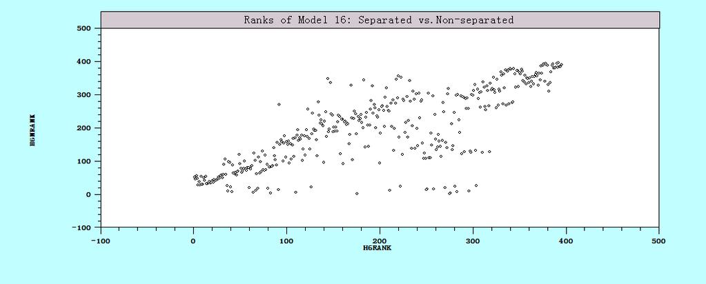
100 Figure 4.1 Rank correlation 87

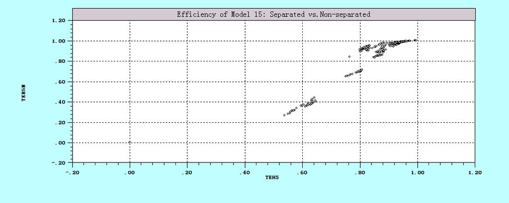
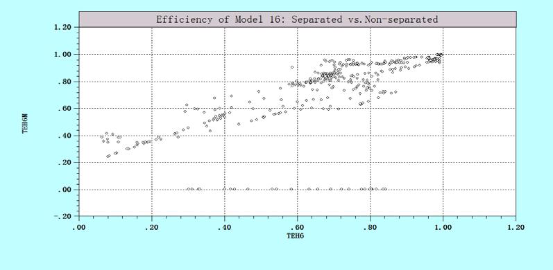
101 Figure 4.2 Efficiency correlation 88

102 Table 4.4 Correlation and rank correlation Model 14 Model 15 Model 16 Rank Efficiency From the comparison above, we could conclude that, the separated form and nonseparated form of production function are significant different. Whether including the cross terms of exogenous variable in the function or not does influence both the parameter estimation and technical efficiency estimation. Although the influence on the technical efficiency is unpredictable, the more sensible and consistent estimates of parameters and the significance of cross terms of the exogenous variable indicate that the non-separated form should be used in the following research Two Inputs Models The production frontier with two inputs is first estimated. The estimated parameters of different models are presented in Table 4.5 and Table 4.6. Models with exogenous variables including in the function are specified as the non-separated form. The scaling model does not work here. The scaling model requires the equality restrictions on the mean and the standard deviation of the distribution, which is too strict in our sample. Model 1 is the original model with homogeneity and homoscedasticity. All the models in Table 4.5 do not include the heterogeneity in the shape of technology, in other words, only capital, labour and time are included in the regressors. All the models suggest that the parameters of capital and labour are significant and have the value between 0 and 1, as expected. The structures of production technology are quite similar in these models. But the positive squared terms in most of the models are presented, which is inconsistent with the economic theory. Obvious technical inefficiency appears in most of the models except Model 10 and Model 12. The technical change shows both significant positive and negative influence on the output. The share of arable land shows negative influence on the mean of 89

103 inefficiency and negative on the variance of inefficiency; the share of government expenditure plays a positive role on the mean of u it and a negative role on the variance of u it ; the trade openness shows the positive influence on the variance of v it. Other effects on the mean and variance of u it and variance of v it caused by the exogenous variables are complicated and unstable in those models. For example, the signs of the trade openness effects on the mean of u it are significant and positive in Model 4 and Model 10, but significant and negative in the Model 11 and Model

104 Table 4.5 Results without heterogeneity in function as regressors (without energy) Parameter Model 1 Model 3 Model 4 Model 6 Model 7 Model 8 Model 9 Model 10 Model 11 Model 12 Model 13 β (0.1171) (1.6194) * (0.0183) (0.0241) * (0.0123) * (0.0113) β * * * * * * (0.0269) (0.0831) (0.0271) (0.0280) (0.0344) (0.0272) β * * * * * * (0.0210) (0.0327) (0.0266) (0.0270) (0.0322) (0.0256) β * * * * (0.0761) (0.1393) (0.0353) (0.0935) (0.0856) (0.0853) β * * (0.0699) (0.1056) (0.0424) (0.0872) (0.0745) (0.0837) β * * * * (0.1375) (0.2644) (0.0753) (0.1797) (0.1598) (0.1680) θ * * * * (0.0020) (0.0036) (0.0011) (0.0009) (0.0009) (0.0009) δ * * (0.2350) (0.0014) (0.0036) δ * * (0.2837) (0.0209) (0.0627) δ * (0.1570) (0.0141) (0.0456) γ (0.0236) (0.0359) (4.2531) (0.1564) * (0.0038) * (0.0037) * (0.0044) * * * * * (0.0083) (0.0570) (0.0177) (0.0191) (0.0178) * (0.0082) * (0.1028) * (0.0194) * (0.0205) * * * (0.0299) (0.0711) (0.0593) (0.0626) * * * (0.0284) (0.1070) (0.0562) (0.0582) * * * (0.0575) (0.1753) (0.1149) (0.1202) * * * (0.0002) (0.0128) (0.0007) (0.0007) * * (0.0122) (0.0121) * * (0.0273) (0.1219) * * (0.0155) (0.0420) * * (0.0433) (0.0492) (0.0555) * (0.0197) * (0.0728) * (0.0790) * (0.1504) * (0.0006) * (0.1204) * (0.2932) * (0.0472) * (0.0432) 91

105 Table 4.5 Results without heterogeneity in function as regressors (without energy) (Continued) Parameter Model 1 Model 3 Model 4 Model 6 Model 7 Model 8 Model 9 Model 10 Model 11 Model 12 Model 13 γ (0.2657) (0.2666) (4.0505) (0.4677) (0.1877) * (0.1645) * (1.1396) (0.4124) γ * (0.1216) (0.1827) (1.5362) * (0.1888) (0.1348) (0.1420) * (0.7845) (0.2476) η * (0.1407) * (0.1424) * (0.1727) η * * * (0.2812) (0.2650) (0.2823) η * (0.1055) * (0.0947) * (0.1116) μ * λ σ σ u σ v

106 The models in Table 4.6 incorporate the heterogeneity into the shape of production technology. Three exogenous variables are introduced into the function as regressors. Model 2 is the Pitt and Lee model with the three exogenous variables in the function form, but it does not work well here. The three models also give the similar estimates of the exogenous variables. All the three heteroscedasticity-adjusted models present the significant and negative effects of arable land and the share of government expenditure. The effect of trade openness is significant and positive. The negative effects of arable land are consistent with the world development trend. In modern world, the importance of urbanization for economic development is emphasized more and more, but the high urbanization and industrialization decrease the agriculture investment in both labour and capital. The result supports the importance of the industrialization hypothesis. As discussed above, there is a trade-off between the government investment and private investment, and the private investment is always more effective than the government expenditure, the higher share of government expenditure negatively affects the output. The positive sign of the trade openness indicates the importance of globalization in the modern world. Unlike the models in Table 4.5, where the share of arable land, the share of government expenditure and trade openness are only introduced into the heterogeneity and heteroscedasticity of error terms, some of the models report insignificant technical inefficiency with λ close to 0, such as model 10 and model 12. When the three exogenous variables are also introduced into the function form in Table 4.6, the technical inefficiency is present in all the models, with λ obviously different from 0. 93

107 Table 4.6 With heterogeneity in the function as regressors Parameter Model 14 Model 15 Model 16 β 0 β 1 β 2 β 11 β 22 θ α 1 α 2 α 3 δ 1 δ 2 δ 3 γ 1 γ 2 γ 3 η 1 η 2 η * (0.0148) * (0.0101) * (0.0098) * * * (0.0233) (0.0246) (0.0241) * * * (0.0210) (0.0228) (0.0219) * * (0.0602) (0.0698) (0.0727) * * (0.0524) (0.0657) (0.072) (0.0012) (0.0011) (0.0012) * * * (0.0098) (0.0082) (0.0094) * * * (0.0627) (0.0191) (0.0246) * * * (0.0308) (0.0194) (0.0198) (0.0055) (0.1184) * * (0.1088) (0.4072) * (0.0432) (0.0977) * (0.0664) (0.0911) * (0.3340) (0.7445) * * (0.1184) (0.1212) * (0.0940) (0.0463) (0.1036) * (0.3395) (0.5568) (0.5435) * * (0.1495) (0.2281) (0.2439) μ λ σ σ u σ v

108 Note: β1 is the parameter of capital, β 2 is the parameter of labour, α 1 is the parameter of arable land, α 2 is the parameter of government expenditure and α 3 is the parameter of trade openness. The measure of returns to scale is E = lny lnx i i (4.12) where both y and x i are mean corrected. When the return to scale is evaluated at the sample mean, it is the sum of the parameters of all the inputs. The estimates of returns to scale at sample mean for these models are shown in Table 4.7. Except Model 9 and Model 10, the models without heterogeneity in the function form all present the relative constant return to scale as we expected, with the estimates of return to scale at the sample mean close to 1. Model 9 and Model 10 are true random effects model. When the exogenous variables enter to the function form, the return to scale is slightly greater than 1, which is can be explained as the shifts from the three exogenous variables. Table 4.7 Returns to scale Model 1 Model 3 Model 4 Model 6 Model 7 Model 8 Model 9 RTS Model 10 Model 11 Model 12 Model 13 Model 14 Model 15 Model 16 RTS The next step is to analyze how the position of exogenous variables affects the technical inefficiency. The exogenous variables can be placed in the function form, the mean of u it, the variance of u it and the variance of v it, thus we have four groups plus one comparison between true fixed effects model and true random effects model to discuss. Group 1 Heterogeneity into function form We first investigate the effects when the heterogeneity is introduced into the function form. Three pairs are compared in Table 4.8, Model 11 and Model 14, Model 12 and Model 15, Model 13 and Model 16. Although most of the coefficients of exogenous variables are significant, as shown in Table 4.8, the introduction of them into the function form changes the estimates of inputs relatively little. In other words, adding exogenous variable shifts the production function only little, which is consistent with 95

109 the conclusion made by Greene (2007). The share of σ u in σ gets larger from Model 11 to Model 14 and from Model 12 to Model 15, while only a small decrease from Model 13 to Model 16. It can be explained as when more variables are introduced into the function form, less variation is left to be included into the error terms. When the exogenous variables are selected correctly, λ would be smaller. Table 4.8 Comparison (heterogeneity in the function form) Parameter Model 11 Model 14 Model 12 Model 15 Model 13 Model 16 β * (0.0038) * (0.0148) * (0.0037) * (0.0101) * (0.0044) * (0.0098) β * (0.0177) * (0.0233) * (0.0191) * (0.0246) * (0.0178) * (0.0241) β * (0.0194) * (0.0210) * (0.0205) * (0.0228) * (0.0197) * (0.0219) β * (0.0593) (0.0602) * (0.0626) * (0.0698) * (0.0728) * (0.0727) β * (0.0562) (0.0524) * (0.0582) * (0.0657) * (0.0790) * (0.072) θ * (0.0007) (0.0012) * (0.0007) (0.0011) * (0.0006) (0.0012) λ σ σ u σ v Figure 4.3 shows the kernel density estimates for the estimates of u i. The changes of the distribution of u i is unpredictable as in the estimates of σ u. When the heterogeneity are introduced into the function, the distribution of u i in Models 14 is looser in Models 14 than in Model 11, tighter in Model 16 than in Model 13, and there is no obvious change from Model 12 to Model

110 Figure 4.3 Kernel Density (heterogeneity in function form) Model 11 vs. Model 14 Model 12 vs. Model 15 Model 13 vs. Model 15 Table 4.9 displays the ranks correlation and simple correlation of technical efficiency between the three pairs of models. Both the ranks correlation and simple correlation indicate that the function forms with exogenous variables and without these exogenous variables tell different stories, even with the negative correlation around between Model 11 and Model 14. The scatter plots in Figure 4.4 also show the same results. The figures on the left are the correlation of efficiency and the figures on the right are the rank correlation. 97

111 Table 4.9 Correlation (heterogeneity in the function form) Model 11 vs. Model 14 Model 12 vs. Model 15 Model 13 vs. Model 16 Rank Efficiency Figure 4.4 scatter plots of ranks and efficiency (heterogeneity in function form) Model 11 vs. Model 14 Model 12 vs. Model Model 13 vs. Model 16 98

112 From all the analysis above, we could see that when the exogenous variables are directly introduced into the function, the influence on the function itself, like the estimates of capital and labour, is quite small, but it influences the technical inefficiency seriously and unpredictably. Group 2 Heterogeneity in the mean of u There are 6 pairs in this group, which are Model 1 and Model 3, Model 6 and Model 4, Model 7 and Model 8, Model 9 and Model 10, Model and 12 and Model 13, Model 15 and Model16. The only difference between the models in each pair is that the exogenous variables are introduced into the mean of u in the latter model, but not in the former one. Table 4.10 gives the main parameter estimation of these models. The change of estimated parameters of inputs is quite small in most of the models, except the true random effects pair, Model 9 and 10, which also show poor constant return to scale. The share of σ u in σ gets smaller in most of the models, except two pairs: Model 6 and Model 4, Model 12 and Model 13. Figure 4.5 shows the kernel density estimates for the estimates of u it. The changes of the distribution of u it are consistent in these models. The distribution of u it is looser when the exogenous variables are introduced into the mean of u it, Although the change is obvious in some models, like Model 9 and Model 10, Model 12 and Model 13, or slight in some models, like Model 1 and Model 3. Another visible distribution change is that the kurtosis of the density is much lower in the models with exogenous variable introduced into the mean of u it. The lower kurtosis indicates less of variance is the result of infrequent extreme deviations. 99

113 Table 4.10 Comparison (Heterogeneity in the mean of u ) Parameter Model 1 Model 3 Model 6 Model 4 Model 7 Model 8 Model 9 Model 10 Model 12 Model 13 Model 15 Model 16 β (0.1171) (1.6194) (0.0241) * (0.0183) * (0.0123) * (0.0113) β * * * * * * (0.0269) (0.0831) (0.0280) (0.0271) (0.0344) (0.0272) β * * * * * * (0.0210) (0.0327) (0.0270) (0.0266) (0.0322) (0.0256) β * * * * (0.0761) (0.1393) (0.0935) (0.0353) (0.0856) (0.0853) β * * (0.0699) (0.1056) (0.0872) (0.0424) (0.0745) (0.0837) θ * * * * (0.0020) (0.0036) (0.0009) (0.0011) (0.0009) (0.0009) * * * * (0.0037) (0.0044) (0.0101) (0.0098) * * * * * * (0.0083) (0.0570) (0.0191) (0.0178) (0.0246) (0.0241) * (0.0082) * (0.1028) * (0.0205) * (0.0197) * * * (0.0299) (0.0711) (0.0626) (0.0728) * * * (0.0284) (0.1070) (0.0582) (0.0790) * * * (0.0002) (0.0128) (0.0007) (0.0006) * (0.0228) * (0.0219) * * (0.0698) (0.0727) * * (0.0657) (0.072) (0.0011) (0.0012) λ σ σ u σ v

114 Figure 4.5 Kernel Density (heterogeneity in the mean of u ) Model 1 vs. Model 3 Model 6 vs. Model 4 Model 7 vs. Model 8 Model 9 vs. Model 10 Model 12 vs. Model 13 Model 15 vs. Model

115 Table 4.11 displays the ranks correlation and simple correlation of technical efficiency between the three pairs of models. Except Model 15 and Model 16 with the rank correlation 0.9 and simple correlation 0.8, none of these models show an obvious correlation. When the exogenous variables enter the mean of u it, the estimation of efficiency changes a lot, not only in the score, but also in the rank. Figure 4.6 displays the plots of the ranks and efficiency. Table 4.11 Correlation (heterogeneity in the mean of) 1 vs. 3 6 vs.4 7 vs. 8 9 vs vs vs.16 Rank Efficiency Figure 4.6 Scatter plots of ranks efficiency (heterogeneity in the mean of u) Model 1 vs. Model 3 Model 6 vs. Model 4 102

116 Model 7 vs. Model 8 Model 9 vs. Model 10 Model 12 vs. Model 13 Model 15 vs. Model

117 The estimation of parameters of inputs are quite stable when the exogenous variables are introduced into the mean of u it. The effect on the distribution of u it is consistent, while the influence on the efficiency is unpredictable. Group 3 Heteroscedasticity in u it All the models in this group compare the influence from introducing these exogenous variables into the variance of u it, σ 2 u. Four pairs are investigated here, which are Model 1 and Model 6, Model 3 and Model 4, Model 11 and Model 13, Model 14 and Model 16. From the Table 4.12, we could see estimates of inputs parameters change a lot in Model 1 and Model 6, Model 3 and Model 4 and is stable in the Model 11 and Model 13, Model 14 and Model 16. The latter two pairs include the exogenous variables in the variance of v it as well. 104

118 Table 4.12 Comparison (heteroscedasticity in u it ) Parameter Model 1 Model 6 Model 3 Model 4 Model 11 Model 13 Model 14 Model 16 β (0.1171) (0.0241) (1.6194) * (0.0183) * (0.0038) * (0.0044) * (0.0148) * (0.0098) β * (0.0269) * (0.0280) * (0.0831) * (0.0271) * (0.0177) * (0.0178) * (0.0233) * (0.0241) β * (0.0210) * (0.0270) * (0.0327) * (0.0266) * (0.0194) * (0.0197) * (0.0210) * (0.0219) β (0.0761) * (0.0935) (0.1393) * (0.0353) * (0.0593) * (0.0728) (0.0602) * (0.0727) β (0.0699) * (0.0872) (0.1056) (0.0424) * (0.0562) * (0.0790) (0.0524) * (0.072) θ (0.0020) * (0.0009) (0.0036) * (0.0011) * (0.0007) * (0.0006) (0.0012) (0.0012) λ σ σ u σ v

119 The kernel density is plotted in the Figure 4.7. But the influence on the distribution of u it is unstable, and no explanation for it is obvious. Some of them are becoming tighter when there is heteroscedasticity in the variance of u it, like the Model 14 and Model 16. Some of them are becoming looser, like Model 11 and Model 13. Figure 4.7 Kernel Density (heteroscedasticity in u it ) Model 1 vs. Model 6 Model 3 vs. Model 4 Model 11 vs. Model 13 Model 14 vs. Model 16 When the effect on the efficiency is detected, the same comparisons are applied as in the last two groups. Table 4.13 shows the poor correlation in both rank and technical efficiency. Figure 4.8 is the plot of rank and technical efficiency of the four pairs. 106

120 Table 4.13 Correlation (heteroscedasticity in u it ) 1 vs. 6 3 vs vs vs. 16 Rank Efficiency Figure 4.8 Scatter plots of ranks and efficiency (heteroscedasticity in u it ) Model 1 vs. Model 6 Model 3 vs. Model 4 Model 11 vs. Model

121 Model 14 vs. Model 16 Unlike the last two groups, where the estimation of parameters is stable, when the exogenous variables are introduced into the variance of u it, σ 2 uit, both the estimation of inputs parameters, the distribution of u i and the technical efficiency scores are changed unpredictably. Group 4 Heteroscedasticity in v it In this group, we compare the models with and without the heteroscedasticity in the random error term v it. Three pairs are detected here, which are Model 3 and Model 11, Model 4 and Model 13, Model 6 and Model 12. As shown in the Table 4.14, the differences in the estimation of inputs parameters in each pairs are relative tiny, except the parameters of capital in Model 4 and Model 13. The changes of σ u is not consistent, which decrease in the first pair and last pair, while increase in the second pair. 108

122 Table 4.14 Comparison (Heteroscedasticity in v it ) Parameter Model 3 Model 11 Model 4 Model 13 Model 6 Model 12 β (1.6194) * (0.0038) * (0.0183) * (0.0044) (0.0241) * (0.0037) β * (0.0831) * (0.0177) * (0.0271) * (0.0178) * (0.0280) * (0.0191) β * (0.0327) * (0.0194) * (0.0266) * (0.0197) * (0.0270) * (0.0205) β (0.1393) * (0.0593) * (0.0353) * (0.0728) * (0.0935) * (0.0626) β (0.1056) * (0.0562) (0.0424) * (0.0790) * (0.0872) * (0.0582) θ (0.0036) * (0.0007) * (0.0011) * (0.0006) * (0.0009) * (0.0007) λ σ σ u σ v The detection of kernel density is plotted in the Figure 4.9. No visible trend could be concluded from the three pairs. Figure 4.9 Kernel density (Heteroscedasticity in v it ) Model 3 vs. Model 11 Model 4 vs. Model

123 Model 6 vs. Model 12 The rank correlation and simple correlation of the technical efficiency are shown in the Table The first two pairs reveal a relative strong positive correlation in both rank and technical efficiency, around 0.7, while the negative correlation is very poor in the last pair. Scatter plots are shown in Figure 4.10 Table 4.15 Correlation (Heteroscedasticity in v it ). 3 vs vs.13 6 vs. 12 Rank Efficiency Figure 4.10 Scatter plots of ranks and efficiency (Heteroscedasticity in v it ) Model 3 vs. Model

124 Model 4 vs. Model 13 Model 6 vs. Model 12 Group 5 True Fixed Model vs. True Random Model True fixed effects models and true random effects models, which are important theoretical re-specification introduced in a series of papers by William Greene, e.g. Greene (2005), are compared in Table 4.16, where Model 7 and Model 8 are true fixed effects model, and Model 9 and Model 10 are random effects model. They are compared as two pairs: Model 7 and Model 9, Model 8 and Model 10. The estimates of parameters are significant different in the two model forms, and we have discussed that, the true random effects model does not report the reasonable estimation of inputs parameters. The share of σ u in σ gets lower when the model shifts from the true fixed effects to the true random effects, which is consistent with the property of the true random effects model, since it allows time invariant firm specific attributes to enter the model. The kernel density is shown in Figure

125 Table 4.16 Comparison (True FE vs. True RE) Parameter Model 7 Model 9 Model 8 Model 10 β * (0.0123) * (0.0113) β * (0.0344) * (0.0083) * (0.0272) * (0.0570) β * (0.0322) * (0.0082) * (0.0256) * (0.1028) β * (0.0856) * (0.0299) * (0.0853) (0.0711) β * (0.0745) * (0.0284) (0.0837) (0.1070) θ * (0.0009) * (0.0002) * (0.0009) (0.0128) λ σ σ u σ v Figure 4.11 Kernel Density (True FE vs. True RE ) Model 7 vs. Model 9 Model 8 vs. Model 10 The rank correlation and simple correlation of the technical efficiency are shown in the Table 4.17 and are plotted in the Figure With different assumptions of the 112

126 position of the exogenous variables, the correlation of true fixed effects model and the true random effects model go in opposite directions. When the exogenous variable only enter the variance of u it, the two models are positively correlated, while when the exogenous variables enter the mean of u it as well, the correlation of the two models is negative. It is difficult to frame a prior of these two models, but it reveals that position of exogenous variables affects the estimate of inefficiency strongly. Table 4.17 Correlation (True FE vs. True RE) 7 vs. 9 8 vs. 10 Rank Efficiency Figure 4.12 Scatter plots of ranks and efficiency (True FE vs. True RE) Model 7 vs. Model 9 Model 8 vs. Model

127 4.5.3 Three Inputs Models The results include energy as the third input are shown in Table 4.6 and Table 4.7. The signs and values of labour and capital are presented as expectation in most of the models in 4.18, with β 1 around 0.35 and β 2 around 0.50, except Model 11. The estimation of β 3, which is the coefficient of energy, is consistent in most of models. None of these models reports the reasonable estimation of the square terms. All of them are positive and significant. The technology change shows a significant positive effect on the production in all of these models. Comparing the values of the input coefficients with these values in the models without energy, we could see that, the coefficient of capital is stable, but coefficient of labour is lowered by the extra input energy, which is probably caused by the substitutability between inputs. When more energy is provided, the demand for labour will be lower. In other words, to produce the same amount of output, more energy indicates less labour demand. All of these models give obvious technical inefficiency except the model 9, the true random effects model. The true FE model even does not work here. As discussed in the last chapter, these models are time variant and pick up the cross unit heterogeneity beside technical inefficiency, but these advantages are not that appropriate in the world GDP production analysis. The influence of the exogenous variables in the heteroscedasticity is not consistent in these models. 114

128 Table 4.18 Results without heterogeneity in function as regressors (with Energy) Parameter Model 1 Model 4 Model 6 Model 9 Model 11 Model 12 Model 13 β (0.2608) * (0.0075) * (0.0094) * (0.0063) * (0.0057) (0.0064) β * (0.0545) * (0.0232) * (0.0224) * (0.0120) * (0.0164) * (0.0163) * (0.0158) β * (0.1077) * (0.0308) * (0.0300) * (0.0122) * (0.0207) * (0.0203) * (0.0211) β (0.0576) * (0.0121) * (0.0121) * (0.0057) * (0.0094) * (0.0093) * (0.0095) β (0.2270) * (0.0601) * (0.0620) * (0.0334) * (0.0548) * (0.0552) * (0.0532) β (0.4203) * (0.0760) * (0.0811) * (0.0449) * (0.0714) * (0.0705) * (0.0653) β (0.0337) * (0.0259) * (0.0255) * (0.0116) * (0.0189) * (0.0183) * (0.0171) θ (0.0073) * (0.0005) * (0.0005) * (0.0004) * (0.0004) * (0.0004) * (0.0004) δ (0.3969) (0.5962) (0.6689) δ (0.8887) (1.7584) * (0.3079) δ (0.1458) (7.4195) * (0.0766) γ * (0.0982) (0.0244) * (0.1386) (0.0230) * (0.2359) γ (0.4342) (0.2393) * (1.6246) (0.2644) (0.9286) γ * (0.1012) (0.1018) * (0.7014) (0.1342) (0.3024) η (0.1015) (0.1143) (0.0386) η * (0.4436) * (0.4317) * (0.4016) η * (0.1816) * (0.1892) * (0.1413) λ σ σ u σ v

129 The models in Table 4.19 include the exogenous variables in the function form as extra inputs. The estimations of the coefficients of each input are significant, consistent and realistic. The estimates of square terms are still positive as in Table 4.6. It is not surprising to find that the coefficient of the index of technology change t is positive in all the three models. These three models also give the similar and obvious technical inefficiency signals, and the influence of the extra variables on the variance of both error terms are the same. Then influence on the mean of u varies in Model 14 and Model 16. The proportion of arable land has a negative influence on the shape of the frontier, positive influence on the variance of u and negative influence on the variance v. The negative sign of arable land means the more the arable lands are transformed to other types of land, the higher the production frontier would be, which is same as in the Table 4.5 without energy input included. The signs of variances indicate that the influence of the proportion of arable land on the technical inefficiency is negative, since λ = σ u σ v. In other words, the urbanization leads to the higher technical efficiency. The government expenditure has a negative influence on the shape of the frontier, negative influence on the variance of u and positive influence on the variance of v. The negative influence on the shape of the frontier gives the same result as in the Table 4.5. But the negative influence on the variance of u and positive influence on the variance of v indicate that the negative influence on the technical inefficiency, since the negative influence on the variance of u leads to less vary in technical inefficiency and positive influence on the variance of v leads to more vary in the technical inefficiency. In other words, the higher government expenditure leads to a higher technical efficiency. Thus the control of government expenditure is quite important. There is a trade-off between the production frontier and technical efficiency. It is possible that the government expenditure is acting as proxy variable for the public funding of research and development support for industry. The openness also gives the same estimates as models in Table 4.5 of the influence on the shape of frontier. Together with the positive influence on the variance of u and negative influence of the variance of v, the results suggest that the openness 116

130 play an positive role in both production frontier and technical efficiency. This is consistent with the economic trend in the modern economy. Table 4.19 Results with heterogeneity in function as regressors (with energy) Parameter Model 14 Model 15 Model 16 β 0 β 1 β 2 β 3 β 11 β 22 β 33 θ α 1 α 2 α * (0.0106) * (0.0097) * (0.0088) * * * (0.0195) (0.0179) (0.0178) * * * (0.0198) (0.0165) (0.0169) * * * (0.0098) (0.0094) (0.0094) * * * (0.0400) (0.0298) (0.0320) * * (0.0445) (0.0381) (0.0385) (00160) (0.0137) (0.0122) * * * (0.0009) (0.0008) (0.0008) * * * (0.0095) (0.0083) (0.0070) * * * (0.0222) (0.0176) (0.0187) * * * (0.0179) (0.0015) (0.0141) 117

131 Table 4.19 Results with heterogeneity in function as regressors (with energy) (Continued) Parameter Model 14 Model 15 Model 16 δ 1 δ 2 δ 3 γ 1 γ 2 γ 3 η 1 η 2 η (0.0229) (0.0241) (0.0814) (0.3437) * (0.0564) (0.1194) (0.0852) (0.1706) * (0.2922) (1.1325) * (0.1186) (0.3185) * * * (0.0690) (0.0545) (0.0457) * * * (1.1334) (0.9373) (0.8569) (0.6162) (0.4425) (0.4600) λ σ σ u σ v The returns to scale at the sample mean are summarized in Table All the values are similar to values in the model without extra input energy. Most of them represent the constant return to scale with RTS around 1. The RTS in Model 9 is relative poor, which is Model 9 is the true random effects model. All the results show that the true random effects model report very weak coefficients estimation of inputs, according to the economic theory. The last three RTS are slight over 1 since the exogenous variables are directly included in the function in these models. 118

132 Table 4.20 Returns to scale (with energy) Model 1 Model 4 Model 6 Model 9 Model 11 Model 12 Model 13 Model 14 Model 15 Model 16 RTS In Table 4.21, the technical efficiency measures calculated from all the models are listed. As we can predicate, since the extra variables enter different positions in the model, the scores will be different from different models, with smallest value 36.4 in Model 16 and largest value 100 in Model 6, Model 12, and Model 15. Two remarks can be made from the technical efficiency. First, the ranges of different models change a lot. In Model 16, the smallest one is 36.4 and the largest number is 98.9, while in the Model 9, it is from 77.9 to Second, the ranks are also different from models, giving totally different meanings. The different ranks of United States and Japan are obvious. In Model 12, Model 13, Model 15 and Model 16, United States is ranked as No.1, while in Model 4 it is No. 21, the last but one, and No. 19 in Model 11. Japan is No.8 in Model 6 and Model 12, but the last one in Model 4 and Model 16. At this point, it is hard to say which model reports the perfect or right results. 119

133 Table 4.21 Technical efficiency (average scores over the period ) Country Model 1 Model 2 Model 3 Model 4 Model 6 Model 9 Model 10 Model 11 Model 12 Model 13 Model 14 Model 15 Model 16 Austria Belgium Denmark Finland France Greece Iceland Ireland Italy Luxembourg Netherlands Norway Portugal Spain Sweden Switzerland United Kingdom Australia New Zealand Canada United States Japan

134 4.6 Conclusion Unlike the homogeneity and homoscedasticity models in the last chapter, in this chapter the heterogeneity and the heteroscedasticity are introduced into the stochastic frontier panel models, which are more precise in practice. The arable land, government expenditure and trade openness are selected as exogenous variables. The position of exogenous variables, the separated form and non-separated forms, the models with energy and without energy as input besides labour and capital are detected. We can find that it is hard to say which model performs better than the others. The form of production function, the position of extra variables, and the selection of inputs all affect both the shape of frontier and the technical efficiency. The most consistent and relative reasonable results are shown in Table 4.7, which contains the models with more regressors than other model, and with more positions where the exogenous variables located. But we cannot conclude that the more variables included, the better the model is. The score of technical efficiency varies sharply even in these models. From the discussion above, we could say that when the heterogeneity and heteroscedasticity are considered, the selection of stochastic frontier panel data models must be done very carefully, at least at the macroeconomic level, not only the position of the exogenous variables, but also the selection of the regressors and the function forms. Where to put the extra variables? is a question that is not answered yet. From the application to the world GDP analysis, we could find that when heterogeneity and heteroscedasticity are considered into the function, either into the shape of production technology or the error terms, the parameter estimation of two main inputs are quite similar. That is to say, the position of extra variables does not influence the parameters of main inputs obviously, but it does influence the technical efficiency in both the value and the rank. 121

135 Chapter 5 Models applied to Italian Manufacturing Industries 5.1 Introduction In the last two empirical chapters, all the stochastic frontier models are applied to the country level datasets, which are considered as on the macroeconomic level. In this chapter, the comparison of panel data stochastic frontier models is applied to a microeconomic level dataset. The production of Italian manufacturing is investigated. The main variables include output, labour and capital. Market share, sector, legal form, the behaviour of export, the age of firms and the location are selected as the exogenous variables. Cobb-Douglas function form and translog function form are compared and the translog function is applied. The models contain both classical models and new developed models, which are Pitt and Lee (1981), Schmidt and Sickles (1984), Battese and Coelli (1992, 1995), true fixed effects model, true random effects model, fixed management model and the latent class model. The models are applied to three categories: with heterogeneity and heteroscedasticity, with only heterogeneity in the function form, and with both heterogeneity in the function form and heteroscedasticity in the error, the results show that the classical models perform better than the newly developed models in both economic and statistical aspects. 122

136 The organization of this chapter is as follows. A brief overview of Italian manufacturing and the details of the dataset and variables are shown in section 2. Section 3 expresses the models, the results and the discussion of them. Conclusions are summarized in Section Italian Manufacturing An Overview of Italian Manufacturing Industry Italian manufacturing industries play an import role in the Italian economy. (World economic outlook database 2010) The largest business is engineering, followed by construction and textile. Most manufacturing companies are located in the north of the Italy, with very few large factories in southern Italy.( Mignone 2008) But in recent years, some firms relocated their operation sectors in the south of Italy, with the benefit of tax reduce and flexible workforce, although the southern parts are still poor. The major components of Italian manufacturing are small and medium sized companies, run by family, and only a few are large enterprises and state-owned. The major components of Italian manufacturing industries are light manufacturing industry, heavy manufacturing industry, and food processing industry. As the most import heavy manufacturing industry, the design and production of automobile and the machine parts of automotive vehicles are highly trusted in the worldwide, which are the largest contribution to Italy GDP and are a large portion of Italian export. It is also the largest business in Italy economy. The most famous company in automotive industry is FIAT (Fabbrica Italiana Automobili Torino), which owns the worldwide well known brands, like Alfa-Romeo, Lancia, and Ferrari. There is a idea saying what is good for FIAT is good for Italy to describe the high status of automotive industry in Italian government and economy. In the light manufacturing industry, the textile and clothing industry is most important, which is the third largest business in Italy economy. It is also well-known for the design and production with lots of famous brands, such as Armani, Valentino, Gianfranco, Versace and Krizia. The excellent design, high quality and relative inexpensive prices make the textile and clothing industry has a strong competition in 123

137 the world market and export to every corner of the world. The eye wear and leather goods are also the components of the light manufacturing industry. The food processing industry is built on the reputation and popularity of Italian traditional foods, such as cheese, pasta, sausage, chocolate and ham. Most of the food processing firms are small and medium sized, focusing on the local food supply, but they also have many well-known brands, such as Barilla, Parmalat, and Nestle, exporting to foreign markets Variables and Data Information The output is indicated by the deflated Net Sales as a single output. Two traditional inputs, labour and capital are indicated by total number of employees and net physical capital asset, separately. The expectations of labour input and capital input are the same as last chapter. Returns to scale will be detected. 6 exogenous variables are discussed, which are market share, location of the firm, export, legal form of the firm, age of the firm and sectors. The market share is measured by the proportion of the net sales of an individual firm to the net sales of the sector which the firm belongs to. Here, the sectors are separated by the Italian national classification Ateco 91, which is a five-digit classification according to the economic activities. The first three digits indicate the sector of the firm, and the last two digits indicate the further sub classification. The influence of market share is expected to be positive to the production of the firm. But as we discussed in the literature review chapter, when the firm is monopoly in the sector, their aim could be looking for the stable situation but not the maximum output. The map of Italy is long and narrow with three islands. Based on development level, Italy is considered to be a north-south division. The northern Italy is highlyindustrialized, while the southern Italy is less advanced and more based on agriculture and tourism. The northern Italy includes 12 regions in the northern and central area, which are Emilia-Romagna, Friuli, Lazio, Liguria, Lombardia, Marche, Piemonte, Toscaand na, Trentino-Alto Adige, Umbria, Valle D Aosta and Veneto. 124

138 The southern Italy includes the regions in the southern area and the islands, which are Abruzzo, Basilicata, Calabria, Campania, Molise, Puglia, Sardegna and Sicilia. In our research, the location of firm is a dummy variable, with northern Italy denoted as value one and southern Italy denoted as value zero The effect of location is investigated to see whether the firms in northern Italy perform better than the firms in southern Italy, which is expected to be positive influence on the production. Italy has the world s sixth highest exports, and the Italian manufacturing industry is export-oriented. The major exports are food, clothing, precision machinery, motor vehicles chemicals and electric goods. The export-oriented economy has its own advantages and disadvantages. On one hand, these economies export their competitive advantage products to the foreign markets, which could encourage the firms to be more professional and more efficient, and allocate the resources more rescannable. On the other hand, these firms are market sensitive to exogenous factor. Both exchange rate and financial crisis highly influence the export-oriented economy. The main export markets for Italy are European countries, and the uniform currency Euro may have negative influence on the Italian economy. Whether export activities could improve the production technology and reduce technical inefficiency will be detected This variable is a dummy variable, which takes value one when the firm has export activity and take value zero when the firm does not have the export activity. Since technological and market conditions can vary over sectors, the sectors are included as a dummy variable in our research. The sectors are classified by the Pavitt s taxonomy, which includes four classes of industrial firms: Sector 1: Supplier-Dominated: includes firms from mostly traditional manufacturing such as textiles and agriculture which rely on sources of innovation external to the firm. Sector 2: Scale-Intensive: characterized by mainly large firms producing basic materials and consumer durables, e.g. automotive sector. Sources of innovation may be both internal and external to the firm with a medium-level of appropriability. Sector 3: Specialized Suppliers: smaller, more specialized firms producing technology to be sold into other firms, e.g. specialized machinery production and 125

139 high-tech instruments. There is a high level of appropriability due to the tacit nature of the knowledge. Sector 4: Science-based: high-tech firms which rely on R&D from both in-house sources and university research, including industries such as pharmaceuticals and electronics. Firms in this sector develop new products or processes and have a high degree of appropriability from patents, secrecy, and tacit know-how. The four dummy variables take value one when the firm belongs to the corresponding sector; otherwise it takes value zero. The legal form also has important influence on the firm s production. On one hand, Public Limited Companies (PLC) are expected to be more efficient than other legal forms, because the commercial risk is limited to the share capital, so they can take higher risks with expected higher returns on their investment projects. One the other hand, since the owners and managers have different objectives, the principle-agent problem could decrease the firm s efficiency. The legal form is a dummy variable with value one if the firm is a PLC, otherwise with value zero. The legal form of the firms 1. Sole proprietorship 2. Partnerships (Society of fact, general partnership, limited partnership) 3. Capital companies (joint stock company, limited by shares, limited liability) (plc in UK) 4. Cooperative Society 5. Other legal form The age of a firm is also considered as an important exogenous variable. The older firms are considered more experienced and enjoy the benefit of learning, but these firms are always prone to inertia, and have the bureaucratic problems, thus they can not adjust to change as rapidly as the younger firms do. The older firms also suffer the higher labour costs than younger firms, which are caused by the onerous pension obligations. The age variable is measured as the number of years since the firm established to the year

140 All the data are drawn from a rich firm-level database, the survey Indagine Sulle Imprese Manifatturiere (ISIM), conducted by the Italian investment bank CAPITALIA. This survey is conducted every three years through the questionnaires response by managers and supplemented with the financial statements of those firms. The approximate 5000 firms selected in the survey are the Italian manufacturing firms within the national boarders and with more than ten employees. The data are categorized by geographical area, firm size (the number of employees), and industry sectors. Both qualitative and quantitative information are supplied by the survey, which cover a wide range of firm characteristics including labour force variables, the ownership, investment activities and finance. The data set used in this chapter is from the eighth wave of ISIM, conducted in 2001, which includes more than 4000 manufacturing firms from 1998 to From the original sample, a number of firms have been eliminated, due to the lack of relevant data. The firms going through the merger or division during 1998 to 2000 are not included in the sample. Thus, an unbalanced panel data with 4021 firms from 1998 to 2000 is used in this chapter. The summary statistics of the data are presented in Table 5.1. Table 5.1 Data information Variable Mean Std. Dev. Minimum Maximum Net Sales Labour Capital Market Share Age The Models and Results The organization of model comparison Because of the diversities of the stochastic frontier panel models, the comparison is run by the following four steps 127

141 Step 1: compare the Cobb-Douglas and Translog function form, using the Pitt and Lee model. Step 2: compare the 4 simplest models without Z variables included: Pitt and Lee, Schmidt and Sickles (1984), Cornwell, Schmidt and Sickles (1990), and Battese and Coelli (1992) Step 3: include the Z variables in the function form. Apply to BC(1992), Pitt and Lee, True FE and True RE, and Fixed Management model. Step 4: models with heteroscedasticity in the inefficiency component. Apply to BC(1995), Pitt and Lee, True FE, True RE, Fixed management, and latent class. The purpose of the comparison is to detect the appropriate properties of these models in both statistical structure and the economic sense. The distribution of u it, and v it, and the properties of estimators are investigated as the statistical aspect, while the signs of the parameters, the elasticity and return to scales are investigated as the economic aspect Cobb-Douglas function VS. Translog function Since our data set is a short panel with only 3 time periods, it is reasonable to suppose that the inefficiency is time invariant. The Pitt and Lee model is used to compare the two production function forms in this step: Cobb- Douglas function form and translog function form. The difference between them is that the former does not include the cross terms in the function, but the latter does. The model proposed by Pitt and Lee in 1981 is a time invariant, random effects model, written as y it = α + β x it + v it u i (5.1) The inefficient component is assumed to be time invariant, denoted subscript with i but not it. The normal-half normal distribution assumption is applied to the data set. The estimation results are shown in the Table

142 Table 5.2 Comparison of Cobb-Douglas function and translog function Cobb-Douglas Translog constant *** *** x *** *** x *** *** 2 x *** 2 x *** x 1 x *** x 1 t *** x 2 t 0.121** t *** *** t *** *** λ σ u σ v χ Note. *,**,*** significance from zero at 10%, 5%, 1% level. From Table 5.2, we could see that, when cross terms are included in the function, the estimation of the coefficient of labour does not change a lot, from 0.11 to 0.12, but the estimate of the coefficient of capital changes from 0.87 to 0.78, which indicates that the capital influence on production are more sensitive to these cross terms. All the estimates of cross term are significant with 5% significance in the translog form function, and the chi square test also shows the significant difference between these two function forms. Different from the estimates of coefficients, there is no obvious difference of technical inefficiency between these two function forms. When the ranks of technical efficiency are compared, a high correlation score is reported: The Figure 5.1 also shows the high correlation between the two ranks. Thus, it is summarized as although the cross terms affects the coefficients estimation, the technical inefficiency is not affected significantly. And obviously, when more regressors are included in a function, the coefficients would be changed. To make both the estimates of coefficients and the estimates of technical inefficiency are accurate, the translog production function form is applied in the following analysis. 129

143 Figure 5.1 The rank correlation of Cobb-Douglas function and translog function Models without heterogeneity and heteroscedasticity The comparison starts from the simplest situation, with no exogenous variables included. Four classic models are applied in this step. The model proposed by Pitt and Lee (1981), the model proposed by Schmidt and Sickles (1984), the model suggested by Cornwell, Schmidt and Sickles (1990), and the model suggested by Battese and Coelli (1992). The first two models are time invariant with i as the subscript. The last two models assume that the inefficiency term is a function of time t. Pitt and Lee (1981) s model is introduced in the last step. Another time invariant model is suggested by Schmidt and Sickles (1984), which is a fixed effects model. The model assumes that the technical inefficiency is time invariant and fixed to each firm. y it = α i + β x it + v it (5.2) where α i = α u i Unlike other models the most efficient firm in this model gets the inefficiency score as 0, since u i = max(α i ) α i. Thus we expected that the efficiency score obtaining from this model is higher than others for the firms, if they have the similar ranks. 130

144 To relax the time invariant assumption, Cornwell, Schmidt and Sickles (1990) proposes a quadratic function between α it and time. Unlike only one most efficiency firm in the Schmidt and Sickles model, the most efficiency firm could be changed from time to time with this specification. α it = θ i0 + θ i1 t + θ i2 t 2 (5.3) But the estimation procedure of the CSS model requires a large matrix with NT N, which is too large to run by the software since the number of individual firms in the sample is too large. Battese and Coelli (1992) suggests another form of the time varying model, the function of u it and time t is u it = g it U i = exp[ η(t T)] (5.4) The Pitt and Lee model actually is a special case of Battese and Coelli model, with g it = 1. The data set used here is a short panel, thus we expect these models report similar results about the inefficiency estimates. Since both the SS model and PL model are time invariant, to make the comparison, the inefficiencies in Battese and Coelli s model is taken the average value during the three-year time period. The CSS (1990) model does not work for this dataset, and the explanation is shown in the conclusion. All the estimate results are shown in Table 5.3. The coefficients estimation of labour and capital are economically reasonable in all the models, with around 0.1 for labour and around 0.7~0.8 for capital. But both the parameters from SS models are smaller than the others. The technical change gives the significant positive influence on the production, with positive parameters for t and t

145 Table 5.3 The estimation results SS BC(92) PL Constant *** *** x *** *** *** x *** *** *** 2 x *** *** 2 x *** *** *** x 1 x *** *** x 1 t * *** *** x 2 t ** ** ** t ** *** *** t ** *** *** λ *** *** σ u σ v Note. *,**,*** significance from zero at 10%, 5%, 1% level. The measure of returns to scale is E = lny lnx i i (5.5) where both y and x i are mean corrected. When the return to scale is evaluated at the sample mean, it is the sum of the first order parameters of all the inputs. The returns to scale at the sample mean are shown in Table 5.4. The returns to scale for BC model and PL model are similar and close to 1 as economic theory expected, but for SS model, it is only 0.87, far from 1. Table 5.4 Returns to Scale Model SS BC(92) PL RTS Table 5.5 The technical efficiency correlations between the four models SS PL(92) BC SS PL

146 BC(92) Table 5.6 Compare the rank between the four models SS BC(92) PL SS BC(92) PL As we expected before, the Battese and Coelli s model and Pitt and Lee s model give the similar coefficients estimation, the similar technical efficiency estimation, with a high correlation , and the similar rank estimation, with the rank correlation The Pitt and Lee model is the special case of Battese and Coelli (1992) model when it is time invariant. The time period is only three years in our dataset and the change in the technical inefficiency is slight year by year, thus the average score of technical inefficiency used to compare with the Pitt and Lee model should be similar to the time invariant technical inefficiency. It is not a surprise to see these two models give quite similar results in both coefficient estimation and technical estimation. The plot shows the same result. The SS model shows a different picture from the two models discussed above. Although the rank correlations indicate almost no difference of the rank estimations among these models, the coefficient estimates and the technical efficiency estimates are make this clearer, e.g. the estimates are very different from the other models. When the technical efficiency is detected in Table 5.7, the SS model s estimates are not that reasonable, since the gap between the most efficient firm and the most inefficient firm is too large, suggesting a dominant influence from outliers. In a competitive market, a firm with such a low efficiency is hard to survive. The extreme situation is caused by the model assumption and the estimation method. Since the result is not the absolute inefficiency, but inefficiency of a firm relative to the other firms in the sample, the rank of them should similar to the rank obtained from the absolute inefficiency estimates. The problem with this method is that it shifts the regressing line to obtain the frontier, by only changing the intercept. The frontier is parallel to the OLS regression line. The frontier itself does not reflect the 133

147 real potential output, thus the estimates are different from the other two models. The SS models could be treated as the linear regression models with fixed effects but not the frontier. Table 5.7 The statistic of technical inefficiency Mean Minimum Maximum SS PL BC(92) Figure 5.2 the rank correlations SS vs. BC (1992) SS vs. PL PL vs. BC (92) The kernel density of technical inefficiency terms of these models are shown in Figure 5.3. Although all of them are positive skewed, the technical inefficiency from SS model is significant different from the other two. Not only the mean, the minimum value and the maximum value, which are different because of the original 134

148 assumption and estimate method, but also the distribution. The distribution of technical inefficiency obtained from SS model is symmetrical, but the other two models are not. 135

149 Figure 5.3 The kernel density Battese and Coelli (1992) Pitt and Lee (1981) 136

150 Schmidt and Sickles (1984) From the comparison and analysis above, we could conclude that the Battese and Coelli (1992) model and the Pitt and Lee (1981) model are actually the same in a extremely short panel. Although the technical change gives positive influence on the production, the technical inefficiency is time invariant. The Schmidt and Sickles (1984) model is also time invariant, but its foundation is not the real frontier, which should be the maximum output at a given input level, as shown in Figure 5.4. The straight line is the frontier obtained from SS model and curve is real frontier. At the input level x 0, the real maximum output should be on the point A with output y 0. If the SS model is applied, the maximum output is on the point B with output y 1, which is greater than the real maximum level, thus the technical inefficiency would be higher than the true technical inefficiency. The SS model simplifies the estimation, by only shifting the OLS regression line parallelly, and an inappropriate frontier is used, which leads to the inappropriate estimation of both coefficient estimation and technical estimation. The SS model is not suggested in the frontier analysis. 137

151 Figure 5.4 The problem with SS (1984) y SS y 1 y 0 B A Real frontier x 0 x No exogenous variables are included in the models in step 2. In the following two steps, 6 exogenous variables are included in the model as additional regressors and the heteroscedastic terms. Not only the classic models, but also some new models developed recent years are compared Models with heterogeneity The market share, section, location, legal form, firm age, and export are introduced into the function as regressors in this step. Data set is applied to Battese and Coelli(1992), Pitt and Lee (1981), True Fixed Effects model and True RE model, Fixed Management model. The exogenous variables are introduced into the function form as extra regressors in this part. Although the function form is translog function, these extra regressors are introduced as separated form, that is, no cross terms of these extra variables. How many regressors should be included in the function form is always a problem, not the more the better. If there are too many regressors in the function, the estimation of the most important regressors would be imprecise, since the estimation of other 138

152 unnecessary regressors reduce the efficiency of coefficients estimation. The separated translog function is written as y it = α i + K k=1 β k,i x it,k K M + γ km x it,k x it,m + η h.i z it,h + v it u it k=1 m=1 where z it is the exogenous variables. The Battese and Coelli s model (1992), Pitt and Lee s model, the true fixed and true random models are applied here. In these exogenous variables, most of them time invariant dummy variables, such as the location, the legal form, the export and the sectors. Only market share and age are time varying variables. But since the two variables would not change too much for most of the company in three years, the results obtained from time invariant models and time varying models are expected to be similar. Some information could be found from the data directly, like the change of market share in different sectors. The market share of firms in the Sector 1 do not change too much in the three years, and most of them are more than 20 years old firms, only quite a few are less than 10 years. This is because the first sector is classified as the traditional manufacturing, such as agriculture and textile. These manufacturings rely on the resource supply more than the technique. And the experience of management, the reputation built up year by year and the stable supply-demand relations are more important for the firm in this sector, which are the advantages owned by older firms. In other words, the new companies do not have obvious advantages in sector one, and it is not easy to enter. On the other hand, the market share of firms in the fourth sector, the science-based sector, changes more obviously than in the first sector and more young firms are found in this sector. The technical revolution plays an important role in these high-tech firms, and the entry barrier is relatively low in this sector. True Fixed Effects Model and True Random Effects are first proposed by William Greene (2004, 2005). The main argument is that the inefficiency component in the traditional fixed effects model or random effects model absorbs the cross firm H h=1 139

153 heterogeneity which should be presented as regressors in the function but not as inefficiency. Thus he suggested the true fixed effects model, expressed as y it = α i + β x it + v it u it (5.6) where α i is the firm specific intercept intended to capture all the time-invariant hetergeneities. The true random effects model is written as y it = α + β x it + v it u it + ω i (5.7) where ω i is a time invariant firm specific random term intended to capture cross firm time invariant heterogeneity The fixed management model is proposed by Alvarez, Arias and Greene (2006). An unobservable, time invariant variable is introduced into the model, labelled management in their paper. The core function is y it = f(x it,1, x it,2,, x it,k, m i ) (5.8) This model is actually a random parameters model with random constant term and first order terms, and non-random second order terms in a translog model. All the parameters are the function of the same single random effect, w i, which is time invariant and normally distributed with variance 1. K K M y it = α i + β k,i x it,k + γ km x it,k x it,m + v it u it k=1 k=1 m=1 α i = α + θ α w i + θ αα ( 1 2 w i 2 ) β k,i = β k + λ k w i w i ~ N[0.1] v it ~ N[0, σ 2 v ] u it ~ N[0, σ 2 u ] (5.9) The basic idea of latent class model is that there is unobserved heterogeneity in the distribution of y it, and that this heterogeneity is assumed to influence the density in a 140

154 random effect form. The distribution of this heterogeneity is continuous, but it is estimated approximately by estimating the location of a finite number of points of support and the probability within each interval. These intervals are defined as class, which are unknown, time invariant, and the number of points of support is chosen by the analyst according to the empirical condition. y it j = β j x it + v it u it v i j = N[0, σ 2 vj ] u i j = N[0, σ 2 uj ] (5.10) where j indicates the unknow classes, the firms in each class have the same coefficienct estimates, and the error terms are time invariant in each class. The results of these models are shown in Table 5.8. In order to make the comparison, the estimation in the latent class model are the weighted average value from the three classes. The details of each class are discussed later. 141

155 Table 5.8 The results of models with heterogeneity Pitt and Lee BC(92) FM Latent Class Constant *** *** *** x *** *** *** x *** *** *** x *** *** *** x *** *** *** x 1 x *** *** *** x 1 t *** *** * x 2 t *** *** ** t *** *** *** t *** *** *** Market share *** *** *** Sector *** *** *** Sector *** Sector *** *** *** Legal form *** Export *** *** *** Location *** *** *** Age *** *** * λ *** *** *** σ u σ v Note: 1. the coefficients on constant, x1, and x2 in the fixed management model are the mean of the random parameters. 2. The coefficients in the latent class model are the weighted average value of all the classes. 3. *,**,*** indicate the significance from zero at 10%, 5%, 1% level. Table 5.9 Returns to Scale Model Pitt & Lee BC(92) FM Latent Class RTS

156 Table 5.8 reports that the Pitt and Lee model and Battese and Coelli (1992) model give the similar estimation in both coefficients estimation and technical inefficiency estimation as before even more regressors are included. This is a further proof of the uniform of PL model and BC(1992) model in an extremely short panel. Both the parameter estimation of labour and capital are lower than the model without exogenous variables. The decrease is caused by the more regressors introduced into the function with positive influence on the production. The effects from technical change do not change too much comparing with the models without exogenous variables. The market share plays a significant positive role on the production in the two models as expected, with a high value The legal form of a firm has insignificant influence on the production. The significant positive parameter of export indicates that the firms with export activities produce more products than the firms without export activities. As we expected, the firms located in the northern Italy producer more. The effects from the age of firm is small but significant, which indicates that although the younger firms have the quicker reflection to the external environment, the experience, the mature management and other advantages taken by the older firms are more important to the firm s production. The influence from the sectors is expected to be significant, but the results show the insignificant effects from sector 2, which captures the mainly large firms in the manufacturing. It is probably because the number of firms in this sector stays relatively constant and is relatively small, therefore it accounts for a low share of the variability in the dependent variable. The significant technical inefficiency is confirmed by the nonzero λ. The returns to scale in PL model and BC(92) model are smaller than the returns to scale in the models without exogenous variables. The results is caused by the more variables are introduced into the function form. The coefficient estimation from fixed management model are different from PL model and BC(1992) model. The parameter of labour is greater while the parameter of capital is smaller, but the returns to scale does not change too much. The fixed management model also reports different effects from the exogenous variables. The market share still has significant positive parameter but smaller than PL and BC, from 0.93 to The influence from sector 1 does not change, but sector 2 now gives significant influence unlike insignificant influence in PL and BC. The sign of 143

157 parameter of sector 3 is even reversed. The parameter of legal form is significant here unlike in the other two models. The export shows the greater effects in the fixed effects model. While the age of firms is only significant at the 90% significant level and it is negative. A significant technical inefficiency is reported by the fixed management model. Since the absolute efficiency score in different models may vary a lot. It is more reasonable to compare the rank of efficiency in different models. The rank correlations are shown in Table 5.10, and the plot of the ranks are shown in Figure 5.5. Table 5.10 Rank correlations PL BC(92) FM PL BC FM Figure 5.5 The plots of rank correlation PL vs. FM 144

158 BC (92) vs. FM PL vs. BC (92) As expected, the rank correlation of PL and BC(92) are high and close to 1. The rank correlations between PL and FM and between BC and FM are only around But the plots show that most of the points are centralized in the area between the bold lines. The latent class model is first fitted with no specification of the influence in the prior probability, and then fitted with specifying the location, age, sector, legal form and 145