Dr Ian R. Manchester Dr Ian R. Manchester AMME 3500 : Root Locus

Transcription

1

2 Week Content Notes 1 Introduction 2 Frequency Domain Modelling 3 Transient Performance and the s-plane 4 Block Diagrams 5 Feedback System Characteristics Assign 1 Due 6 Root Locus 7 Root Locus 2 Assign 2 Due 8 Bode Plots 9 Bode Plots 2 10 State Space Modeling Assign 3 Due 11 State Space Design Techniques 12 Advanced Control Topics 13 Review Assign 4 Due Dr. Ian R. Manchester Amme 3500 : Introduction Slide 2

3 System 1 (e.g. Controller) System 2 (e.g. Process) System 1 affects system 2, which affects system 1, which affects system 2. Slide 3

4 Vehicle Control and Design (land, sea, air, space) understanding and controlling how the system responds to external disturbances Biomedical (cardiac system, dialysis machine) design and control of systems that interact with the human body. Manufacturing Processes controlled conditions for highperformance materials, pharmaceuticals, microsystems. Biological feedback systems that regulate pressures, concentrations, balance, etc Slide 4

5 Design the dynamics Sluggish systems become quick to respond Unstable systems become stable and predictable Robustness Reject disturbances acting on the system Same response with large variations in the system Slide 5

6 Pole location of a linear time-invariant system determines many important system properties such as: Stability, settling time, overshoot, rise time, oscillation. Slide 6

7 Feedback is important because of the ability to stabilize unstable systems, react to disturbances, and reduce sensitivity to changing system properties. But how does feedback affect system properties? I.e. what happens to pole locations under feedback? Slide 7

8 Slide 8

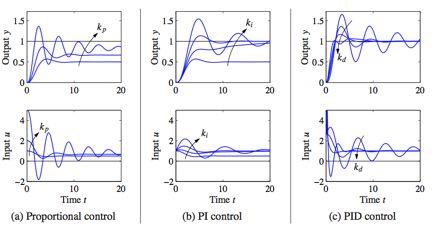
9 Same torsional setup as before P control: K=100 PD control: K(s)=100+10s PID control: K(s)=80+60/s+6s Note the zero steady-state error for PID Slide 9

10 PID with Different spring constants: k =5 (nominal), 7.5, and 2.5 Nm/rad Slide 10

11 r(t) G d G n d(t) Slide 11

12 For the moment let us examine a proportional controller. (Other control structures such as integral and derivative terms may be lumped in to G(s)). R(s) E(s) C(s) + - K G(s) Slide 12

13 Closed-loop transfer function is: T(s) = KG(s) 1+ KG(s) For example, if G(s) = 1 (s + a)(s + b) Then T(s) = K s 2 + (a + b)s + ab + k Slide 13

14 We could compute the system parameters as a (highly nonlinear) function of the gain, K Then for each possible K, computer system parameters and try to find one that fits. Trial and error is not a good design principle! Slide 14

15 In 1948 Walter Evans invented a technique for analysis of feedback systems while working as a summer intern at North American Aviation (now Rockwell International). It gives surprisingly simple rules for how pole locations change when feedback gain is adjusted Despite the huge changes in computational power since then, it is so intuitive and useful that it is still widely used for design and analysis Slide 15

16 Consider a simple control system: tilt control on a camera. Open loop poles are at zero and -10. How can we choose a feedback gain to give some desired performance? Slide 16

17 We could determine the closed loop poles as a function of the gain for the system Slide 17

18 The individual pole locations The root locus Slide 18

19 Remember our description of system specs as a function of pole location. So by increasing gain we can reduce settling time up to a point, beyond that we will induce large overshoot. The system always remains stable! n (decreasing T r ) Slide 19

20 We can easily derive the root locus for a second order system What about for a general, possibly higher order, control system? Poles exist when the characteristic equation (denominator) is zero Slide 20

21 How do we find values of s and K that satisfy the characteristic equation? This holds when Slide 21

22 Rule 1 : Number of Branches the n branches of the root locus start at the poles For K=0, this suggests that the denominator must be zero (equivalent to the poles of the OL TF) The number of branches in the root locus therefore equals the number of open loop poles Slide 22

23 Rule 2 : Symmetry - The root locus is symmetrical about the real axis. This is a result of the fact that complex poles will always occur in conjugate pairs. (otherwise coefficients of the system s differential equations would be complex, which is not physical) Slide 23

24 Rule 3 Real Axis Segments According to the angle criteria, points on the root locus will yield an angle of (2k+1)180 o. On the real axis, angles from complex poles and zeros are cancelled. Poles and zeros to the left have an angle of 0 o. This implies that roots will lie to the left of an odd number of real-axis, finite open-loop poles and/or finite open-loop zeros. Slide 24

25 Rule 4 Starting and Ending Points As we saw, the root locus will start at the open loop poles The root locus will approach the open loop zeros as K approaches! Since there are likely to be less zeros than poles, some branches may approach! Slide 25

26 Consider the system at right The closed loop transfer function for this system is given by Difficult to evaluate the root location as a function of K Slide 26

27 Open loop poles and zeros First plot the OL poles and zeros in the s-plane This provides us with the likely starting (poles) and ending (zeros) points for the root locus Slide 27

28 Real axis segments Along the real axis, the root locus is to the left of an odd number of poles and zeros Slide 28

29 Starting and end points The root locus will start from the OL poles and approach the OL zeros as K approaches infinity Even with a rough sketch, we can determine what the root locus will look like Slide 29

30 Rule 5 Behaviour at infinity For large s and K, n-m of the loci are asymptotic to straight lines in the s-plane The equations of the asymptotes are given by the real-axis intercept, " a, and angle, # a Where k = 0, ±1, ±2, and the angle is given in radians relative to the positive real axis Slide 30

31 Why does this hold? We can write the characteristic equation as This can be approximated by For large s, this is the equation for a system with n-m poles clustered at s=" Slide 31

32 Here we have four OL poles and one OL zero We would therefore expect n-m = 3 distinct asymptotes in the root locus plot Slide 32

33 We can calculate the equations of the asymptotes, yielding Slide 33

34 For poles on the real axis, the locus will depart at 0 o or 180 o For complex poles, the angle of departure can be calculated by considering the angle criteria Slide 34

35 A similar approach can be used to calculate the angle of arrival of the zeros Slide 35

36 We may also be interested in the gain at which the locus crosses the imaginary axis This will determine the gain with which the system becomes unstable Slide 36

37 All of this probably seems somewhat complicated Fortunately, Matlab provides us with tools for plotting the root locus It is still important to be able to sketch the root locus by hand because This gives us an understanding to be applied to designing controllers It will probably appear on the exam Slide 37

38 As we saw previously, the specifications for a second order system are often used in designing a system The resulting system performance must be evaluated in light of the true system performance The root locus provides us with a tool with which we can design for a transient response of interest Slide 38

39 We would usually follow these steps Sketch the root locus Assume the system is second order and find the gain to meet the transient response specifications Justify the second-order assumptions by finding the location of all higher-order poles If the assumptions are not justified, system response should be simulated to ensure that it meets the specifications Slide 39

40 Recall that for a second order system with no finite zeros, the transient response parameters are approximated by Rise time : Overshoot : Settling Time (2%) : Slide 40

41 Recall the system presented earlier Determine a value of the gain K to yield a 5% percent overshoot For a second order system, we could find K explicitly Slide 41

42 Examining the transfer function Solve for K given the desired damping ratio specified by the desired overshoot Slide 42

43 Im(s) Alternatively, we can examine the Root Locus S=5+5.1j x #=sin -1!$ x x Re(s) x Slide 43

44 We can use Matlab to generate the root locus!% define the OL system! sys=tf(1,[1 10 0])! % plot the root locus! rlocus(sys)! Slide 44

45 We also need to verify the resulting step response % set up the closed loop TF! cl=51*sys/(1+51*sys)! % plot the step response! step(cl)! Slide 45

46 Consider this system This is a third order system with an additional pole Determine a value of the gain K to yield a 5% percent overshoot Slide 46

47 With the higher order poles, the 2 nd order assumptions are violated However, we can use the RL to guide our design and iterate to find a suitable solution Slide 47

48 The gain found based on the 2 nd order assumption yields a higher overshoot We could then reduce the gain to reduce the overshoot Slide 48

49 The preceding developments have been presented for a system in which the design parameter is the forward path gain In some instances, we may need to design systems using other system parameters In general, we can convert to a form in which the parameter of interest is in the required form Slide 49

50 Consider a system of this form The open loop transfer function is no longer of the familiar form KG(s)H (s) Rearrange to isolate p 1 Now we can sketch the root locus as a function of p 1 Slide 50

51 This results in the following root locus as a function of the parameter p 1 Slide 51

52 As well as adjusting gains, you can add poles and zeros to your controller Doing so you can make a PID, or any other linear controller Understanding how the root locus is shaped by presence of poles and zeros is critical Slide 52

53 Nise Sections Franklin & Powell Section Slide 53