3D Numerical Simulation to Determine Liner Wall Heat Transfer and Flow through a Radial Swirler of an Annular Turbine Combustor

Transcription

1 3D Numerical Simulation to Determine Liner Wall Heat Transfer and Flow through a Radial Swirler of an Annular Turbine Combustor Vivek Mohan Kumar Thesis submitted to the faculty of the Virginia Polytechnic Institute and State University in partial fulfillment of the requirements for the degree of Master of Science In Mechanical Engineering Danesh K Tafti Srinath Ekkad Wing Ng 2-July-2013 Blacksburg, VA Keywords: RANS, K Epsilon, RNG, Swirl, Radial Swirler, Annular Combustor, Nusselt Augmentation, Heat Transfer, Industrial Application, Gas Turbine

2 3D Numerical Simulation to Determine Liner Wall Heat Transfer and Flow through a Radial Swirler of an Annular Turbine Combustor Vivek Mohan Kumar Abstract RANS models in CFD are used to predict the liner wall heat transfer characteristics of a gas turbine annular combustor with radial swirlers, over a Reynolds number range from 50,000 to 840,000. A three dimensional hybrid mesh of around twenty five million cells is created for a periodic section of an annular combustor with a single radial swirler. Different turbulence models are tested and it is found that the RNG k- model with swirl correction gives the best comparisons with experiments. The Swirl number is shown to be an important factor in the behavior of the resulting flow field. The swirl flow entering the combustor expands and impinges on the combustor walls, resulting in a peak in heat transfer coefficient. The peak Nusselt number is found to be quite insensitive to the Reynolds number only increasing from 1850 at Re=50,000 to 2200 at Re=840,000, indicating a strong dependence on the Swirl number which remains constant at 0.8 on entry to the combustor. Thus the peak augmentation ratio calculated with respect to a turbulent pipe flow decreases with Reynolds number. As the Reynolds number increases from 50,000 to 840,000, not only does the peak augmentation ratio decrease but it also diffuses out, such that at Re=840,000, the augmentation profiles at the combustor walls are quite uniform once the swirl flow impinges on the walls. It is surmised with some evidence that as the Reynolds number increases, a high tangential velocity persists in the vicinity of the combustor walls downstream of impingement, maintaining a near constant value of the heat transfer coefficient. The computed and experimental heat transfer augmentation ratios at low Reynolds numbers are within 30-40% of each other.

3 Acknowledgements This work was made possible by the generous support and vision of Solar Turbines, a Caterpillar Company, at San Diego, California, USA. This study was conducted at the High Performance Computational Fluid- Thermal Science and Engineering Lab, headed by Dr. Danesh K Tafti, the William S. Cross Professor at the Department of Mechanical Engineering at Virginia Tech. Thanks are in order to the Advanced Research Computing at Virginia Tech for providing the computational resources and technical support that have contributed to the results reported within this study. This study was also performed in conjunction with Dr. Srinath Ekkad and Dr. Wing Ng, of the Center for Turbomachinery and Propulsion Research at Virginia Tech. Thanks are due to all the above mentioned individuals and to the members of the HPCFD and HEFT labs at Virginia Tech for their inputs at various stages of this study. iii

4 Table of Contents Abstract... ii Acknowledgements... iii Table of Contents... iv List of Figures... vi List of Tables... viii List of Variables... ix Chapter 1: Introduction The need for swirl More about Swirl Literature Review Objectives... 9 Chapter 2: Methods and Procedures Grid Generation Solid Modelling Cell Distribution and Refining CFD Setup Determining the Reynolds Number Applying boundary conditions Turbulence Model Selection Basic Equations of RANS Models K Epsilon Standard RNG K Epsilon RNG K Epsilon with Swirl Modification Swirl number Calculation Chapter 3: Results Residual convergence Swirl number Observations Behavior of selected turbulence models K Epsilon Standard Model RNG K Epsilon RNG K Epsilon with Swirl Modification Velocity Profiles iv

5 3.5 Reverse Core Flow Nusselt Number Heat Transfer Augmentation Comparison with Experiments Comparison with Axial Swirlers (CFD) Angular Momentum Observations Chapter 4: Summary and Conclusions References v

6 List of Figures Figure 1: Experimental and CFD approach to annular combustor rig modelling Figure 2: Radial Swirler 3D model and side-view slice Figure 3: CFD Domain Outline and Swirler Isometric Figure 4: Annular mounting plate details with dimensions in cm Figure 5:3D CAD model of a single radial swirler Figure 6: Dimensions of vanes inside the radial swirler in cm Figure 7: Structured grid around swirler vanes Figure 8: Unstructured transition zone between swirler sections Figure 9: Structured cells around main swirler sections Figure 10: O to H grid distribution of cells at annular cross sections Figure 11: Cell aspect ratio distribution at annular cross section Figure 12: Usage of elliptically smoothened cell distribution in non-critical areas Figure 13: Side view of cell distribution in the domain Figure 14: Usage of construction planes in the domain interior to improve cell distribution control Figure 15: Effect of using interior construction planes Figure 16: Isometric view of complete 3D grid for the radial swirler Figure 17: Outline of annular combustor experimental setup rig with dimensions Figure 18: Pictorial schematic of boundary conditions Figure 19: Residual convergence history Figure 20: Swirl number distribution inside the swirler Figure 21: Swirl number distribution at various Reynolds numbers Figure 22: Axial velocity contours for the Standard K Epsilon Model Figure 23: Nu augmentation profiles for the K Epsilon Standard model Figure 24: Axial velocity contours for the RNG K Epsilon model Figure 25: Nu augmentation profiles for the RNG K Epsilon model Figure 26: Axial velocity contours for the RNG K Epsilon model with swirl correction Figure 27: Nu augmentation profiles for the K Epsilon RNG model with Swirl modification Figure 28: Comparison of Nu augmentation profiles from various turbulence models at outer wall Figure 29: Comparison of Nu augmentation profiles from various turbulence models at inner wall Figure 30: Axial velocity profiles at various Reynolds numbers Figure 31: Streamlines along a meridional plane Figure 32: Reverse core flow Figure 33: Nusselt number augmentation comparison at inner and outer walls Figure 34: Outer wall Nu augmentation comparison at increasing Reynolds numbers Figure 35: Inner wall Nu augmentation comparison at increasing Reynolds numbers Figure 36: CFD v/s Experimental comparison of augmentation at outer wall Figure 37: CFD v/s Experimental comparison of augmentation at inner wall Figure 38: Comparison of augmentations from simulations of radial and axial swirlers at outer wall Figure 39: Comparison of augmentations from simulations of radial and axial swirlers at inner wall Figure 40: Calculation of Tangential Velocity based on the swirler axis Figure 41: Combined plots of Angular momentum flux vi

7 Figure 42: Angular momentum flux profile for Re 50, Figure 43: Angular momentum flux profile for Re 840, Figure 44: Profiles of normalized tangential velocity at various X/Dh locations for Re = 50, Figure 45: Profiles of normalized tangential velocity at various X/Dh locations for Re = 840, vii

8 List of Tables Table 1: Reynolds numbers and corresponding inlet velocities Table 2: Summary of computations Table 3: Settings for Standard K Epsilon Model Table 4: Settings for RNG K Epsilon Model Table 5: Settings for RNG K Epsilon Model with Swirl Correction viii

9 List of Variables W Velocity Vector Γ Circulation r Radius for a given location C Empirical Constant p Pressure ρ Density c Empirical Constant A Area P Wetted perimeter D o Outer Diameter D i Inner Diameter D H Hydraulic Diameter Re Reynolds Number v Inlet Velocity Kinematic Viscosity θ u i u i u i t μ t k ε G Y S v μ eff C v μ t0 Ω α s G φ G x s R x y z h Q T wall T ref Nu K a Velocity Mean Velocity Component Fluctuating Velocity Component Time Turbulent Kinetic Viscosity Turbulent Kinetic Energy Dissipation Rate of Turbulent Kinetic Energy Empirical Constant Empirical Constant Empirical Constant Turbulent Viscosity Effective Turbulent Kinetic Viscosity Constant Turbulent Viscosity under Standard Conditions Swirl number Swirl Factor Angular Momentum Flux Axial Momentum Flux Swirl number Maximum Radius X coordinate Y Coordinate Z Coordinate Convective Heat Transfer Coefficient Heat Flux Wall Temperature Reference Temperature Nusselt Number Thermal Conductivity of Air ix

10 Nu 0 Pr θ V θ V x Standard Nusselt Number (Dittus Boelter) Prandtl Number Angular Location Tangential Velocity Axial Velocity x

11 Chapter 1: Introduction The importance of gas turbines today cannot be overstated. They are versatile internal combustion engines, capable of operating with a variety of fuels and offer the scalability to meet any given demand and operating range. They are also robust and reliable and this makes them the equipment of choice in the fields of power generation, propulsion and transportation. In a gas turbine, fuel is burnt in a high pressure combustion chamber and is mixed with compressed air in order to raise this air to a state of high temperature and pressure. This allows for useful work to be extracted through expansion. Gas turbine combustors have been the focus of many critical and sometimes conflicting demands from the standpoints of design, performance and emissions. A higher work output requires higher combustion temperatures, which require higher fuel flow rates and result in higher combustor loads and higher emissions. Higher temperatures also require more efficient combustor cooling technologies. To achieve a delicate balance among all the required objectives, designers require an in-depth understanding of the flow field and the heat transfer that occurs between the high temperature flow and the walls of the combustor. A knowledge of the flow field in a combustor is necessary to address the problems of flame stability, fuel air mixing and complete combustion. These become challenging issues in the case of high Reynolds number flows. Care must be taken to ensure that the velocity of the fluid in the combustor does not exceed the combustion velocity, as it results in unstable combustion, often causing the flame to extinguish. An understanding of the heat transfer taking place at the walls of the combustor allows for the provision of targeted cooling techniques, optimized for the required design and is more efficient than a generalized wall cooling scheme. 1

12 1.1 The need for swirl Combustor design today, has become a challenge to find a delicate balance between performance maximization and pollution control. The main pollutants emitted during gas turbine combustion are NO x, CO and unburnt hydrocarbons (UHC). CO and UHC are products of incomplete combustion. They occur during low power or idling operation and are characterized by poor combustion stability and poor fuel atomization and distribution. On the other hand, NO x is formed during high power operation, characterized by an excess residence time, a high flame temperature and poor local fuel distribution, [4]. This behavior is shown by Lefebvre, [32]. In order to improve gas turbine efficiency, higher working fluid temperatures are required, but this promotes NO x formation. However, reducing the available oxygen to inhibit NO x formation results in higher CO and UHC emissions due to incomplete combustion. Turbine manufacturers have managed to reduce CO emissions by premixing fuel and air before they enter the combustor. This is termed a lean premixed combustion process and shifts the focus for primary turbine pollution concerns to NO x, [6]. There are three ways through which NO x can be formed. The first is due to the high temperature oxidation of atmospheric nitrogen in the flame and is known as thermal NO x. The second is the fixation and oxidation of atmospheric nitrogen by the fuel species and is called prompt NO x. The third, known as fuel NO x is formed by the oxidation of fuel-bound Nitrogen compounds, [5]. Most gas turbine fuels do not contain bonded nitrogen or are otherwise inert to it and thus prompt and fuel NO x formation is negligible when compared to thermal NO x. Lefebvre, [32] shows that there exists an optimum temperature range for low emissions and that careful control is required to maintain a flame temperature of 1700 to 1900 K. Though it is possible to limit the average flame temperature throughout the combustor to within this interval, there will always be localized hot and cold spots along the combustor wall, causing spikes in pollutant production, [7]. Early 2

13 solutions to this problem employed large amounts of cooling air circulating around the combustor liner, however due to the need to reduce emissions by premixing, lesser air is now available for cooling purposes. This calls for a system of targeted wall cooling and requires a knowledge of the local gas-side heat transfer distribution on the combustor, [9]. For the issues of pollution and cooling, mixing techniques and flame stabilization play a key role and it is in this light that swirl has become important in gas turbine combustion. A swirl flow occurs when a flowing fluid has a significant tangential or azimuthal velocity component. In other words, the flow will contain a rotational motion about an axis parallel to the flow direction, [4]. Swirl helps to promote better air-fuel mixing and results in the setting up of radial and axial pressure gradients which in turn influence the flow field by creating a recirculation zone, [8]. Experimental studies have shown that imparting a rotational motion about the axis of a combustible flow is of great benefit to combustion. It results in an increase in flame length and luminosity, a decrease in the rate of its spread, a decrease in the oxygen concentration and shear stress in the flame. There is a rapid, initial expansion of the flame due to the high turbulence intensity and high mixing rates. All these factors result in improved blow-off stability, [8]. 1.2 More about Swirl Swirl flows may be classified into three groups depending upon characteristic velocity profiles: curved flow, rotating flow and vortex flow. These velocity profiles are different, depending upon the particular flow geometry and swirl generation methods. Curved flow is produced by a stationary boundary, causing a continual bending of the local velocity vector along with complex secondary flows, with an appreciable velocity component normal to the instantaneous osculating plane. Curved flows can be generated by inserting coiled wires, twisted tapes and helical vanes into a pipe, by coiling the tube helically or by making helical grooves in the inner surface of a duct. Curved flow is also called continuous swirl flow. Rotating 3

14 flow is generated by a rotating boundary, either confining the flow (as for a rotating tube) or locally influencing the flow field (as with a spinning body in a free stream). Vortex flow arises when a flow with some initial angular momentum is allowed to decay along the length of a tube. Vortex flow is also called decaying swirl flow. Decaying swirl flows are generated by the use of tangential entry swirl generators and guided vane swirl generators. Tangential entry of the fluid into a duct stream can be achieved by using a single tangential inlet duct or more than one tangential entry, [10]. This study focuses on decaying swirl flows. These flow types can be modelled using the concepts of irrotational flow, (given below) where the fluid particles move in circular paths without any rotation about their own axes. The vorticity vector is thus zero everywhere in the flow field. If the components of the velocity vector W in the directions x, y, and z are W x, W y and W z, then the components of the vorticity vector can be written as ( W) x = δw z δw y δy δz ( W) y = δw x δz δw z δx Equation 1 ( W) z = δw y δx δw x δy Circulation is defined as Γ = W ds When the center of the system is enclosed by the closed line along which the line integral is taken, the circulation is non-zero and a constant value. In the case of a circle with radius r, Γ = 2rπ C r = 2πC = constant. Here, C is an empirical constant. Equation 2 The value of the circulation is the vorticity in the singular point, the centre of the vortex and thus, W = C r = Γ 1 2π r Equation 3 4

15 For r=0, the velocity distribution W = C gives W =. This indicates that the flow will only have a physical r meaning if it has a central core of finite radius. Neglecting viscous forces, there will be a balance between pressure forces and inertial forces in a rotating flow, [8]. dp dr = ρ W2 r Equation 4 For the case of a forced vortex, W = c r Equation 5 W can be substituted by an expression for pressure and after further simplification, it can be concluded that the pressure in the core of a vortex increases proportional to the square of the radius, [8]. In flows with decaying swirls, swirls are first generated at the inlet and are then passed through to the outlet. Due to the absence of any swirl promoter in the path, these swirls are seen to decay with axial length. The most common methods of inducing such a kind of swirl is with the use of tangential entry swirl generators and guide-vane swirl generators. Guided vane swirl generators may be grouped into two types: radial guide vane and axial guide vane. Axial vane swirl generators consist of a set of vanes fixed at a certain angle to the axial direction of the duct, which give a swirling motion to the fluid. Generally, the vanes are mounted on a central hub, and they occupy space in an annular region. Even one single helical vane or twisted tape can be used as a means of generating decaying swirl flow. Radial guide vane swirl generators are generally mounted between two disks, and the vanes are constructed to be adjustable to obtain the desired initial degree of swirl. Radial generators are capable of generating much more intense swirls, and they cause more complex velocity profiles than axial generators, since the flow direction must change from radial inward to axial downstream, which can occur either abruptly or by means of a fairing section. An inserted centre body (deflecting element) can be used in radial generators whose function is to deflect the flow into the outlet as smoothly as possible, [8]. 5

16 1.3 Literature Review The study of swirling flows was made possible by Beer and Chigier, [8] with their introduction of the Swirl number and the initial headway they made in understanding the nature of the toroidal vortex core with varying degrees of swirl and varying methods of fluid entry. Their studies were based on data obtained from working with furnaces. Operators of large furnaces with fuel-oil burners often encountered problems controlling flame shape and speed. Mixing a stream of air swirling about an axis parallel to the flame propagation direction was shown to improve flame control. The recirculation zone created by the swirling air was identified as the main reason for the increased flame control. Studies continues to be performed on furnaces and many of them focused on the various aspects of the swirl promoting device. The recirculation zone in swirling flows was later studied in detail and characterized under various geometric conditions of swirlers by Gore and Ranz, [12]. Later, swirl was found to be advantageous in combustion applications other than furnaces as well and many studies were conducted to this effect. Gupta, Ramavajjala and Taha, [6] examined the effects of swirl and nozzle geometry on NOx emissions in combustors while Gupta et al., [4] performed studies that focused on the effects of enhanced mixing and flame stabilization due to swirl flows and reported positive results in favour of using swirl as a means of better flame control. Just like in the case of furnaces, the role of swirler geometries in combustion was also looked into during the introduction of swirlers into combustors. Zaherzadeh and Jagadish, [13] studied the heat transfer augmentation using swirlers of various configurations and determined that the swirler width has the largest influence on heat transfer augmentation. Yilmaz et al., [14] performed experiments on radial guide vane swirlers with variable guide vane angles and found out that higher augmentation in heat transfer was possible with higher vane angles and relatively low Reynolds numbers. 6

17 The study of swirl gradually expanded to include other methods of swirl generation and other, nonfurnace and non-combustor related applications. Details of such studies are not included here. As the capabilities of Computational Fluid Dynamics evolved, in later years, numerical methods were actively used to model and study swirl flows. Sloan et al., [15] evaluated various turbulence models with respect to their applicability in swirling, recirculating flows. The standard K epsilon model was found to be computationally least expensive, but due to strong curvature in the streamlines of swirling flows, the model showed disparities with experimental data. Better results were reported while using the Reynolds stress transport equations. Jongen and Gatski, [17] developed formulations to express explicit algebraic stress models in terms of projections onto tensor bases for three dimensional flows. These forms could incorporate anisotropic effects of turbulence and dissipation rate. Wallin et al., [18] developed three dimensional methods of curvature correction for the explicit algebraic Reynolds stress models and was effective in recreating the behavior of rotating or swirling flows. There was still a desire to use RANS models to numerically predict swirling flow, owing to their feasibility. Many studies since, have focused on the use of Unsteady RANS methods to the problem of predicting swirl flows and some success has been achieved. One such study is presented by Wegner et al., [16] wherein the behavior of the precessing vortex was evaluated. Lilley in 1974, [20] prepared one of the initial compilations on the models and computational methods that can be used for solving weak and strong swirl flow problems in combustors. Lilley in 1999, [21] investigated the flow field downstream of an annular vane swirler to aid in subsequent computer modelling activities. Grid generation goes hand in hand with effective CFD prediction. The use of a proper grid and cell distribution is key to obtaining an efficient CFD solution to swirling flow problems and Initial studies such as that by McGuirk and Palma, [19] explain the need for careful distribution of grid points around the primary jet axis. 7

18 In later years, the capabilities of RANS models were improved. Eldrainy et al., [22] achieved success using more recent k-epsilon models to investigate swirling flow in a can combustor. Jaafar et al., [23] was also able to use k-epsilon models to obtain numerical simulations to flows downstream of radial swirlers with varying vane angles. Bailey et al., [24] used both experimental and RANS models in CFD to study heat transfer in gas turbine combustor liners and arrived at similar results. RANS models were found to be capable of predicting the complex patterns of swirling flows with close resemblance to experimental results. Fernando et al., [25] and Grinstein and Fureby, [26] presented studies wherein Large Eddy Simulations were used to numerically model the flow in swirl combustors. Although LES is capable of simulating flow features better than what RANS methods are capable of, the increase in computational time required is around one order of magnitude. With regards to studies performed on combustors to investigate the heat transfer at the liner walls, very few are available in the open literature. Goh, [27] investigated the steady state wall heat transfer, velocity flow field and turbulent intensity distributions inside a can combustor with an axial swirler. Patil, Sedalor and others, [28] performed a study of an axial swirler in an annular combustor. Experimental techniques and a RANS based RNG method were used in the process and reasonable similarities were observed. Patil and Abraham, [9] conducted similar experiments on an axial swirler in a can combustor and were able to produce comparable data from experiments and RANS RNG simulations. Carmack, [3] performed a comparative experimental study of radial and axial swirlers in a can combustor test rig. Radial swirlers were found to produce more rotation in the downstream flow, resulting in a thicker and larger velocity core flow than axial swirlers. Carmack also performed experiments to study the heat transfer distribution along the inner and outer walls of an annular combustor with radial swirlers, wherein the variation of Nusselt number along the combustor walls with Reynolds number was presented. The four studies mentioned above, focused on understanding the local heat transfer distribution along the liner walls and 8

19 identifying the peak heat transfer region. The reasons for the distribution were attributed to the flow field and turbulent intensity distributions. The Reynolds number dependency of the location of the peak heat transfer region and the augmentation ratios were also studied. No significant literature has been found on the heat transfer characteristics at the liner walls of annular combustors using radial swirlers. 1.4 Objectives This study features a radial swirler in an annular combustor with the objective of conducting a study similar to that of Goh, [27], Patil, Sedalor and others, [28], Patil and Abraham, [9] and Carmack, [3]. A 3- Dimensional CFD model of an annular combustor with radial swirlers has been created and will be used to study the downstream flow field and the heat transfer distribution along the inner and outer walls of the combustor. The focus will be largely limited to the usage of RANS models, given their computational feasibility from an industry perspective. The variation of Swirl number, heat transfer distribution along the inner and outer combustor walls, the location of the peak heat transfer region and augmentation will be observed for flows of different Reynolds numbers ranging from 50,000 to 840,000. The CFD solution techniques used here are as per the guidelines established by Patil, [28], [9]. The results obtained have been compared with the experimental results of Goh, [27], Patil, Sedalor and others, [28], Patil and Abraham, [9] and Carmack, [3]. Carmack s experimental procedure was later revised and continued by Gomez, [31]. Tthese results form the main comparison criterion in this work. The numerical setup used in this study models an actual annular combustor on a 2:1 scale. However, modelling the entire annulus will prove computationally expensive and so a periodic slice from the entire annulus is used as the basic geometry. The annular combustor considered has a 30 angular symmetry and forms a convenient demarcation to isolate a geometry for CFD. The remaining portion of the annular combustor is compensated for, by using periodic boundary conditions during CFD solution. 9

20 30⁰ slice Figure 1: Experimental and CFD approach to annular combustor rig modelling Figure 1 shows a quarter annular rig, used in most experimental studies and the portion considered for CFD. A rotationally periodic boundary condition will be considered for the top and bottom edges of the slice while running CFD simulations. Figure 2: Radial Swirler 3D model and side-view slice Figure 2 shows a model of the radial swirler used for this study. Premixed combustion air enters radially through the inlet where the vanes cause the incoming air to swirl as it enters the swirler. The swirling air moves through the swirler and exits in an axial direction from the outlet, during which time it will have attained both tangential components and axial components of velocity. 10

21 Chapter 2: Methods and Procedures This chapter discusses in detail, the steps required to setup a CFD simulation for a radial swirler in an annular combustor. The process of CFD simulation begins with the creation of a 3-Dimensional domain and its proper discretization. The section on grid generation discusses the philosophy of cell distribution and sizing adopted for this study. Once a 3-D grid is in place, boundary conditions must be applied to ensure that the domain behaves like the actual experimental setup, [3, 31]. The last few sections of this chapter deal with the selection of an appropriate turbulence model based on previous studies and the expected physics of the flow. A special mention is also made about the mathematical treatment of swirl used in this study. 2.1 Grid Generation Before any numerical analysis can be run on the radial swirler, a domain must be defined encompassing all important focus areas and allowing for easy specification of the required boundary conditions. The domain must be discretized in all three dimensions to ensure that adequate cells of the right size are placed in areas of importance to the flow field without overly increasing the total mesh size. The Reynolds numbers to be dealt with are quite high and thus, structured cells are preferred since they offer very good resolution of flow features, especially near boundaries. However, owing to the tight curvature of the vanes and the change in flow direction by almost 90 degrees within the swirler, it is not possible to create a completely structured mesh for the entire domain. The meshing scheme adopted here is that of a hybrid grid. Zones of tetrahedral, unstructured cells are used to transition between zones of structured cells in regions of abrupt change in geometry. However, these tetrahedral zones are kept to a minimum. The following sections describe the philosophy behind the selection of the domain and its extents, along with the meshing scheme. 11

22 2.1.1 Solid Modelling The swirler geometry must be enclosed in a volume domain which resembles an angular slice of the annular combustor, while allowing for a straightforward calculation of Reynolds number. The flow field downstream of the swirler must be accurately resolved and the heat transfer at the inner and outer walls of the combustor must also be accurately studied. Swirler Periodic Sides Plate Back End Front End Inlet zone Outlet Zone 2000mm 400mm Figure 3: CFD Domain Outline and Swirler Isometric Figure 3 shows an outline of the domain created for the CFD study. An angular slice of the annular combustor has been extruded to form a box which has been divided into inlet and outlet zones by a plate. The radial swirler has been mounted on this plate and forms the only pathway for combustion air to flow from the inlet to outlet zones. Combustion air is forced by the plate (shown black in the inset figure) to move through the stationary vanes (shown red in the inset) which are arranged to provide a tangential component to the velocity. The combustion air then moves from the vanes of the swirler, into the throat and into the outlet zone through the back of the swirler. 12

23 Figure 4: Annular mounting plate details with dimensions in cm The geometry of the annulus shows a 30 angular symmetry between swirlers. The selected slice contains a single swirler and its extents are equidistant from the swirlers on either side. The hydraulic diameter of this annulus is 70cm and this forms a straightforward basis for the calculation of the Reynolds number. 13

24 Figure 5:3D CAD model of a single radial swirler Figure 5 shows a CAD model of a single radial swirler with the dimensions used for this study. The model is scaled 2:1 to better visualize the flow patterns and heat transfer profiles. Figure 6: Dimensions of vanes inside the radial swirler in cm. 14

25 2.1.2 Cell Distribution and Refining The mesh creation and discretization in the selected domain must begin with the most critical region and then proceed outwards. In the case of the radial swirler, the most important region is around the vanes. All downstream flow features depend on the tangential motion imparted to the combustion air by the vanes and this calls for accurate flow resolution in this zone. (a) (b) (c) Figure 7: Structured grid around swirler vanes Figure 7 shows the grid around a single vane. Each vane is enveloped in a structured mesh with cells with a height of 1x10-4 m. Figure (a) shows the actual vane surface highlighted in white and Figure (b) shows the trailing edge of the vane with its tight curvature. 15

26 At the trailing edge of the vanes, the flow direction changes from radial to axial and thus the base of the vanes meet a gradually rising floor. This zone is thus enveloped with unstructured, tetrahedral cells to transition from the vane section to the swirler throat. Figure 8: Unstructured transition zone between swirler sections Figure 8 shows the interface between the envelopes of structured cells around the vanes to the unstructured, tetrahedral cells of the swirler floor (shown in pink). At the trailing edge of the vanes, the swirler floor starts to rise vertically upwards to change the flow direction through 90 degrees out of plane. The nature of this geometry requires unstructured cells to properly capture this transition (highlighted in dark blue). The inset figure shows the highlighted region between the vanes in dark blue. 16

27 Figure 9: Structured cells around main swirler sections The remaining portion of the swirler has been meshed with structured cells, as indicated by the various coloured regions of figure 9. The light blue region is the inside wall of the swirler, the yellow region is the wall of the swirler throat and outlet, the pink region is the back wall of the swirler and the dark blue region is the bluff body at the swirler exit. Figure 10: O to H grid distribution of cells at annular cross sections 17

28 Figure 10 shows the interface between the swirler and the annular space using structured cells. The inset figure shows the transition from an H-type to an O-type structured mesh. The cell density at the swirler is much higher than the surrounding annular area, in order to properly capture the swirling flow. Also, the angular spacing of the cells at the periphery have been set in accordance to the angle subtended by that portion of the geometry, at the centre. Figure 11: Cell aspect ratio distribution at annular cross section Figure 11 shows the distribution of cell aspect ratio at the swirler-annular space interface. The aspect ratio is seen to vary between 1 and 6. 18

29 Figure 12: Usage of elliptically smoothened cell distribution in non-critical areas Figure 12 shows a front view of the CFD mesh. Elliptic smoothing functions are used to control cell skewness and aspect ratio at regions of sharp corners. Regions of cell concentration Figure 13: Side view of cell distribution in the domain Figure 13 shows the distribution of cells in the domain. The cell spacing has been reduced at the inlet and outlet regions of the swirler in order to better capture the flow field at these critical regions. 19

30 Figure 14: Usage of construction planes in the domain interior to improve cell distribution control Construction planes are employed within the domain at important locations to better control the shapes of cells in the vicinity. Figure 14 shows a construction plane in the centre of the outlet zone with cell concentration in the area directly behind the swirler outlet. Figure 15 shows the effect of using interior construction planes on the cell distribution at the outer regions of the domain. Figure 15: Effect of using interior construction planes 20

31 Figure 16: Isometric view of complete 3D grid for the radial swirler Figure 16 shows a snapshot of the complete domain during the mesh generation stage. The total mesh size is around 25 million cells and was created using Pointwise V R CFD Setup Preparing the grid of the domain to run a CFD solution requires a more detailed listing of the objectives, the required Reynolds numbers, heat flux, pressure and other values need to be quantified. The CFD grid must be setup to run at the required Reynolds numbers and accommodate for the heat transfer input. All the required inputs are incorporated into the CFD model as boundary conditions and based on the nature of the flow and boundary conditions, the required solution model is determined and all initial and 21

32 reference values are specified. The following sections talk about the steps involved in the CFD model setup and the various factors to be considered while preparing for CFD runs Determining the Reynolds Number Figure 17: Outline of annular combustor experimental setup rig with dimensions Figure 17 shows a schematic of a quarter annulus test rig [3] scaled at 2:1. The inner diameter is 86.82cm and the outer diameter is cm. The setup shows a 30 o angular symmetry in the arrangement of the radial swirlers and this is taken advantage of in the corresponding CFD model, thereby reducing the computational size of the domain Hydraulic Diameter For this study, a length scale has been chosen as the basis for calculating the Reynolds number. In respect to the annular shape of the domain, the corresponding dimension is the hydraulic diameter. It depends only on the inner and outer diameters of the annulus and thus the usage of a periodic slice of this domain 22

33 for CFD analysis does not disturb its calculation. A Reynolds number calculation based on hydraulic diameter is also advantageous in the correlation of experimental setups with the CFD model during validation studies. The hydraulic diameter of an annulus is given by the equation D H = 4A P where A is the area and P is the wetted perimeter. This can be expressed in terms of the inner and outer diameters of the annulus by the following steps A = π 4 (D o 2 D i 2 ) P = π(d 0 + D i ) D H = 4A P = 4 {π 4 (D o 2 D i 2 )} π(d 0 + D i ) = D 0 D i Equation 6 From the schematic of the annular setup above, the difference in diameters comes to 70.2cm. This value is set as the hydraulic diameter for this study and forms the basis for the calculation of all required Reynolds numbers Calculation of Velocities As stated in the objectives, the Reynolds numbers for this study range from 50,000 to 840,000. This covers most of the operating range of gas turbine combustors and provides for a thorough study. The working fluid is air and its kinematic viscosity is taken to be 1.568x10-5 m 2 /s. Based on the Reynolds number under consideration, the required inlet velocity normal to the cross sectional area of the annulus can be determined from the following relation. Re = v D H θ Equation 7 Below is a table of the inlet velocities calculated for each of the Reynolds numbers selected for this study. 23

34 Required Reynolds Number Corresponding Inlet Velocity 50, m/s 210, m/s 420, m/s 840, m/s Table 1: Reynolds numbers and corresponding inlet velocities Applying boundary conditions Boundary conditions must be applied on the CFD grid created for the domain, in order to complete the process of making it a control system and make it behave like an actual setup. The system must be logically delimited with walls and boundaries and must have an inlet and an outlet to allow for the movement of the working fluid. The walls and interior passages of the swirler must also be defined for proper flow development. Figure 18: Pictorial schematic of boundary conditions Figure 18 above shows an outline of the swirler and the annular domain. Like the experimental setup, air enters the domain through the front face, tinted blue. It proceeds inside until it is blocked by the mounting 24

35 plate shaded grey and is forced to enter the swirler in a radial direction from the outer circumference towards the centre. The vanes of the swirler, shaded red, impart a tangential motion to the air as it moves radially inward. The swirling air collects around the central, inner portion of the swirler and is directed axially through the neck region, beyond which it leaves the swirler through the opening in the plate. The swirling flow then proceeds into the outlet zone. It is confined by the outer and inner curved walls of the combustor and interacts with the swirling air exiting from adjacent swirlers as well. The boundaries shaded green represent this interface for the flow from adjacent swirlers to interact Velocity Inlet The boundary at the front of the domain through which the air enters the model is defined as a velocity inlet. This allows to specify a magnitude and direction for the velocity of the incoming air. The axis of the domain has been set along the Cartesian X axis and this makes for a convenient specification of velocity components. The Reynolds number of the incoming flow can be controlled by specifying the velocity according to the calculations presented for the Reynolds number expression with respect to hydraulic diameter. Also, the inlet temperature and gauge pressure have been set to their reference values of 300K and 0 gauge. Certain turbulence models require the specification of additional parameters at the velocity inlet boundary. These can be either the turbulent kinetic energy and turbulent dissipation, or the turbulent intensity and length scale. For all such cases, the turbulent kinetic energy is set to a commonly used value of 1m 2 /s 2, the turbulent dissipation rate is set to 1m 2 /s 3, the turbulent intensity to 10% and the length scale to 0.7m, from the hydraulic diameter. 25

36 Walls The wall boundary condition is applied to the entire swirler geometry, the mounting plate and the outer and inner curved annular walls of the combustor. The walls thus specified are of stationary type and with no-slip shear conditions at their surface. However, the walls in the inlet zone of the domain and the swirler are maintained at a constant temperature of 300K, which is the same temperature of the incoming air and thus does not cause any thermal interaction. The combustor walls of the outlet zone however, are setup with a uniform heat flux boundary condition to enable heat transfer studies due to interaction of the flow with the combustor walls Periodicity The swirling flow in the outlet zone interacts with the flows from the adjacent swirlers of the annular combustor. However, the CFD domain extends to only one 30 0 section of the entire annulus and the limiting boundaries must be setup with special, periodic boundary conditions. Periodic boundary conditions, when applied to a pair of boundaries allow for fluxes exiting from one boundary to enter through the other. This feature allows to capture these cross-boundary interactions without having to extend the CFD grid to include more swirlers. The boundaries of the domain in the annular sense are periodic with an angle of 30 0 with an axis through the centre of the entire annular combustor. This axis is outside the domain of a single swirler and thus rotational periodic boundary conditions need to be applied for proper capture of the inter-swirler interactions Constant Heat Flux In an actual combustor, the swirling air in the outlet zone mixes with combustion products, attaining a high temperature. It then interacts with the walls as it moves along the combustor causing them to heat 26

37 up. As mentioned earlier, the end objective of this study is to understand the heat transfer distribution along the walls and to identify critical zones where cooling efforts must be focused. The heat transfer takes place from the gas to the walls in the actual setup. However, since combustion modelling is not part of the present scope, the swirling air is maintained at the reference temperature of 300K, while the heat transfer is setup in the opposite direction. By maintaining the inner and outer curved walls of the combustor at a known value of constant heat flux, the heat transfer distribution between the walls and the swirling air will continue to have the same characteristics as that of the actual setup. This same procedure is also adopted in experiments, [3, 31] Boundary Conditions at the Outlet Proper selection is required for the boundary conditions at the outlet, in order to account for the pressure drop inside the computational domain. Since the exact value of pressure drop is not known at the start of a simulation, a two step procedure is required to set the boundary conditions at the outlet. First, an outflow boundary condition is used to model the flow exit. This boundary conditions assumes a fully developed flow at the exit and ignores any axial gradients. As the simulation progresses, the value of pressure and velocities at the outlet change according to the rest of the domain. Once a reasonably stable solution has been reached, the value of pressure at the outlet can be determined. The outlet boundary condition is then corrected to a pressure outlet boundary condition using the data from initial runs to get a more accurate solution. 2.3 Turbulence Model Selection When the CFD simulation involves the study of turbulence, appropriate turbulence models must be selected and activated based on the nature of flow. Turbulence models today range from the highly 27

38 complex and computationally intensive to the simpler, not so demanding and industrially feasible. This study aims at obtaining solutions to the swirler computations using industrially feasible methods and will thus largely focus on RANS methods. A variety of RANS models are available as part of commercial CFD packages like the ANSYS Workbench, which has been selected as the platform to perform simulations for this study. The most suitable model which gives results closest to experimental findings, [3], [31], will be selected for a particular base case and will then be used to perform calculations at all pre-determined Reynolds numbers. The following subsections discuss some RANS models shortlisted for this study and their comparative performance at predicting the flow field in the computational domain at a base-case Reynolds number of 50, Basic Equations of RANS Models The modelling of turbulence involves the application of various averaging and other algebraic techniques to the familiar Navier Stokes equations. The RANS (Reynolds Averaged Navier Stokes) equations make use of the Reynolds averaging technique. u i = u i + u i Equation 8 The velocity u i is decomposed into a mean (u i) and a fluctuating component (u i ) This decomposition is carried out for the other flow variables as well. When these decomposed expressions are substituted into the continuity and momentum equations, the RANS equations are formed and can be expressed in Cartesian tensor form as ρ t + (ρu x i ) = 0 i (ρu t i) + (ρu x i u j ) = p + [μ ( u i + u j 2 δ u l j x i x j x j x i 3 ij )] + ( ρu x l x i u j ) j Equation 9 Equation 10 28

39 These equations contain both ensemble-averaged or time averaged values and the fluctuating, turbulent values of the flow variables. The Reynolds stresses, given by the term ρu i u j must be modeled. [29] In the K Epsilon and k omega models, the Reynolds stresses are related to the mean velocity gradients using the Boussinesq hypothesis. ρu iu j = μ t [ u i + u j ] 2 x j x i 3 [ρk + μ u k t ] δ x ij k Equation 11 The turbulent kinetic viscosity μ t is computed as a function of k and ε or k and ω. This is done under the assumption of an isotropic turbulent viscosity K Epsilon Standard The search for a suitable turbulence model begins with the most industrially popular, Standard K Epsilon model. It is known for its robustness, economy and accuracy over a range of turbulent flows and heat transfer simulations. [29] It is a semi empirical, two equation model that allows to determine a turbulent length and a time scale. This model can thus be used to predict properties of a given turbulent flow with no prior knowledge of turbulence structure. [30] The Standard k Epsilon model is based on transport equations for the turbulence energy k and its dissipation rate ε. Assumptions of fully turbulent flow and negligible molecular viscosity are made in this approach. The transport equations are (ρk) + (ρku t x i ) = [(μ + μ t ) k ] + G i x j σ k x k + G b ρε Y M + S k j Equation 12 t (ρε) + (ρku x i ) = [(μ + μ t ) ε ε ] + C i x j σ ε x 1 j ε (G ε2 k k + C 3ε G b ) C 2 ρ ε + S k ε Equation 13 29

40 And the turbulent viscosity μ t is computed by combining k and ε using the relation μ t = ρc μ k 2 ε Equation 14 When the k epsilon model is applied to the computational domain of this study, a value of 1m 2 /s 2 is applied to the turbulent kinetic energy at the velocity inlet and 1m 2 /s 3 is specified for the turbulent dissipation rate, [29] RNG K Epsilon The RNG k Epsilon model is a refinement of the standard k epsilon model using a statistical technique known as renormalization group theory. It provides an analytically derived formula for effective viscosity and for turbulent Prandtl number. It has an additional term in its ε equation which improves prediction accuracy in rapidly strained flows and also takes into account the effect of swirl, [29]. A scale elimination procedure is used in the RNG theory which results in a differential equation for turbulent viscosity. d k dv (ρ2 εμ ) = 1.72 v v 3 1+C v where v = μ eff μ and C v = 100 Equation RNG K Epsilon with Swirl Modification The presence of swirl and rotation in the mean flow bears an effect on turbulence. The swirl modification of the RNG model helps to account for these effects. μ t = μ t0 f (α s, Ω, k ε ) Equation 16 μ t0 is the value of turbulent viscosity calculated without swirl modification Ω is the characteristic Swirl number and α s is a swirl factor 30

41 2.4 Swirl number Calculation In swirling free jets or flames, both the axial flux of the angular momentum G φ and the axial thrust G x are conserved. These can be written as R G φ = (Wr) ρu2πrdr = const. Equation 17 0 And G x = R 0 UρU2πrdr R + p2πrdr 0 = const. Equation 18 Where U, W and p are the axial and tangential components of the velocity and static pressure respectively in any cross section of the jet. Both these momentum fluxes can be considered as characteristic of the aerodynamic behavior of the jet, a non-dimensional criterion can be formulated out of them in order to quantify swirl. This criterion is known as the Swirl number [8] S = G φ G x R Equation 19 Where R is the exit radius of the burner nozzle. Flows with a Swirl number of less than 0.6 are known as weak swirl flows. The axial pressure gradients are not large enough to cause internal recirculation and the maximum velocity remains on the axis of the jet. As the Swirl number is increased, the radial spread of the flow increases and for flows with a swirl greater than a critical Swirl number of approximately 0.6, the forces due to the axial adverse pressure gradient exceeds the forward kinetic forces and the flow reverses its direction in the central region of the jet. The strongly swirling flow generates a large radial pressure gradient due to centrifugal effects. This central recirculation zone is usually toroidal in shape. The reverse pressures are greatest near the flow exit and are progressively lower in magnitude axially downstream. Right at the swirler exit, the reverse pressure core is strong enough to suck the flow backward in to the swirler nozzle. The recirculation zone plays an important role in flame stabilization by providing a heat source of recirculated combustion products and a reduced velocity region where flame speed and flow velocity can be matched. This shortens flame 31

42 lengths and the length at which flames are stabilized. The temperature and gas composition in this zone are almost uniform and the zone is dynamically confined. The levels of temperature and gas composition can be controlled by the amount and nature of fuel injected. This provides a means to control the rates of NO x formation. This study deals with the swirling flow through a single, specific radial swirler with a set geometry. The Swirl number helps to establish a similarity criterion for comparison with other studies and swirlers of different geometry. Within the scope of this study, the Swirl number can be used to ensure consistency among simulations at varying Reynolds numbers and it also provides a rule of thumb to check for recirculation. Recirculation is critical for the proper functioning of the radial swirler. Flows of swirl strength less than 0.4 have been seen to have no recirculation and thus higher values are expected in this study, [8]. 32

43 Chapter 3: Results The flow field downstream of the swirler is studied over a range of Reynolds numbers based on the simulation methodology discussed previously. Upon attainment of convergent results, the resulting solution data is probed with a focus on deriving profiles of velocity and wall heat transfer distribution in the combustor. The following subsections explain in detail, the results obtained from the simulations and the subsequent data processing. The discussions begin with the nature of the iterative solution process and the magnitude of the residuals. Next, the Swirl numbers of the resulting flows are cross checked with the requirements for strong swirl and recirculation discussed earlier. This is followed by a closer look at the behavior of the selected turbulence models and the resultant velocity and heat transfer profiles. These steps establish a complete and valid solution procedure for the numerical simulation of a radial swirler in an annular combustor. Following this, a more focused treatment of the velocity and heat transfer profiles is presented. No Number of cells Reynolds Number 1 25,281,851 50, ,281,851 70, ,281, , ,281, , ,281, ,000 Table 2: Summary of computations Table 2 shows a summary of the computations performed. The simulation cases have been chosen to study the variation in Reynolds number and total number of cells in the domain. 33

44 3.1 Residual convergence The equations of flow, mass and energy, along with the turbulence models are solved throughout the computational domain in an iterative manner. The solution process continues till the scaled residuals of each equation reaches an acceptable level of convergence. At times when the residual levels do not drop further, it is necessary to inspect the fluid domain and determine whether further iterations will have an effect on the existing state of the solution. If no changes can be observed, the iterative process can be stopped. 1.00E E E E-02 Residual continuity x-velocity y-velocity z-velocity energy k epsilon 1.00E E E E E E Iterations Figure 19: Residual convergence history Figure 19 shows the residual convergence history of the flow, energy and turbulence equations as they are iteratively solved throughout the computational domain. The residuals are seen to converge and then remain at a fixed value. Efforts are made to attain these fixed residual values in a relatively small number of iterations. The residual values plotted above are from a simulation at a Reynolds number of 50,000 using a Standard K Epsilon Model. The values are seen to sharply decrease till about 500 iterations, after 34

45 which they remain constant. However, the flow features continue to develop, even though the residual values remain constant. Residuals are calculated globally throughout the domain and do not always accurately reflect the localized changes that occur in some regions. The flow field is seen to constantly change up to around 10,000 iterations and these changes are concentrated in an area immediately downstream of the swirler, where the swirling flow expands and impinges on the liner walls. 3.2 Swirl number Observations Swirl Number X/Dh Figure 20: Swirl number distribution inside the swirler Figure 20 shows the profile of Swirl number within the swirler. The data is from a simulation at a Reynolds number of 50,000. As the flow progresses towards the outlet, the Swirl number remains fairly constant. A portion of the swirl is lost at the outlet owing to the diverging section of the central hub. This diverging section is required in order to obtain greater flow expansion and a larger recirculation zone. The shape of 35

46 Swirl Number the hub causes a constriction in the flow path in an axial direction, increasing the axial velocity component and causing a drop in Swirl number. The Swirl number at the outlet is around 0.8 which indicates high swirl strength and supports the existence of a recirculation zone downstream, [8] Swirl No Re 840,000 Swirl No Re 420, Swirl No Re 210,000 Swirl No Re 50, X/DH 0 Figure 21: Swirl number distribution at various Reynolds numbers The Swirl number is seen to be independent of Reynolds number and thus enables the establishment of a similarity criterion for comparison with other studies of different swirler geometries. The Swirl number at the outlet in all cases is around 0.8, indicating a strong swirl and the presence of a recirculation zone for all Reynolds numbers used. 36

47 3.3 Behavior of selected turbulence models As discussed previously, the three turbulence models selected for this study show different resultant flow patterns downstream of the swirler. Initial simulations were run at the base Reynolds number of 50,000 and the model or combinations of models that provided the closest similarity to experimental findings [3, 31] was selected for runs at higher Reynolds numbers. The velocity profiles of each of the three models are discussed below K Epsilon Standard Model Model K Epsilon Standard Wall Functions Standard Re 50,000 Inlet k 1 m 2 /s 2 Inlet ε 1m 2 /s 3 Outlet Conditions -507 Pa (gauge) Iterations 10,000 Continuity Residual x10-3 X Velocity Residual x10-5 Y Velocity Residual x10-5 Z Velocity Residual x10-6 Temperature Residual x10-8 K residual x10-5 Epsilon Residual x10-2 Table 3: Settings for Standard K Epsilon Model X/Dh Figure 22: Axial velocity contours for the Standard K Epsilon Model 37

48 Nu Augmentation Figure 22 shows the contours of axial velocity in a plane passing through the outer and inner walls (shown in the inset). The Standard K Epsilon model shows the expansion of the swirling flow along with the negative core and corner recirculation. The flow impinges on the wall at an X/D h location of 0.5. The direction from left to right is taken as positive and the velocities are reported in m/s Outer Wall Augmentation Inner Wall Augmentation X/DH Figure 23: Nu augmentation profiles for the K Epsilon Standard model The graph in figure 23 shows the Nusselt number augmentation calculated at the outer and inner liner walls of the combustor RNG K Epsilon Model RNG K Epsilon Wall Functions Standard Re 50,000 Inlet k 1 m 2 /s 2 Inlet ε 1m 2 /s 3 Iterations 23,0000 Continuity Residual x10-2 X Velocity Residual x10-4 Y Velocity Residual x10-4 Z Velocity Residual x10-4 Temperature Residual x10-7 K residual x10-4 Epsilon Residual x10-2 Table 4: Settings for RNG K Epsilon Model 38

49 Nu Augmentation X/Dh Figure 24: Axial velocity contours for the RNG K Epsilon model Figure 24 shows the contours of axial velocity in a plane passing through the outer and inner walls (shown in the inset) The RNG K Epsilon model shows a more sudden expansion of the swirling flow than the Standard K epsilon model. The negative core is wider due to the larger gap in the central region created by the expanding flow, while the corner recirculation zone is smaller. The flow impinges on the wall at an X/D h location of 0.3. The direction from left to right is taken as positive and the velocities are reported in m/s Outer Wall Augmentation Inner Wall Augmentation X/DH Figure 25: Nu augmentation profiles for the RNG K Epsilon model 39

50 The graph in figure 25 shows the Nusselt number augmentation calculated at the outer and inner liner walls of the combustor RNG K Epsilon with Swirl Modification Model RNG Swirl Modification Wall Functions Standard Swirl Factor 0.1 Re 50,000 Inlet k 1 m 2 /s 2 Inlet ε 1m 2 /s 3 Outlet Conditions -507 Pa (gauge) Iterations 30,000 Continuity Residual x10-2 X Velocity Residual x10-4 Y Velocity Residual x10-4 Z Velocity Residual x10-4 Temperature Residual x10-7 K residual x10-4 Epsilon Residual x10-2 Table 5: Settings for RNG K Epsilon Model with Swirl Correction Figure 26: Axial velocity contours for the RNG K Epsilon model with swirl correction Figure 26 shows the contours of axial velocity in a plane passing through the outer and inner walls (shown in the inset) The RNG K Epsilon model with swirl correction shows an expansion of the swirling flow with an impingement in between that obtained using the Standard k epsilon model and the RNG k epsilon model. The negative core is narrow and the corner recirculation zone is relatively large. The expanding 40

51 Nu Augmentation flow however does not seem to be properly resolved. The direction from left to right is taken as positive and the velocities are reported in m/s Outer Wall Augmentation Inner Wall Augmentation X/DH Figure 27: Nu augmentation profiles for the K Epsilon RNG model with Swirl modification The graph in figure 27 shows the Nusselt number Augmentation calculated at the outer and inner liner walls of the combustor. Each of the above models gives rise to different profiles for velocity and Nusselt Number augmentation. Using the K Epsilon Standard model results in smooth flow features. The flow expansion is gradual and the impingement on the liner walls is unclear. The Nusselt number augmentation profiles are smooth but the magnitude of the peak augmentation at the outer wall is higher than expected and that at the inner wall is lower than expected. The peak occurs at a x/ D H of around 0.3 and this is further downstream than expected, [3, 31]. The overall Nusselt number augmentation values are also higher than expected and remain at a value of 6 even at x/d H=1. The residual levels however are the lowest observed in this study and these values are quickly attained. 41

52 The RNG K Epsilon model offers a better picture of the flow expansion at the exit of the swirler. The impingement at the liner walls occurs at x/ D H=0.2. The Nusselt number augmentation profiles show a greater peak augmentation at the inner wall than at the outer wall and the magnitudes of the peaks are higher than expected. The overall Nusselt augmentation values are higher than those with the Standard K Epsilon model and remain at around 8 even at x/d H=1. The residual levels are also higher than those of the Standard K Epsilon model and take longer to attain. The K Epsilon RNG Model with swirl correction provides the closest approximation to the expected profiles of velocity and Nusselt number augmentation, [3, 31]. The abrupt angular deviation of the expanding flow is captured and the impingement at the liner wall occurs at x/d H less than 0.2. The residual values are the highest among the three models and the flow field appears unsteady-like to an extent. The model takes the longest run time to attain a steady state solution. The Nusselt number augmentation peak values are as expected, however the unsteady-like features in the velocity profile causes fluctuations in the augmentation profile as well. The overall Nusselt augmentation values are the lowest among the three and approach a value of 4 at x/d H=1. A combination of two models will be used during simulations of the radial swirler. The Standard K Epsilon model will be used on the grid to initialize the flow field and quickly develop the flow features characteristic to radial swirlers. The K Epsilon RNG model with swirl correction will then be applied to the intermediate solution, resulting in an effective prediction of the flow field using industrially feasible RANS models. 42

53 Nu Augmentation Nu Augmentation Outer Wall: KE Std Outer Wall: KE RNG 12 Outer Wall: KE RNG Swirl X/DH Figure 28: Comparison of Nu augmentation profiles from various turbulence models at outer wall Inner Wall: KE Std Inner Wall: KE RNG 12 Inner Wall: KE RNG Swirl X/DH Figure 29: Comparison of Nu augmentation profiles from various turbulence models at inner wall The graphs in figures 28 and 29 show the distribution of Nusselt number augmentation for the various turbulence models at each of the liner walls. 43

54 3.4 Velocity Profiles The flow field downstream of the swirler is studied using velocity profiles, the most important of which is the axial velocity. These profiles allow for visualization of the flow expansion, the flow impingement and the recirculation zones. View planes are extracted from the solution of the computational domain at certain key locations and velocity contours are studied. Figure 30 shows the contours of axial velocity taken along a central plane running through both the inner and outer walls. The expanding jets and recirculation zones are visible at all Reynolds numbers simulated, indicating the presence of a high degree of swirl. (Swirl number values greater than 0.4) [8] The profiles suggest that the flow features remain relatively unchanged with variations in Reynolds number. While the velocity magnitudes in each case vary according to the inlet Reynolds numbers, the relative lengths of the recirculation zones in the center and corners remain the same. (a) Re 50,000 X/Dh 44

55 (b) Re 210,000 X/Dh (c) Re 420,000 X/Dh (d) Re 840,000 X/Dh Figure 30: Axial velocity profiles at various Reynolds numbers 45

56 Figure 31: Streamlines along a meridional plane The streamlines in figure 31 show the path followed by the air through the swirler and into the combustor. The expanding flow causes the formation of a large recirculation zone and smaller corner recirculation zones. Beyond the initial region, the flow features tend to become uniform as indicated by the streamlines becoming more and more parallel as the flow moves towards the outlet. 3.5 Reverse Core Flow The shape of the bluff body at the center of the swirler outlet causes an expansion in the swirling flow. The recirculating core created as a result is strong enough for a portion of it to re-enter the swirler. Though this feature appears to be counterproductive, it is in fact beneficial from a mixing and stability standpoint. The air and fuel in the recirculating zone are more thoroughly mixed, thereby increasing the chances of complete combustion while reducing pollutant formation. Due to the presence of the bluff body, the flow path of the combustion reactants is obstructed and the chances for the flow velocity to match the flame speed are high. The recirculating core formed in the wake region of the bluff body is strong enough to cause entrainment of combustion products from the surrounding jet. When these hot products enter the reverse core flow, they mix with the fresh combustion mixture, thereby preheating it and preparing it for combustion. The recirculating flow with its mixture of fresh and combustion products behaves like a well stirred zone, [8] and a reservoir of heat. 46

57 Another important use of the reverse core is flame stabilization. The bluff body causes the flow over its boundary to slow down and recirculate in the wake providing for flame stabilization, even when the incoming flow velocity is much higher than that of flame propagation. Figure 32 shows the contours of axial velocity through a central plane. The reverse core flow is highlighted in the inset and can be seen along the boundary of the bluff body at the swirler outlet. A cross sectional plane at this outlet location also shows the presence of flow moving in the opposite direction near the bluff body. The flow field is developed at an inlet Reynolds number of 50,000. B Region of reverse flow B Cross section at B-B Figure 32: Reverse core flow 47

58 3.6 Nusselt Number Since combustion modeling is beyond the scope of this study, the heat transfer from the hot combustion products to the liner wall is not modelled directly. The heat transfer study is carried out in the reverse direction (from wall to flow) by maintaining the wall at a constant heat flux and observing the temperature profiles along the outer and inner liner walls after CFD simulation. The Nusselt number calculation depends only on the temperature difference between the wall and the bulk temperature of the flow and as such, will not be affected by this change in the direction of heat transfer. If the walls are maintained at a constant heat flux Q, and if T ref is the reference temperature, then the heat transfer coefficient h can be calculated as follows h = Q T wall T ref Equation 20 Since the values of hydraulic diameter (D H) and the thermal conductivity of air (k a) are known Nu = h D H k a Equation 21 The effect of the swirling flow at enhancing heat transfer is best represented in terms of the Nusselt number. From the velocity profiles, it is observed that most of the swirling effects occur within an x/d H =1 from the swirler exit. Nusselt numbers will be calculated in this region by calculating the mixed mean temperature (T ref) at each x/d H location and determining the heat transfer coefficient from them. The Nusselt number calculated above is compared to that determined from the Dittus Boelter relation. The Dittus Boelter relation provides the Nusselt number of a domain with a similar Reynolds number flow, without the added effects of swirl and flow expansion. Comparing the calculated Nusselt number with 48

59 Nu Augmentation that from the Dittus Boelter relation gives an idea of the augmentation in heat transfer achieved due to the effects of swirl. Nu 0 = Re 0.8 Pr 0.4 Equation 22 gives the Dittus Boelter relation for Nu 0, where Re is the Reynolds number and Pr is the Prandtl number. 3.7 Heat Transfer Augmentation Figure 33 shows the Nusselt number augmentation profile with respect to the Dittus Boelter correlation for the inner and outer liner walls at a Reynolds number of 50, Outer Wall Augmentation Inner Wall Augmentation X/DH Figure 33: Nusselt number augmentation comparison at inner and outer walls The appearance of a peak indicates a region of localized high heat transfer. This peak at X/D H of around 0.2 corresponds to the location where the expanding shear layer impinges on the walls. The Nusselt number values vary from around 4 to 16 times of those predicted by the Dittus Boelter relation. This 49

60 Nu Augmentation shows the contribution of the swirl flow features to the overall enhancement of heat transfer at the liner walls. The graphs below show a comparison of Nusselt number augmentation for different Reynolds numbers for the outer and inner liner walls. The peak augmentation value and the overall augmentation values are seen to decrease with increasing Reynolds number. This indicates that with increasing Reynolds number, since the overall flow is already quite turbulent, there is no particular enhancement to heat transfer due to the expanding and swirling flow. Similar trends were observed in axial swirlers. This effect was attributed to the decrease in normalized turbulent intensity at the impingement location [28]. Another relevant trend to note is as the Reynolds number increases, the augmentation ratio does not show a clear peak at the impingement location, but a more uniform distribution. This result implies that as the Reynolds number increases, the liner walls have to be cooled uniformly over the full length of the combustor. Between Re=50,000 and 840,000, the maximum Nusselt number varies between 1850 and 2200, which is a small range considering that the Reynolds number increases by a factor of about 17. This result implies that peak heat transfer coefficient at the liner walls has a very weak dependence on Reynolds number and presumably is a function of the Swirl number Re 50,000 Re 70,000 Re 210,000 Re 420,000 Re 840, X/DH Figure 34: Outer wall Nu augmentation comparison at increasing Reynolds numbers 50

61 Nu Augmentation Nu Augmentation Re 50,000 Re 70,000 Re 210,000 Re 420,000 Re 840, X/DH Figure 35: Inner wall Nu augmentation comparison at increasing Reynolds numbers 3.8 Comparison with Experiments CFD Re 50,000 CFD Re 70,000 CFD Re 210,000 CFD Re 420,000 Exp Re 68,775 Exp Re 126,397 Exp Re 167,290 CFD Re 840, X/DH Figure 36: CFD v/s Experimental comparison of augmentation at outer wall 51

62 Nu Augmentation CFD Re 50,000 CFD Re 70,000 CFD Re 210,000 Exp Re 68,775 Exp Re 126,397 Exp Re 167,290 CFD Re 420,000 CFD Re 840, X/DH Figure 37: CFD v/s Experimental comparison of augmentation at inner wall The graphs in figures 36 and 37 compare Nusselt augmentations for various Reynolds numbers obtained from CFD and from experiments on the same geometry, [31]. Both methods of study show a decrease in overall and peak augmentation values with increasing Reynolds number. The point of peak augmentation predicted by CFD and experiments is within a 20% margin of each other. For higher Reynolds numbers, CFD does not predict a distinct peak augmentation value, due to the reduced influence of impingement on the liner walls. An advantage of using CFD to predict the behavior of swirling flows in a combustor is that a wide range of Reynolds numbers can be simulated with no change in simulation procedure. This includes very high Reynolds numbers in the 200,000 to 800,000 range. The graphs above show CFD simulations for Reynolds numbers ranging from 50,000 to 840,000 while the highest experimental study on the same swirler 52

63 geometry features a Reynolds number of around 170,000, [31]. At higher Reynolds numbers, the overall pressure drop in the system becomes so high that a specialized experimental setup will be required. In this study, the pressure drop encountered at a Reynolds of 70,000 is around 970 Pa and this value increases to 130 kpa at a Reynolds number of 840,000. A blower and an outlet zone open to atmosphere, [31] will not suffice to meet these operating conditions. From a CFD point of view, RANS models are shown to capture similar heat transfer behavior at the liner walls as experiments. The magnitude of the peak augmentation values follow a decreasing trend with increase in Reynolds numbers as discussed previously. The shapes of the curves however, show differences from those of experiments and these are due to the limitations of using RANS models. In all cases, the CFD predicted Nusselt numbers remain at relatively high values even after the point of impingement, whereas in experiments there is a sharper drop. This can be attributed to the overall high values of turbulence maintained by the turbulence models. More advanced models based on LES could shed more light on these observed differences. 3.9 Comparison with Axial Swirlers (CFD) Comparisons have been made of the augmentation data for various Reynolds numbers between a radial and an axial swirler, [28] for an annular combustor of similar dimensions. The Swirl numbers of both cases are also similar. The augmentation values at each Reynolds number appear to be comparable in both geometries, perhaps due to similar Swirl numbers. The turbulence model used for simulation is also the same in both studies. 53

64 Nu Augmentation Nu Augmentation Radial Re 210,000 Radial Re 420,000 Radial Re 840,000 Axial Re 210,000 Axial Re 420,000 Axial Re 840, X/DH Figure 38: Comparison of augmentations from simulations of radial and axial swirlers at outer wall Radial Re 210,000 Radial Re 420,000 Radial Re 840,000 Axial Re 210,000 Axial Re 420,000 Axial Re 840, X/DH Figure 39: Comparison of augmentations from simulations of radial and axial swirlers at inner wall 54

65 The graphs in figures 38 and 39 above show that for both radial and axial swirlers, the peak and overall augmentation values decrease as the Reynolds number increases. For Reynolds numbers around 210,000, the radial swirler shows higher peak and overall augmentation, whereas at high Reynolds number ranges of 420,000 and beyond, it is the axial swirler that shows higher values. A comparison of the Nusselt augmentation for the radial and axial swirlers shows the absence of a clear peak augmentation value at higher and higher Reynolds numbers in the case of the radial swirler. This finding supports the behavior of the downstream flows in both radial and axial swirlers, as observed in can combustors by Carmack, [3]. For the same Reynolds number, the radial swirler shows a greater expansion in the downstream flow and produces a thicker and larger vortex core. This thicker core restricts the exit area from the radial swirler into the combustor, causing greater acceleration and higher impingement velocities at the liner walls. After impingement, the rotating flow continues downstream, disrupting the thermal boundary layers along the liner walls. This explains the absence of a distinct peak in Nusselt augmentation for the radial swirler at high Reynolds numbers. The swirl downstream of an axial swirler however, is seen to die down quicker than that of a radial swirler. Beyond the point of impingement, the thermal boundary layers along the liner walls downstream of the axial swirler are not disturbed to the same extent as those with a radial swirler and hence, more definite peaks in Nusselt augmentation can be observed. 55

66 3.10 Angular Momentum Observations In order to shed some light on the observed uniform heat transfer augmentation at high Reynolds numbers, the tangential velocity and momentum are plotted in the cross-section of the combustor at different axial locations. In the case of a radial swirler, a strong swirl remains in the flow, even after impingement. This presence of swirl bears an impact on the heat transfer behavior at the liner walls. At high Reynolds numbers, the swirl can be strong enough to disrupt the thermal boundary layers along the liner wall causing higher rates of heat transfer. This effect could manifest in the shapes of the Nusselt number augmentation profiles at higher Reynolds numbers, which lack a distinct peak augmentation value and appear to be relatively straight lines. A study of the profiles of angular momentum and tangential velocity across the domain at various axial locations offer a better understanding of the magnitudes and extent of the swirling flow after impingement. Z Vθ R θ Y Rmax = 0.251m Figure 40: Calculation of Tangential Velocity based on the swirler axis 56

67 R = y 2 + z 2 Equation 23 cos θ = y R Equation 24 sin θ = z R Equation 25 V θ = V z cos θ V y sin θ Equation 26 g θ = V x V θ R Equation 27 g x = V x 2 Equation 28 G θ = g θ da Equation 29 The figure 40 shows the method adopted to decompose the velocities along the Y and Z axes into radial and tangential components of velocity. This decomposition is done across various cross sections taken along the axis at regular X/D H intervals. The velocities so obtained are then used to determine the axial flux of angular and axial momentum based on the equations listed above. These values have been plotted below. As momentum depends on the square of velocity, there is a large difference in the magnitudes of the angular momentum flux at the various Reynolds numbers used in this study. This is evident from the combined plots of angular momentum flux in figures 41 to 43. In all cases, the angular momentum is highest at the point of impingement, beyond which there is a decay in magnitude to half that at impingement. However, at higher Reynolds numbers, the magnitude of angular momentum even after decay is high. It follows that the heat transfer and Nusselt augmentation profiles will not have a distinct peak and rather, resemble straight lines. 57

68 Angular momemtum Flux Angular Momentum Flux Angular Momentum Flux Re 50,000 Re 70,000 Re 210,000 Re 420,000 Re 840, units are m 4 /s 2 X/DH Figure 41: Combined plots of Angular momentum flux X/DH Figure 42: Angular momentum flux profile for Re 50, X/DH Figure 43: Angular momentum flux profile for Re 840,000 58

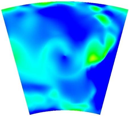
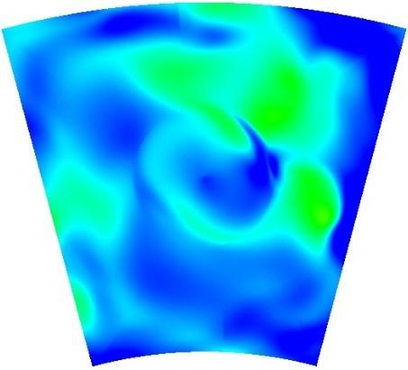
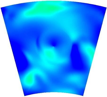
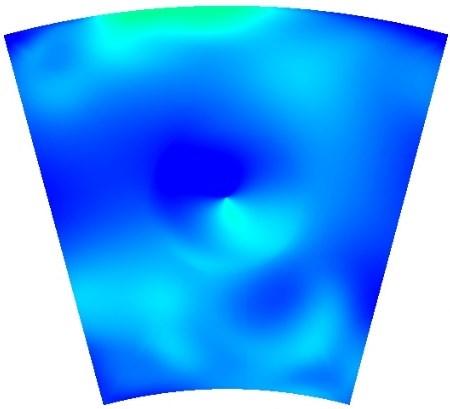
69 x/dh=0 x/dh=0.05 x/dh=0.1 x/dh=0.15 x/dh=0.2 x/dh=0.3 x/dh=0.4 x/dh=0.5 x/dh=1 Figure 44: Profiles of normalized tangential velocity at various X/Dh locations for Re = 50,000 59

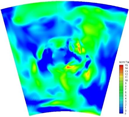
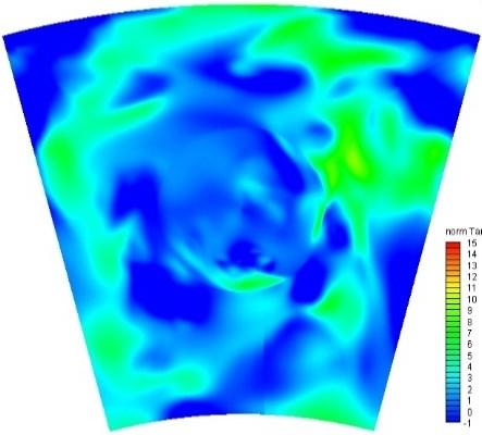
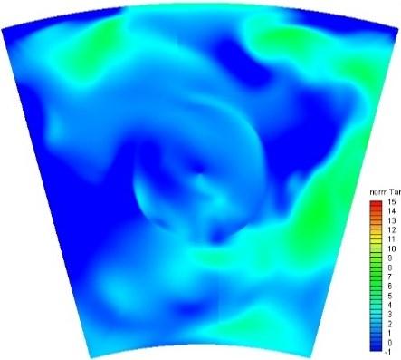
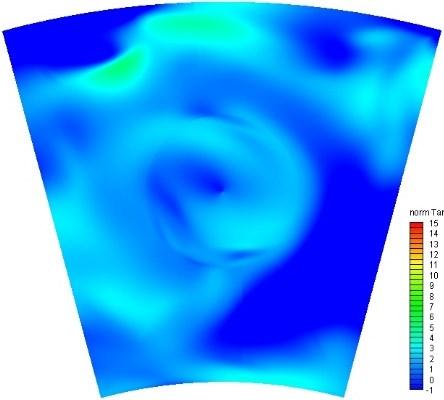
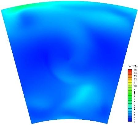
70 x/dh=0 x/dh=0.05 x/dh=0.1 x/dh=0.15 x/dh=0.2 x/dh=0.3 x/dh=0.4 x/dh=0.5 x/dh=1 Figure 45: Profiles of normalized tangential velocity at various X/Dh locations for Re = 840,000 60